Temporal patterns in daily measurements of inorganic and organic speciated PM_2.5 in Denver

Abstract

Airborne particulate matter less than 2.5 μm in aerodynamic diameter (PM_2.5) has been linked to a wide range of adverse health effects and as a result is currently regulated by the U.S. Environmental Protection Agency. PM_2.5 originates from a multitude of sources and has heterogeneous physical and chemical characteristics. These features complicate the link between PM_2.5 emission sources, ambient concentrations and health effects. The goal of the Denver Aerosol Sources and Health (DASH) study is to investigate associations between sources and health using daily measurements of speciated PM_2.5 in Denver.

The datxa set being collected for the DASH study will be the longest daily speciated PM_2.5 data set of its kind covering 5.5 years of daily inorganic and organic speciated measurements. As of 2008, 4.5 years of bulk measurements (mass, inorganic ions and total carbon) and 1.5 years of organic molecular marker measurements have been completed. Several techniques were used to reveal long-term and short-term temporal patterns in the bulk species and the organic molecular marker species. All species showed a strong annual periodicity, but their monthly and seasonal behavior varied substantially. Weekly periodicities appear in many compound classes with the most significant weekday/weekend effect observed for elemental carbon, cholestanes, hopanes, select polycyclic aromatic hydrocarbons (PAHs), heavy n-alkanoic acids and methoxyphenols. Many of the observed patterns can be explained by meteorology or anthropogenic activity patterns while others do not appear to have such obvious explanations. Similarities and differences in these findings compared to those reported from other cities are highlighted.

1. Introduction

Ambient particulate matter (PM) has been associated with a wide range of health effects (Pope and Dockery, 2006) and as a result is currently regulated as a criteria pollutant by the U.S. Environmental Protection Agency (U.S. EPA, 1997). PM is present in the atmosphere in a broad array of sizes and chemical compositions, with each particle potentially containing a multitude of inorganic and organic constituents. The highly complex nature of PM makes it a challenging pollutant to fully characterize. Furthermore, PM originates from many natural and anthropogenic sources and atmospheric formation processes, thus complicating the task of regulation. Recent advances in chemical characterization and source apportionment of PM are helping investigators to identify the major contributing sources. This, in turn, should provide regulators with the tools necessary to create more efficient control strategies. Source identification could also help in interpreting the observed links between PM and adverse health outcomes.

The Denver Aerosol Sources and Health (DASH) study was designed to investigate the link between sources of PM less than 2.5 μm in diameter (PM_2.5) and health effects (Vedal et al., 2009). The DASH study uses a series of detailed daily chemical speciation measurements along with advanced factor analysis techniques to identify sources of PM_2.5 in Denver. This approach requires measurement of marker species for major sources or source types over a long time period. The species list for the DASH study includes inorganic ions, total elemental and organic carbon and individual organic molecular markers. These species are scheduled to be quantified daily for a total of 5.5 years at the DASH receptor site in Denver.

Speciated measurements are difficult and labor intensive and, as a result, studies have typically been limited by the number of marker species measured, the study duration and the sampling frequency (e.g., every sixth day). Bae et al. (2004) and Sheesley et al. (2007) recently published results on speciated PM_2.5 measurements from the St. Louis Supersite campaign including daily measurements of bulk carbon and organic molecular markers, thus providing the first look at a complete annual time series of speciated organic measurements. Numerous investigators involved with the Pittsburgh Air Quality Study campaign have also recently published a long time series of similar PM_2.5 speciation measurements (Polidori et al., 2006; Robinson et al., 2006a,b,c; Wittig et al., 2004). The Pittsburgh measurements also covered an entire year, though they were limited to an every 6th day sampling frequency for the organic molecular marker species during the majority of the study period.

This paper includes spectral and temporal pattern analysis of the longest and most complete organic speciated daily data set to date. Daily measurements in Denver to support the DASH study commenced on July 1, 2002. Bulk speciation data including inorganic ions and total carbon are included for the first 4.5 years of the study (Dutton et al., 2009a). Detailed organic analysis for 71 unique molecular marker species are included for the first 1.5 years of the study (Dutton et al., 2009b). These data provide information on long-term and short-term variability in speciated PM_2.5. Numerous periodicities were detected in the time series for these species including several that have not been observed before in certain classes of compounds.

2. Methods

2.1. PM_2.5 speciation data

The receptor site for the DASH study was located on the rooftop of a two-story school building 5.3 km east of downtown Denver in a residential neighborhood removed from the direct influence of any major industrial or point sources (Vedal et al., 2009). Sample collection started on July 1, 2002 with daily 24-h (midnight to midnight) filter collection on both Teflon and quartz fiber filters for inorganic and organic PM_2.5 speciation, respectively. Quantification of bulk species including mass, inorganic ions by ion chromatography and total carbon by thermal optical transmission has been completed through December 31, 2006, resulting in 4.5 years of daily measurements (detailed methods are described in Dutton et al., 2009a). Quantification of organic molecular markers by gas chromatography–mass spectrometry (GC–MS) including alkanes, cycloalkanes, polycyclic aromatic hydrocarbons (PAHs), methyl substituted PAHs (methyl-PAHs), oxygenated PAHs (oxy-PAHs), steranes, alkanoic acids, sterols and methoxyphenols has been completed through December 31, 2003 for a total of 1.5 years of daily measurements (detailed methods are described in Dutton et al., 2009b). All species measurements have been blank corrected using weekly field blanks analyzed in parallel with the daily samples.

2.2. Supplemental data

Meteorological data were collected for the entire study period from a community monitoring station located 6.9 km west of the receptor site and operated by the Colorado Department of Public Health and Environment (CDPHE). Meteorological parameters included temperature, relative humidity, barometric pressure, scalar wind speed and vector wind direction. Twenty-four hour averages were derived from the hourly meteorological data to compare with the daily filter measurements.

Hourly traffic count data from multiple roadways in and around Denver were obtained from the Colorado Department of Transportation (CDOT). Missing observations in the traffic count data were replaced by the mean of available observations stratified by month, weekday, hour and traffic flow direction. Twenty-four hour totals were created from the traffic data by summing the hourly observations (including both directions of traffic flow) at each location. Only traffic monitoring stations with at least 300 days of observations were utilized. The available traffic data represented total counts only and was not stratified by vehicle weight or class. We used estimated truck percentages available for the same locations based on 2006 observations (CDOT, 2006) to make inferences on the relative impact of trucks and passenger vehicles at each traffic monitor. It is expected that the general traffic conditions did not change substantially over the 2002–2006 study period.

2.3. Spectral analysis

Spectral analysis on the time series for each PM constituent was performed to identify important periodicities in the data. The length and completeness (ranging from 80 to 99%, depending on constituent) of this data set allowed for detailed spectral analysis of speciated PM_2.5 components. However, traditional Fourier analysis requires a 100% complete data set. Since many of the missing observations were grouped together in time, replacing the missing values with the mean (or geometric mean, or median) of nearby observations was not deemed appropriate. We instead utilized the Lomb–Scargle method (Press and Rybicki, 1989; Press, 1992; Ruf, 1999; Van Dongen et al., 1997, 1999, 2001), an approach for spectral analysis of unevenly sampled data. Hies et al. (2000) compared spectral analyses on air pollution data containing missing observations using the Lomb–Scargle method with traditional Fourier analysis after zero-padding the data (i.e., replacing all missing observations with zero) and found similar results.

The Lomb–Scargle normalized periodogram (P) as a function of angular frequency (ω) is defined by:

$$\begin{array}{cc}\hfill P\left(\omega \right)=& \frac{1}{2{\sigma }^2}(\frac{{\left[\sum _{i=1}^n(x_i-\stackrel{‒}{x})\cos \left(\omega \right(t_i-\tau \left)\right)\right]}^2}{\sum _{i=1}^n{\cos }^2\left(\omega \right(t_i-\tau \left)\right)}\phantom{)}\hfill \\ \hfill & +\phantom{(}\frac{{\left[\sum _{i=1}^n(x_i-\stackrel{‒}{x})\sin \left(\omega \right(t_i-\tau \left)\right)\right]}^2}{\sum _{i=1}^n{\sin }^2\left(\omega \right(t_i-\tau \left)\right)})\hfill \end{array}$$ (1)

In Equation (1), x_i is the ith measurement (i = 1,…,n) observed at time t_i, $\stackrel{‒}{x}$ and σ are the mean and standard deviation of the measurements, and τ is an offset parameter defined by the relation:

$$\tan \left(2\omega \tau \right)=\frac{\sum _{i=1}^n\sin \left(2\omega t_i\right)}{\sum _{i=1}^n\cos \left(2\omega t_i\right)}$$ (2)

The inclusion of the offset parameter τ makes P(ω) unaffected by a constant time shift in the data (Press, 1992) and, furthermore, makes the periodogram equivalent to what one would obtain by fitting a series of harmonic functions to the data using linear least-squares regression (Lomb, 1976). This simplifies the interpretation of the Lomb–Scargle periodogram and explains why it is able to handle missing or unevenly sampled time series data.

Periodograms were generated for each of the species under investigation. The number of frequencies included in the spectrum was chosen to be two times the number of data points in the time series (Press, 1992). The individual peaks were smoothed using a Daniell smoothing kernel to reduce the variability in the spectrum (Bloomfield, 2000; Daniell, 1946). A triangular-shaped Daniell(1,1) weighting function (incorporating the five nearest frequencies) was chosen for smoothing the periodograms from the 1.5 year data sets and a similar Daniell(3,3) weighting function (incorporating the thirteen nearest frequencies) was chosen for smoothing the periodograms from the 4.5 year data sets. The selection of these two smoothing kernels resulted in approximately equal resolution in the frequency domain for the different length data sets.

Parametric methods exist for determining the statistical significance of the peaks present in the Lomb–Scargle periodograms (Press, 1992). These, however, rely on the assumption of normally distributed data (Schimmel, 2001). Rather than testing each time series to see if these criteria were met, and performing transformations if the criteria were not met, we chose instead to use a nonparametric bootstrap technique for determining significance (Efron, 1981, 1985). One thousand bootstrap samples were generated for each time series and the 95th percentile of the resulting smoothed periodograms was used to determine the 95% spectral significance level in a manner similar to Tourre et al. (2001). Furthermore, since environmental data frequently exhibit temporal autocorrelation (Piegorsch and Bailer, 2005) resulting in a low-frequency background in the spectrum, a 1-day lag autoregressive model [AR(1)] was fit to each time series and 1000 random simulations were generated using the optimum AR(1) model parameters. The 95th percentile of the simulated, smoothed periodograms was used to derive a second confidence bound indicating which peaks represent structure in the data above what would be expected from an AR(1) process. Peaks extending above both the bootstrap resample confidence bound and the AR(1) simulation confidence bound were considered to represent significant periodicities in the time series. The R statistical package (R Development Core Team, 2006) was used to perform the Lomb–Scargle spectral analysis, bootstrap significance and AR(1) simulations.

Suggested correspondence between the spectra for two different time series was achieved by pairing up significant spectral peaks or frequency bands. A more formal approach is commonly used in traditional Fourier analysis where coherence spectra are generated to identify more subtle temporal correlations between two time series at specific frequencies. For example, Hies et al. (2000) used coherence spectra to identify significant spectral relationships between EC and wind speed as well as EC and traffic counts. Our decision to use the Lomb–Scargle periodogram to avoid the need to impute missing values precluded the use of coherence spectra. This shortcoming was overcome by pairing the spectral results with temporal pattern analyses and weekday/weekend significance testing.

2.4. Temporal pattern analysis and significance testing

Box plots were used to visually test for hypothesized day of the week and seasonal patterns in the time series for each species. Exploratory investigation into other patterns was accomplished by stratifying the data by meteorological parameters such as temperature and wind speed. Wind rose plots generated using the 24-h averaged concentration data and the vector wind data proved to be misleading due to the complex and varying wind patterns in the area (Neff, 1997) and the lack of collocated meteorological data at the receptor site. Similar difficulties interpreting wind direction findings were encountered in Pittsburgh by Zhou et al. (2004); further discussion on the topic can be found in Watson et al. (2008). Wind direction was therefore omitted from further investigation. A two-sided, two-sample t-test (allowing for unequal variances) was used to test for differences between the mean concentration measured on weekdays (Mon–Fri) and weekends (Sat and Sun).

2.5. Compound classifications

A complete list of all 71 organic molecular marker species quantified in the daily samples is included in Dutton et al. (2009b). In an effort to reduce the number of individual results presented in this paper without losing any of the temporal information, certain groups of molecular marker compounds with similar chemical structures and temporal patterns were combined by summing their individual contributions. Nineteen n-alkanes ranging from C22 to C40 and seven n-alkanoic acids ranging from C12 to C18 were quantified. Fig. 1 shows the study – long average concentration for these aliphatic compounds ordered by carbon number. The n-alkanoic acids exhibit an even carbon preference while the lighter n-alkanes (C22–C34) exhibit an odd carbon preference similar to observations elsewhere (Hays et al., 2002; Schauer et al., 2001). After verifying similarity in their day of the week and seasonal patterns, the n-alkanes were summed into three groups: lighter even n-alkanes (C22–C34, even), lighter odd n-alkanes (C23–C33, odd) and heavier n-alkanes (C35–C40). The latter group did not exhibit any clear odd/even preference. Similarly, the n-alkanoic acids were summed into two groups: even n-alkanoic acids (C12–C18, even) and odd n-alkanoic acids (C13–C17, odd). Two cycloalkanes, pentadecylcyclohexane (C21) and nonadecylcyclohexane (C25), were quantified but showed slightly different patterns and therefore were not grouped together. The three cycloalkanes with mass to charge ratios (m/z) between these two were not quantified due to frequent coelution with the n-alkanes. Two unsaturated fatty acids (palmitoleic acid and oleic acid) were quantified, but did not have a sufficient number of detectable observations and therefore were omitted from the current analysis.

Fig. 1.

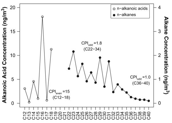
Average n-alkanoic acid and n-alkane concentrations by carbon number. The odd and even carbon preference indexes (CPI_odd and CPI_even) represent the ratio of odd-to-even and even-to-odd concentrations averaged over the range of carbon numbers shown in parenthesis.

The aromatic compounds quantified included 15 PAHs, 14 methyl-PAHs and 7 oxy-PAHs. All of the PAHs were highly correlated and showed similar day of the week and seasonal patterns. Because they cover such a broad range of molecular weights, however, they were summed into three groups by weight: lighter PAHs (fluoranthene–chrysene; m/z = 202–228), middle PAHs (benzo[b]fluoranthene–perylene; m/z = 252) and heavier PAHs (indeno[1,2,3cd]pyrene–coronene; m/z 276–300). The methyl-PAHs and oxy-PAHs did not show the same degree of within class correlation and were therefore broken down into groups based on their markedly different day of the week and temporal patterns: methyl-PAHs (m/z = 242 and 216, excluding retene), retene (m/z = 234), lighter oxy-PAHs (m/z = 168–180), middle oxy-PAHs (m/z = 196–208) and benz[de]anthracene-7-one (m/z = 230).

Three cholestanes and seven hopanes were quantified and all showed a high degree of within class correlation. They were summed into two groups: cholestanes and hopanes. Two sterols, cholesterol and stigmasterol, were quantified but left as separate entities as a result of differences in seasonal and day of the week patterns. Finally, five methoxyphenols were quantified including vanillin, acetovanillone, coniferaldehyde, syringaldehyde and acetosyringone (m/z = 152–196). These five compounds showed a high degree of correlation and remarkably similar temporal patterns and as a result were summed into one methoxyphenol group. The above compound groupings are supported by within class correlations observed in the data (Dutton et al., 2009b) and are generally consistent with available source profiles for organic molecular marker compounds (Cass, 1998; Schauer et al., 1996).

3. Results

3.1. Spectral analysis

Lomb–Scargle spectral analysis was performed on the meteorological data, traffic counts, individual species and the grouped species sums. With the exception of the traffic data, all showed significant spectral power at low frequency resulting from a combination of annual periodicities, linear trends, and low-frequency noise resulting from the finite length of the time series (Brittain et al., 2007; Hall et al., 2000). In general, the time series should be at least 10 times longer than the longest periodicity of interest (Wastler, 1963). Therefore, even the annual periodicity observed in the 4.5 years of bulk speciation data will be influenced by low-frequency artifacts. This, however, is not of concern since we know a priori that there are annual cycles in the data driven by meteorology and therefore spectral identification of the annual periodicity is not of particular interest. Aside from the low-frequency signal, only a few significant periodicities were present in the data; Fig. 2 shows a representative set of periodograms.

Fig. 2.

Lomb–Scargle periodograms for selected meteorological, traffic count, and pollutant time series data with significant spectral peaks identified by their respective period (T, in units of days). The significance bounds were generated using bootstrap techniques and AR(1) simulations as described in the text. The characters at the bottom of each plot identify the positioning of potential annual (a), monthly (m) and weekly (w) periods. In addition, the positioning of the first (w’) and second (w”) harmonics for the weekly period is depicted.

Of the meteorological parameters, temperature and barometric pressure revealed only the annual peak, but wind speed (Fig. 2a) and relative humidity (Fig. 2b) had significant peaks at multiple frequencies. The corresponding periods (T) range from 3.7 to 21.6 days for wind speed and 5.3–37.9 days for relative humidity. In several instances, the significant peaks were grouped together in close frequency bands (in such instances, only the most dominant period has been labeled in the figure). Of the speciated pollutants, only sulfate (Fig. 2c) had a large number of significant spectral peaks (or significant frequency bands) with corresponding periods of 4.0, 4.8, 6.3, 12.0 and 31.0 days. The three shortest periods match well with significant periods in the wind speed spectrum and the two longer periods match roughly with significant periods in the relative humidity spectrum. The sum of the middle oxy-PAHs (Fig. 2d) had a significant peak at 5.1 days.

Fig. 2e contains the periodogram for the traffic count data obtained from the nearest traffic monitor located on Colorado Blvd. at Colfax Ave., a heavily traveled surface street located 1.6 km northwest of the receptor site (median traffic count = 58,000 vehicles per day with an estimated truck percentage of 2.5% during weekday peak hours and 3.0% during weekday off-peak hours). This periodogram shows a clear weekly cycle with significant peaks at 7.0, 3.5 and 2.3 days. The shorter two periods (T = 3.5 and 2.3 days) are integer fractions of the weekly period (T = 7.0 days) and represent the first and second harmonics of the weekly period, respectively. The harmonics result from the non-sinusoidal shape of the traffic count time series. These three peaks are the only significant peaks between 0.0027 and 0.5 day⁻¹ (the Nyquist frequency for the 24-h counts) observed in the full year of traffic data. Therefore, any pollutant concentrations strongly linked to mobile sources are expected to have contributions at these frequencies (or at least one peak corresponding to the prominent seven day period).

Elemental carbon (EC, Fig. 2f) mimics the traffic data with a dominant 7-day period and two harmonics at 3.5 and 2.3 days. A significant weekly period (T = 7.0 days) was also present for the hopanes (Fig. 2g), steranes (not shown, but very similar to the hopanes), and the even n-alkanoic acids (Fig. 2h). The even n-alkanoic acids also contained a small significant peak at 4.0 days (the odd n-alkanoic acids did not contain any significant peaks). Closer inspection of the individual species periodograms revealed that the 4.0-day peak is being driven primarily by the heavier two even n-alkanoic acids (C16 and C18).

The remaining speciated compounds and compound groupings did not show significant peaks in the periodograms aside from the low-frequency background peak. These include nitrate, organic carbon (OC), alkanes, cycloalkanes, PAHs, methyl-PAHs, lighter and heavier oxy-PAHs, odd n-alkanoic acids, sterols and methoxyphenols.

3.2. Day of the week and seasonal patterns

Hypothesized patterns in the time series for PM_2.5 constituents included weekly cycles driven by anthropogenic day of the week emission patterns and annual cycles driven by meteorology. Other patterns could be present in the data reflecting, for instance, monthly or quarterly changes in industrial production, but these were expected to be small compared to any weekly or annual patterns. Box plots stratified by day of the week and month were used to visualize weekly and annual patterns in the data. Box plots for several of the bulk measurements and selected groups of organic molecular marker species are included in Figs. 3–5. Additional box plots for temperature, relative humidity, wind speed and traffic count data along with an expanded set of organic molecular marker species and PM_2.5 mass are provided in Figs. S1 through S7 in the Supplemental material.

Fig. 3.

Day of the week and seasonal box plots for a) nitrate, b) sulfate, c) OC and d) EC. The boxes depict the median (dark line), inner quartile range (shaded box), 10th and 90th percentiles (whiskers) and the mean (asterisk). The dashed line across the plot is the overall median. The individual median values and the number of points contained within each box are listed below the boxes.

Fig. 5.

Day of the week and seasonal box plots for a) middle PAHs, b) methyl-PAHs, c) benz[de]anthracene-7-one and d) hopanes. The boxes depict the median (dark line), inner quartile range (shaded box), 10th and 90th percentiles (whiskers) and the mean (asterisk). The dashed line across the plot is the overall median. The individual median values and the number of points contained within each box are listed below the boxes.

The day of the week box plots for the bulk species in the left-hand column of Fig. 3 confirm the lack of any significant weekly patterns in nitrate (Fig. 3a), sulfate (Fig. 3b) or OC (Fig. 3c). EC (Fig. 3d), on the other hand, shows a pronounced drop on Saturday followed by a second drop on Sunday. The total reduction in mean EC concentration from Friday to Sunday was 43%. This two-stage weekend decrease in EC is similar to that observed in the traffic count data (see Fig. S2 in the Supplemental material) where a 33% reduction in mean vehicle counts from Friday to Sunday was observed at the nearest traffic monitor.

The seasonal behavior of the bulk species is illustrated by the monthly box plots in the right-hand column of Fig. 3. This figure shows a typical reduction in nitrate (Fig. 3a) during the warmer summer months resulting from temperature-driven partitioning and volatilization, a rise in sulfate (Fig. 3b) and OC (Fig. 3c) during the summer resulting from increased photochemistry and/or emissions, and a gradual increase in EC (Fig. 3d) from April through December followed by a quick drop in January, February and March. Further discussion of the seasonal trends in the bulk species is contained in Dutton et al. (2009a).

As discussed earlier, the organic molecular marker species were pooled into groups based on compound class; box plots for all groupings are included in Figs. S3 through S6 in the Supplemental material. Fig. 4 contains box plots for selected groups of alkanes, alkanoic acids and methoxyphenols. There was no apparent day of the week pattern in any of the n-alkane groupings (lighter even and odd n-alkanes shown in Fig. 4a and b, respectively). The n-alkanoic acids (Fig. 4c) and methoxyphenols (Fig. 4d), however, show a slight weekend increase peaking on Saturday. A large summertime peak indicative of photochemistry or increased summertime emissions was observed in the odd n-alkanes (Fig. 4b) and even n-alkanoic acids (Fig. 4c). In contrast, the methoxyphenols (Fig. 4d) show a strong inverse correlation with temperature. The low readings for January (relative to December and February) reflect a January temperature anomaly where the median temperature integrated over the study period was 2 °C warmer in January than neighboring months (see Fig. S1 in the Supplemental material).

Fig. 4.

Day of the week and seasonal box plots for a) lighter even n-alkanes, b) lighter odd n-alkanes, c) even n-alkanoic acids and d) methoxyphenols. The boxes depict the median (dark line), inner quartile range (shaded box), 10th and 90th percentiles (whiskers) and the mean (asterisk). The dashed line across the plot is the overall median. The individual median values and the number of points contained within each box are listed below the boxes.

The PAHs (middle weight PAHs shown in Fig. 5a), methyl-PAHs (Fig. 5b), benz[de]anthracene-7-one (Fig. 5c) and hopanes (Fig. 5d) all had the lowest median values on the weekends, specifically Sunday. The reduction in daily mean from Friday to Sunday was 28%, 32%, 26% and 35% for the middle PAHs, methyl-PAHs, benz[de]anthracene-7-one and the hopanes, respectively. The seasonal patterns for the PAHs, methyl-PAHs and benz[de]anthracene-7-one are similar and appear to be dominated by meteorology with maximum readings in December consistent with both temperature-driven partitioning and dilution effects. This is further supported by a slight decrease in these species in January relative to neighboring months reflecting the January temperature anomaly. The hopanes also peak in December, but have less seasonal dependence.

3.3. Weekday verses weekend significance test

Many species showed a statistically significant difference between the mean recorded on weekdays (Monday–Friday) versus weekends (Saturday and Sunday). Table 1 lists all the species with a statistically significant difference at the 95% confidence level; the table is sorted by the percent reduction on weekends. EC had the largest percent decrease on weekends (−33%; 95% confidence = −27 to −38%; p-value < 0.0001). Syringaldehyde had the largest percent increase on weekends (52%; 95% confidence interval = 9–95%; p-value = 0.0189).

Table 1.

Species with statistically significant weekday/weekend mean differences.

Species	Weekday meana	Weekend meana	Percent changeb	Lower 95% CIc	Upper 95% CIc	P-valuec
EC	0.61	0.41	−33	−38	−27	<0.0001
22s-ab-30-Homohopane	0.10	0.07	−28	−40	−17	<0.0001
Benzo[ghi]fluoranthene	0.10	0.08	−28	−43	−12	0.0006
ba-30-Norhopane	0.38	0.28	−27	−38	−16	<0.0001
ab-Hopane	0.24	0.17	−27	−39	−16	<0.0001
22r-ab-30-Bishomohopane	0.05	0.04	−26	−38	−15	<0.0001
20r-abb & 20s-aaa-Cholestane	0.15	0.12	−25	−34	−16	<0.0001
a-22,29,30-Trisnorhopane	0.09	0.07	−25	−34	−16	<0.0001
22s-ab-30-Bishomohopane	0.06	0.05	−25	−37	−12	0.0002
Pyrene	0.17	0.13	−25	−42	−7	0.0054
20r & s-abb-Ethylcholestane	0.12	0.09	−24	−34	−14	<0.0001
Methyl-202-pah sum	0.66	0.50	−24	−42	−7	0.0068
20r & s-abb-Methylcholestane	0.11	0.08	−23	−35	−11	0.0003
22r-ab-30-Homohopane	0.07	0.06	−23	−37	−9	0.0013
Benz[a]anthracene	0.06	0.05	−23	−44	−3	0.0244
Chrysene/triphenylene	0.18	0.14	−21	−35	−6	0.0053
Coronene	0.11	0.08	−21	−37	−4	0.0146
1,8-Naphthalic anhydride	0.33	0.26	−20	−30	−11	<0.0001
Benzo[ghi]perylene	0.22	0.18	−19	−37	−1	0.0396
Fluoranthene	0.20	0.17	−18	−34	−3	0.0175
Methyl-228-pah sum	0.12	0.10	−17	−33	−2	0.0263
TC	3.69	3.44	−7	−11	−2	0.0026
Hexadecanoic acid	16.95	20.91	23	6	41	0.0102
Nonatriacontane	0.14	0.18	29	3	56	0.0300
Octadecanoic acid	10.43	13.41	29	7	50	0.0091
Heptadecanoic acid	0.56	0.77	36	13	58	0.0019
Acetovanillone	0.52	0.72	39	6	72	0.0219
Coniferaldehyde	1.07	1.56	46	4	87	0.0305
Syringaldehyde	1.05	1.59	52	9	95	0.0189

^aEC and TC are in μg m⁻³; all other species are in ng m⁻³.

^bPercent change from the weekday mean to the weekend mean (negative values indicate a weekend decrease; positive values indicate a weekend increase.

^cResults froma two-sided t-test comparing weekday mean toweekend mean allowing for unequal variances (only species showing a significant difference at the 95% confidence level are included and are sorted by the percent change). The upper and lower 95% confidence intervals (CI) are displayed as a percent change from the weekday mean.

4. Discussion

4.1. Spectral signatures

The Lomb–Scargle periodograms proved to be a useful tool for identifying significant periodicities in the time series data without the need to fill in missing observations or form prior hypotheses on anticipated patterns. Significant spectral peaks in the sulfate data shown in Fig. 2c coincided with those in the wind speed (Fig. 2a) and relative humidity (Fig. 2b) periodograms, suggesting that sulfate concentrations are directly influenced by meteorology. Sulfate demonstrated a small negative correlation with wind speed (R = −0.21) and slightly larger positive correlation with relative humidity (R = 0.40). Higher winds are expected to enhance mixing and therefore potentially reduce sulfate concentrations. Ammonium sulfate formation is also dependent on the aqueous content of the aerosol and therefore is expected to increase with humidity (Tursic et al., 2003). Sulfate was the only species to show multiple significant spectral peaks. The sum of the middle oxy-PAHs shown in Fig. 2d had a significant peak at 5.1 days which corresponds roughly with spectral bands in the wind speed and relative humidity periodograms. However, since none of the other significant meteorological peaks appear as significant peaks in the middle oxy-PAH spectrum, this species does not show as clear a correspondence with meteorology as sulfate does. No obvious anthropogenic emission patterns occur with a frequency of 5.1 days, so the significant spectral peak in the middle oxy-PAH spectrum is currently unexplained.

EC in Fig. 2f showed the most striking periodogram, mimicking the three peaks in the traffic count periodogram (Fig. 2e). The hopanes (Fig. 2g) and even n-alkanoic acids (Fig. 2h) also had significant spectral signatures with a weekly periodicity, suggestive of an anthropogenic source. Both EC and hopanes are indicative of motor vehicle emissions (Cadle et al., 1999; Fraser et al., 2002; Lough et al., 2007; Rogge et al., 1993a; Schauer et al., 1999b, 2002b) and therefore their spectral signatures are in agreement with the traffic count spectra resulting from a pronounced decrease in motor vehicle traffic on the weekends.

Several compounds which were expected to show significant weekly periodicity did not stand out in the Lomb–Scargle periodograms. For example, PAHs – which are also prominent in motor vehicle emissions – were expected to have a significant peak at seven days corresponding to weekly traffic patterns. Investigation using box plots and weekday/weekend significance tests confirmed the expected weekly patterns. Measurement uncertainty, contributions from other uncorrelated sources and a strong seasonal fluctuation in concentrations may have prevented any significant weekly pattern from showing up in the spectral signature for the PAHs. It is possible that these periodicities will stand out above the noise when a longer time series is analyzed.

4.2. Seasonal variability

The seasonal box plots were useful in illustrating the shape of the seasonal patterns for each constituent. Many species had a summertime peak centered on July and August, the warmest two months of the year. The most pronounced summertime peaks were observed in total OC (Fig. 3c), lighter odd n-alkanes (Fig. 4b), n-alkanoic acids (Figs. 4c and S6b) and middle oxy-PAHs (Fig. S5b). The substantial summertime peak in total OC is too large to be explained by increases in the molecular marker species alone and likely contains additional contributions from enhanced summertime emissions or photochemical processing of uncharacterized organic compounds. The lighter odd n-alkanes and n-alkanoic acids are present in leaf abrasion products (Cass, 1998; Rogge et al., 1993b) and plant waxes (Simoneit and Mazurek, 1982), making these peaks consistent with increased leaf abrasion emissions during the growing season. If the source of these emissions was purely leaf abrasion, however, the peak would likely persist into the fall. The clear summertime peak centered in July indicates that these species are probably coming from more complex biogenic emission processes in addition to simple leaf abrasion.

A slight anomaly in the sinusoidal pattern in temperature observed during January (Fig. S1a) was helpful in identifying species with strong temperature dependence. They include nitrate, PAHs, methyl-PAHs, oxy-PAHs and methoxyphenol. All of these species were anti-correlated with temperature and therefore show a resulting decrease in January relative to December and February. This dependence could be driven by formation kinetics, gas-particle partitioning, and/or emissions behavior. Methoxyphenols are likely influenced at least in part by emissions behavior since they are prominent in wood smoke (Cass, 1998; Chow et al., 2007; Schauer et al., 2001; Simoneit et al., 1993) and the residential use of fireplaces is directly linked with ambient temperature.

4.3. Day of the week observations

A weekly cycle was expected in constituents with emissions dominated by mobile sources, biomass combustion and meat cooking based on source activity patterns reported by Chinkin et al. (2003). Motor vehicle traffic counts included in Fig. S2 in the Supplemental material show a gradual build-up during the work-week and a two-stage drop off on the weekends. This same pattern has been observed in urban areas in Atlanta (Cardelino, 1998), Southern California (Chinkin et al., 2003) and the San Francisco Bay Area (Harley et al., 2005; Marr et al., 2002). Traffic data shown in Fig. S2e for a major highway connecting Denver with other cities further north (monitor located 30 km from the receptor site) show higher relative traffic counts on Friday, Saturday and Sunday compared with the other traffic monitors included in Fig. S2. This is consistent with motorists traveling to or from Denver for weekend activities and was also observed at rural monitoring stations outside Atlanta and San Francisco in the studies cited above. Given the consistency in weekday traffic patterns on the in-town streets and the greater distance to the differing traffic patterns located out-of-town, we expect the influence of motor vehicle emissions on our receptor site to reflect the patterns observed at the nearby streets.

In studies where traffic data stratified by vehicle class has been available, investigators have observed a much smaller percentage decrease in passenger vehicle traffic on weekends relative to truck traffic. Chinkin et al. (2003) reported a 20% decrease in passenger vehicles from Friday to Sunday and a corresponding 67% decrease in heavy-duty trucks. Marr et al. (2002) reported 16% and 82% decreases, respectively. Unfortunately, we did not have access to traffic data stratified by vehicle class. However, we do have an estimate of the average weekday truck percentage at each traffic monitoring site during peak (i.e., rush hour) and off-peak hours. We used these truck percentages to derive an estimated range for the percent decrease in passenger vehicles from Friday to Sunday at each traffic monitoring location. This was done by varying the range of possible truck traffic reductions from 0 to 100% on the weekends and estimating the additional decrease in passenger vehicle reductions required to match the overall traffic counts. The estimated decrease in mean passenger vehicle counts from Friday to Sunday at the nearest traffic monitor was 31–34%. The remaining nearby sites gave similar estimates for this range while the out-of-town monitor located 30.3 km north had a lower range of 0–17%. These are only rough estimates, but they suggest a slightly larger weekend reduction in passenger vehicle traffic on the nearby streets in Denver than has been observed in the other cities mentioned above. Therefore, any observed weekend effect in mobile source pollutants is not necessarily a result of reductions in the diesel fleet alone since passenger vehicle miles driven drop appreciably on the weekends as well. Reductions in other industrial emissions on weekends due to scaled back or suspended production could also be responsible for some of the observed weekend decrease in pollutant concentrations.

EC had the largest weekend decrease (relative to weekdays; see Table 1) with concentrations dropping 43% on average from Friday to Sunday. This is appreciably larger than the corresponding 33% reduction in overall traffic counts at the closest traffic monitor or the 31–34% estimated reduction from passenger vehicle traffic counts alone. This confirms the importance of diesel vehicles in explaining the large and significant EC weekend effect and is consistent with EC being a major constituent of diesel emissions (Diaz-Robles et al., 2008). Similar weekend decreases in EC have been observed at various locations in California (Lough et al., 2006; Motallebi et al., 2003), St. Louis (Bae et al., 2004; Sheesley et al., 2007) and Pittsburgh (Allen et al., 1999). Our observed 43% reduction in EC from Friday to Sunday lies between a 30% reduction reported by Bae et al. (2004) for EC in St. Louis and a 54% reduction reported by Allen et al. (1999) for black carbon in Pittsburgh. It is substantially less than the 73% and 76% reductions observed by Lough et al. (2006) for EC in Los Angeles and Azusa, respectively. These latter two sites were heavily impacted by industry and motor vehicle traffic, particularly Azusa which had a high prevalence of heavy-duty diesel truck traffic. Measurements at the Pittsburgh and California sites took place in the summertime over an eleven and three-week study period, respectively, and it is not clear if the larger weekend effects would persist on an annual basis.

Twenty molecular marker species in addition to EC and TC showed a significant decrease on weekends. These included all of the steranes, many of the PAHs and some of the methyl-PAHs and oxy-PAHs (see Table 1). Although the percent reduction observed in the molecular markers were not as large as EC, they were still highly significant in many instances, particularly for the steranes (a marker for motor oil combustion; Schauer et al., 1996; Rogge et al., 1993a). Lough et al. (2006) found a similar reduction on the weekends (specifically Sunday) over a three-week measurement period in Los Angeles for the same suite of steranes measured here. Sheesley et al. (2007), however, did not find any weekend drop in two quantified hopanes in St. Louis despite seeing a substantial drop in EC. The St. Louis study covered a full year of samples, so this discrepancy is not the result of short-term variability. Consistency between Denver and St. Louis in the weekend effect for EC but not the hopanes may be the result of differing gasoline and diesel motor vehicle usage patterns influencing the receptor sites for these two cities. It is plausible that the weekend reduction in passenger vehicle use is more pronounced in Denver than St. Louis, resulting in the observed significant decrease in steranes and PAHs in addition to EC. It is also possible that an increase in non-road combustion engine emissions (e.g., lawnmowers) counteracted any reductions in on-road vehicle emissions on weekends in St. Louis. This also helps explain the smaller percent decrease in steranes relative to EC on weekends in Denver and Los Angeles.

Significant weekend increases were observed in seven organic molecular marker species including three methoxyphenols, three heavier n-alkanoic acids and one heavy n-alkane (see Table 1). All of the methoxyphenols and the heavier n-alkanoic acids peaked on Saturday while nonatriacontane peaked on Sunday. Methoxyphenols are frequently used as markers for wood combustion (Chow et al., 2007; Schauer et al., 2001). Survey results on weekly patterns in residential fireplace use reported by Chinkin et al. (2003) show a peak on Saturday followed next by Friday and Sunday. This is consistent with day of the week patterns observed in the methoxyphenols (Fig. 4d). Therefore, the observed weekend increase in this class of compounds is likely a result of increased weekend fireplace use in Denver. Similar weekend increases in syringaldehyde (one of the six methoxyphenols we quantified) were observed by Robinson et al. (2006b) in Pittsburgh. Lough et al. (2006) found elevated concentrations of levoglucosan (another wood smoke marker not quantified in our study) on Thursday, Friday and Saturday in Los Angeles and Azusa.

The peak in the n-alkanoic acids was driven by the heavier compounds (C15–C18) which showed a similar day of the week pattern to the methoxyphenols, peaking on Saturday with Sunday also elevated relative to the rest of the week. The even n-alkanoic acids were one of the few compound classes that also showed significant spectral significance at a period of seven days (Fig. 2h). These aliphatic acids, particularly hexadecanoic acid, are present in wood smoke from combustion of various types of wood (Fine et al., 2001, 2002, 2004; Rogge et al., 1998; Schauer et al., 2001). However, they are also prevalent in meat cooking and seed oil cooking emissions, particularly hexadecanoic acid and octadecanoic acid (Schauer et al.,1999a, 2002a). Barbecuing is another emission source expected to increase on weekends based on survey results (Chinkin et al., 2003) with elevated contributions on both Saturday and Sunday. It is also reasonable to expect an increase in restaurant patronage on weekends relative to weekdays. Therefore, the significant increase in the heavier n-alkanoic acids on weekends is consistent with both fireplace use and food cooking activity patterns. Cholesterol and oleic acid are two molecular markers commonly associated with meat cooking (Cass, 1998; Rogge et al., 1991). As mentioned earlier, oleic acid was quantified but did not have a sufficient number of detectable observations to be considered in the current analysis. Cholesterol also suffered from a large number of observations below detection limit (73% of all observations) as a result of high field blank contamination. The signal to noise ratio (mean concentration/mean uncertainty) for cholesterol was only 1.1 compared to 2.3–5.5 for the heavy n-alkanoic acids (Dutton et al., 2009b). This could explain the lack of weekly patterns observed in the spectral analysis, box plots and t-test for cholesterol despite the presence of a potential weekend increase in meat cooking.

5. Conclusions

The various short- and long-term patterns observed in this data set have shown suggestive correspondence with a variety of anthropogenic and natural emission source patterns. While the Lomb–Scargle analysis missed several organic molecular marker periodicities apparent in the box plots and confirmed by the weekday/weekend t-tests, it is expected that these different methods for pattern analysis will come into better agreement as the data set becomes more complete. At 1.5 years in length, however, it has already provided insight into temporal patterns not previously documented. The next step in identifying source contributions on a daily basis in Denver will involve formal factor analysis. The pattern analysis techniques demonstrated in this work will be helpful in making the link between the resulting factors and tangible PM_2.5 emission sources.

References

- Allen GA, Lawrence J, Koutrakis P. Field validation of a semi-continuous method for aerosol black carbon (aethalometer) and temporal patterns of summertime hourly black carbon measurements in southwestern PA. Atmospheric Environment. 1999;33:817–823. [Google Scholar]
- Bae MS, Schauer JJ, DeMinter JT, Turner JR. Hourly and daily patterns of particle-phase organic and elemental carbon concentrations in the urban atmosphere. Journal of the Air & Waste Management Association. 2004;54:823–833. doi: 10.1080/10473289.2004.10470957. [DOI] [PubMed] [Google Scholar]
- Bloomfield P. Fourier Analysis of Time Series: an Introduction. Wiley; New York: 2000. [Google Scholar]
- Brittain JS, Halliday DM, Conway BA, Nielsen JB. Single-trial multi-wavelet coherence in application to neurophysiological time series. IEEE Transactions on Biomedical Engineering. 2007;54:854–862. doi: 10.1109/TBME.2006.889185. [DOI] [PubMed] [Google Scholar]
- Cadle SH, Mulawa PA, Hunsanger EC, Nelson K, Ragazzi RA, Barrett R, Gallagher GL, Lawson DR, Knapp KT, Snow R. Composition of light-duty motor vehicle exhaust particulate matter in the Denver, Colorado area. Environmental Science & Technology. 1999;33:2328–2339. doi: 10.1080/10473289.1999.10463872. [DOI] [PubMed] [Google Scholar]
- Cardelino C. Daily variability of motor vehicle emissions derived from traffic counter data. Journal of the Air & Waste Management Association. 1998;48:637–645. doi: 10.1080/10473289.1998.10463709. [DOI] [PubMed] [Google Scholar]
- Cass GR. Organic molecular tracers for particulate air pollution sources. Trac-Trends in Analytical Chemistry. 1998;17:356–366. [Google Scholar]
- CDOT Straight Line Diagram Tool. Colorado Department of Transportation. 2006 http://dtdexternal.dot.state.co.us/sld/
- Chinkin LR, Coe DL, Funk TH, Hafner HR, Roberts PT, Ryan PA, Lawson DR. Weekday versus weekend activity patterns for ozone precursor emissions in California’s South Coast Air Basin. Journal of the Air & Waste Management Association. 2003;53:829–843. doi: 10.1080/10473289.2003.10466223. [DOI] [PubMed] [Google Scholar]
- Chow JC, Watson JG, Lowenthal DH, Chen LWA, Zielinska B, Mazzoleni LR, Magliano KL. Evaluation of organic markers for chemical mass balance source apportionment at the Fresno Supersite. Atmospheric Chemistry and Physics. 2007;7:1741–1754. [Google Scholar]
- Daniell PJ. Discussion on symposium on autocorrelation in time series. Journal of the Royal Statistical Society. 1946;8:88–90. [Google Scholar]
- Diaz-Robles LA, Fu JS, Reed GD. Modeling and source apportionment of diesel particulate matter. Environment International. 2008;34:1–11. doi: 10.1016/j.envint.2007.06.002. [DOI] [PubMed] [Google Scholar]
- Dutton SJ, Schauer JJ, Vedal S, Hannigan MP. PM2.5 characterization for time series studies: pointwise uncertainty estimation and bulk speciation methods applied in Denver. Atmospheric Environment. 2009a;43:1136–1146. doi: 10.1016/j.atmosenv.2008.10.003. [DOI] [PMC free article] [PubMed] [Google Scholar]
- Dutton SJ, Williams DE, Garcia JK, Vedal S, Hannigan MP. PM2.5 characterization for time series studies: organic molecular marker speciation methods and observations from daily measurements in Denver. Atmospheric Environment. 2009b;43:2018–2030. doi: 10.1016/j.atmosenv.2009.01.003. [DOI] [PMC free article] [PubMed] [Google Scholar]
- Efron B. Nonparametric estimates of standard error – the jackknife, the bootstrap and other methods. Biometrika. 1981;68:589–599. [Google Scholar]
- Efron B. Bootstrap confidence-intervals for a class of parametric problems. Biometrika. 1985;72:45–58. [Google Scholar]
- Fine PM, Cass GR, Simoneit BRT. Chemical characterization of fine particle emissions from fireplace combustion of woods grown in the north-eastern United States. Environmental Science & Technology. 2001;35:2665–2675. doi: 10.1021/es001466k. [DOI] [PubMed] [Google Scholar]
- Fine PM, Cass GR, Simoneit BRT. Chemical characterization of fine particle emissions from the fireplace combustion of woods grown in the southern United States. Environmental Science & Technology. 2002;36:1442–1451. doi: 10.1021/es0108988. [DOI] [PubMed] [Google Scholar]
- Fine PM, Cass GR, Simoneit BRT. Chemical characterization of fine particle emissions from the fireplace combustion of wood types grown in the Midwestern and Western United States. Environmental Engineering Science. 2004;21:387–409. [Google Scholar]
- Fraser MP, Lakshmanan K, Fritz SG, Ubanwa B. Variation in composition of fine particulate emissions from heavy-duty diesel vehicles. Journal of Geophysical Research-Atmospheres. 2002;107:8346. [Google Scholar]
- Hall P, Reimann J, Rice J. Nonparametric estimation of a periodic function. Biometrika. 2000;87:545–557. [Google Scholar]
- Harley RA, Marr LC, Lehner JK, Giddings SN. Changes in motor vehicle emissions on diurnal to decadal time scales and effects on atmospheric composition. Environmental Science & Technology. 2005;39:5356–5362. doi: 10.1021/es048172+. [DOI] [PubMed] [Google Scholar]
- Hays MD, Geron CD, Linna KJ, Smith ND, Schauer JJ. Speciation of gas-phase and fine particle emissions from burning of foliar fuels. Environmental Science & Technology. 2002;36:2281–2295. doi: 10.1021/es0111683. [DOI] [PubMed] [Google Scholar]
- Hies T, Treffeisen R, Sebald L, Reimer E. Spectral analysis of air pollutants. Part 1. Elemental carbon time series. Atmospheric Environment. 2000;34:3495–3502. [Google Scholar]
- Lomb NR. Least-squares frequency-analysis of unequally spaced data. Astrophysics and Space Science. 1976;39:447–462. [Google Scholar]
- Lough GC, Christensen CG, Schauer JJ, Tortorelli J, Mani E, Lawson DR, Clark NN, Gabele PA. Development of molecular marker source profiles for emissions from on-road gasoline and diesel vehicle fleets. Journal of the Air & Waste Management Association. 2007;57:1190–1199. doi: 10.3155/1047-3289.57.10.1190. [DOI] [PubMed] [Google Scholar]
- Lough GC, Schauer JJ, Lawson DR. Day-of-week trends in carbonaceous aerosol composition in the urban atmosphere. Atmospheric Environment. 2006;40:4137–4149. [Google Scholar]
- Marr LC, Black DR, Harley RA. Formation of photochemical air pollution in central California – 1. Development of a revised motor vehicle emission inventory. Journal of Geophysical Research-Atmospheres. 2002;107:1–9. [Google Scholar]
- Motallebi N, Tran H, Croes BE, Larsen LC. Day-of-week patterns of particulate matter and its chemical components at selected sites in California. Journal of the Air & Waste Management Association. 2003;53:876–888. doi: 10.1080/10473289.2003.10466229. [DOI] [PubMed] [Google Scholar]
- Neff WD. The Denver Brown Cloud studies from the perspective of model assessment needs and the role of meteorology. Journal of the Air & Waste Management Association. 1997;47:269–285. doi: 10.1080/10473289.1997.10464447. [DOI] [PubMed] [Google Scholar]
- Piegorsch WW, Bailer AJ. Analyzing Environmental Data. John Wiley, Chichester, West Sussex, England; Hoboken, NJ: 2005. [Google Scholar]
- Polidori A, Turpin BJ, Lim HJ, Cabada JC, Subramanian R, Pandis SN, Robinson AL. Local and regional secondary organic aerosol: insights from a year of semi-continuous carbon measurements at Pittsburgh. Aerosol Science and Technology. 2006;40:861–872. [Google Scholar]
- Pope CA, Dockery DW. Health effect of fine particulate air pollution: lines that connect. Journal of the Air & Waste Management Association. 2006;56:709–742. doi: 10.1080/10473289.2006.10464485. [DOI] [PubMed] [Google Scholar]
- Press WH. Numerical Recipes in C: the Art of Scientific Computing. Cambridge University Press; Cambridge, New York: 1992. [Google Scholar]
- Press WH, Rybicki GB. Fast algorithm for spectral-analysis of unevenly sampled data. Astrophysical Journal. 1989;338:277–280. [Google Scholar]
- R Development Core Team . R: a Language and Environment for Statistical Computing. R Development Core Team, R Foundation for Statistical Computing; Vienna, Austria: 2006. ISBN 3-900051-07-0. http://www.R-project.org. [Google Scholar]
- Robinson AL, Subramanian R, Donahue NM, Bernardo-Bricker A, Rogge WF. Source apportionment of molecular markers and organic aerosol. 1. Polycyclic aromatic hydrocarbons and methodology for data visualization. Environmental Science & Technology. 2006a;40:7803–7810. doi: 10.1021/es0510414. [DOI] [PubMed] [Google Scholar]
- Robinson AL, Subramanian R, Donahue NM, Bernardo-Bricker A, Rogge WF. Source apportionment of molecular markers and organic aerosol. 2. Biomass smoke. Environmental Science & Technology. 2006b;40:7811–7819. doi: 10.1021/es060782h. [DOI] [PubMed] [Google Scholar]
- Robinson AL, Subramanian R, Donahue NM, Bernardo-Bricker A, Rogge WF. Source apportionment of molecular markers and organic aerosol. 3. Food cooking emissions. Environmental Science & Technology. 2006c;40:7820–7827. doi: 10.1021/es060781p. [DOI] [PubMed] [Google Scholar]
- Rogge WF, Hildemann LM, Mazurek MA, Cass GR, Simoneit BRT. Sources of fine organic aerosol. 2. Noncatalyst and catalyst-equipped automobiles and heavy-duty diesel trucks. Environmental Science & Technology. 1993a;27:636–651. [Google Scholar]
- Rogge WF, Hildemann LM, Mazurek MA, Cass GR, Simoneit BRT. Sources of fine organic aerosol. 4. Particulate abrasion products from leaf surfaces of urban plants. Environmental Science & Technology. 1993b;27:2700–2711. [Google Scholar]
- Rogge WF, Hildemann LM, Mazurek MA, Cass GR, Simoneit BRT. Sources of fine organic aerosol. 9. Pine, oak and synthetic log combustion in residential fireplaces. Environmental Science & Technology. 1998;32:13–22. [Google Scholar]
- Rogge WF, Hildemann LM, Mazurek MA, Cass GR, Simonelt BRT. Sources of fine organic aerosol. 1. Charbroilers and meat cooking operations. Environmental Science & Technology. 1991;25:1112–1125. doi: 10.1021/es00056a030. [DOI] [PubMed] [Google Scholar]
- Ruf T. The Lomb–Scargle periodogram in biological rhythm research: analysis of incomplete and unequally spaced time-series. Biological Rhythm Research. 1999;30:178–201. [Google Scholar]
- Schauer JJ, Kleeman MJ, Cass GR, Simoneit BRT. Measurement of emissions from air pollution sources. 1. C-1 through C-29 organic compounds from meat charbroiling. Environmental Science & Technology. 1999a;33:1566–1577. [Google Scholar]
- Schauer JJ, Kleeman MJ, Cass GR, Simoneit BRT. Measurement of emissions from air pollution sources. 2. C-1 through C-30 organic compounds from medium duty diesel trucks. Environmental Science & Technology. 1999b;33:1578–1587. [Google Scholar]
- Schauer JJ, Kleeman MJ, Cass GR, Simoneit BRT. Measurement of emissions from air pollution sources. 3. C-1–C-29 organic compounds from fireplace combustion of wood. Environmental Science & Technology. 2001;35:1716–1728. doi: 10.1021/es001331e. [DOI] [PubMed] [Google Scholar]
- Schauer JJ, Kleeman MJ, Cass GR, Simoneit BRT. Measurement of emissions from air pollution sources. 4. C-1–C-27 organic compounds from cooking with seed oils. Environmental Science & Technology. 2002a;36:567–575. doi: 10.1021/es002053m. [DOI] [PubMed] [Google Scholar]
- Schauer JJ, Kleeman MJ, Cass GR, Simoneit BRT. Measurement of emissions from air pollution sources. 5. C-1–C-32 organic compounds from gasoline-powered motor vehicles. Environmental Science & Technology. 2002b;36:1169–1180. doi: 10.1021/es0108077. [DOI] [PubMed] [Google Scholar]
- Schauer JJ, Rogge WF, Hildemann LM, Mazurek MA, Cass GR. Source apportionment of airborne particulate matter using organic compounds as tracers. Atmospheric Environment. 1996;30:3837–3855. [Google Scholar]
- Schimmel M. Emphasizing difficulties in the detection of rhythms with Lomb–Scargle periodograms. Biological Rhythm Research. 2001;32:341–345. doi: 10.1076/brhm.32.3.341.1340. [DOI] [PubMed] [Google Scholar]
- Sheesley RJ, Schauer JJ, Meiritz M, DeMinter JT, Bae MS, Turner JR. Daily variation in particle-phase source tracers in an urban atmosphere. Aerosol Science and Technology. 2007;41:981–993. [Google Scholar]
- Simoneit BRT, Mazurek MA. Organic-matter of the troposphere. 2. Natural background of biogenic lipid matter in aerosols over the rural western United States. Atmospheric Environment. 1982;16:2139–2159. [Google Scholar]
- Simoneit BRT, Rogge WF, Mazurek MA, Standley LJ, Hildemann LM, Cass GR. Lignin pyrolysis products, lignans, and resin acids as specific tracers of plant classes in emissions from biomass combustion. Environmental Science & Technology. 1993;27:2533–2541. [Google Scholar]
- Tourre YM, Rajagopalan B, Kushnir Y, Barlow M, White WB. Patterns of coherent decadal and interdecadal climate signals in the Pacific Basin during the 20th century. Geophysical Research Letters. 2001;28:2069–2072. [Google Scholar]
- Tursic J, Berner A, Veber M, Bizjak M, Podkrajsek B, Grgic I. Sulfate formation on synthetic deposits under haze conditions. Atmospheric Environment. 2003;37:3509–3516. [Google Scholar]
- U.S. EPA . 40 CFR Part 50, 1997 Edition: National Primary and Secondary Ambient Air Quality Standards. Code of Federal Regulations. Environmental Protection Agency; Washington, DC: 1997. pp. 5–84. [Google Scholar]
- Van Dongen HPA, Olofsen E, VanHartevelt JH, Kruyt EW. Technical Report. Leiden University; The Netherlands: 1997. Periodogram Analysis of Unequally Spaced Data: the Lomb Method. [Google Scholar]
- Van Dongen HPA, Olofsen E, VanHartevelt JH, Kruyt EW. A procedure of multiple period searching in unequally spaced time-series with the Lomb–Scargle method. Biological Rhythm Research. 1999;30:149–177. doi: 10.1076/brhm.30.2.149.1424. [DOI] [PubMed] [Google Scholar]
- Van Dongen HPA, Ruf T, Olofsen E, VanHartevelt JH, Kruyt EW. Analysis of problematic time series with the Lomb–Scargle method, a reply to ‘Emphasizing difficulties in the detection of rhythms with Lomb–Scargle periodograms’. Biological Rhythm Research. 2001;32:347–354. doi: 10.1076/brhm.32.3.347.1348. [DOI] [PubMed] [Google Scholar]
- Vedal S, Hannigan MP, Dutton SJ, Miller SL, Milford JB, Rabinovitch N, Kim SY, Sheppard L. The Denver Aerosol Sources and Health (DASH) study: overview and early findings. Atmospheric Environment. 2009;43:1666–1673. doi: 10.1016/j.atmosenv.2008.12.017. [DOI] [PMC free article] [PubMed] [Google Scholar]
- Wastler TA. Publication 999-WP-7: Application of Spectral Analysis to Stream and Estuary Surveys. I. Individual Power Spectra. US Public Health Service; Washington, DC: 1963. [Google Scholar]
- Watson JG, Chen LWA, Chow JC, Doraiswamy P, Lowenthal DH. Source apportionment: findings from the US Supersites program. Journal of the Air & Waste Management Association. 2008;58:265–288. doi: 10.3155/1047-3289.58.2.265. [DOI] [PubMed] [Google Scholar]
- Wittig AE, Anderson N, Khlystov AY, Pandis SN, Davidson C, Robinson AL. Pittsburgh air quality study overview. Atmospheric Environment. 2004;38:3107–3125. [Google Scholar]
- Zhou LM, Hopke PK, Paatero P, Ondov JM, Pancras JP, Pekney NJ, Davidson CI. Advanced factor analysis for multiple time resolution aerosol composition data. Atmospheric Environment. 2004;38:4909–4920. [Google Scholar]
Associated Data
This section collects any data citations, data availability statements, or supplementary materials included in this article.