

Abstract
Currently, we lack consensus regarding the organization along the anterior border of dorsomedial V2 in primates. Previous studies suggest that this region could be either the dorsomedial area, characterized by both an upper and a lower visual field representation, or the dorsal aspect of area V3, which only contains a lower visual field representation. We examined these proposals by using optical imaging of intrinsic signals to investigate this region in the prosimian galago (Otole-mur garnettii). Galagos represent the prosimian radiation of surviving primates; cortical areas that bear strong resemblances across members of primates provide a strong argument for their early origin and conserved existence. Based on our mapping of horizontal and vertical meridian representations, visuotopy, and orientation preference, we find a clear lower field representation anterior to dorsal V2 but no evidence of any upper field representation. We also show statistical differences in orientation preference patches between V2 and V3. We additionally supplement our imaging results with electrode array data that reveal differences in the average spatial frequency preference, average temporal frequency preference, and sizes of the receptive fields between V1, V2, and V3. The lack of upper visual field representation along with the differences between the neighboring visual areas clearly distinguish the region anterior to dorsal V2 from earlier visual areas and argue against a DM that lies along the dorsomedial border of V2. We submit that the region of the cortex in question is the dorsal aspect of V3, thus strengthening the possibility that V3 is conserved among primates.
INDEXING TERMS: V3, galago, imaging, electrode, DM, orientation
Although there is a general agreement that at least visual areas V1, V2, and the middle temporal area (MT; Fig. 1A) exist in all primates (Felleman and Van Essen, 1991; Krubitzer and Kaas, 1990; Lyon and Kaas, 2001), it seems surprising that area V3 is not on this list. Early evidence from connection patterns (Cragg, 1969; Zeki, 1969) and microelectrode mapping (Gattass et al., 1988) argued for the existence of a V3, in at least macaque monkeys, whereas other early results seemed to challenge this view, as microelectrode recordings (Allman and Kaas, 1975; Krubitzer and Kaas, 1993) and connection patterns (Krubitzer and Kaas, 1989) indicated that there were representations of the upper visual field in the cortex adjacent to or near the representation of the lower visual field in dorsomedial V2. Allman and Kaas (1975) proposed that a dorsomedial visual area (DM), representing both the upper and lower visual quadrants, formed part of the rostral border of dorsomedial V2 (Fig. 1B). Various forms of a proposal by which DM borders dorsal V2 have persisted in the literature (e.g., Allman et al., 1979; Beck and Kaas, 1998a, b; Krubitzer and Kaas, 1993; Rosa et al., 1997, 2000, 2005, 2009; Rosa and Schmid, 1995; Rosa and Tweedale, 2000, 2005).
Figure 1.
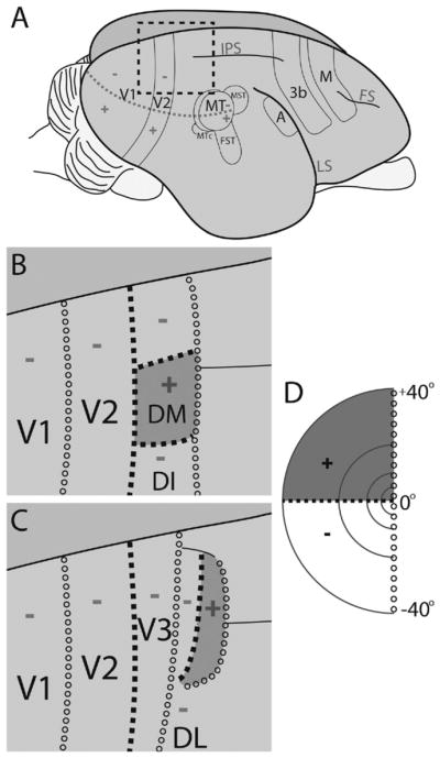
V3 versus DM. Two possible organizations of visual areas in galagos are depicted. A: Galago brain and depiction of some cortical areas. B: DM proposal: region anterior to V2 contains a full visual field representation that includes both lower and upper visual field. C: V3 proposal: region anterior to V2 is V3 and represents only ventral visual field. D: Depiction of the left visual field. DL, dorsolateral area; DI, dorsointermediate area; MT, middle temporal area; MST, middle superior temporal area; FST, fundus of superior temporal sulcus; MTc, MT crescent; A, auditory cortex; M, motor cortex; FS, frontal sulcus; LS, lateral sulcus; IPS, intraparietal sulcus. +, Upper visual field; − lower visual field; open circles, vertical meridian; filled squares, horizontal meridian.
More recently, Lyon and Kaas (2002a) provided further descriptions of the connection patterns of V1 with the extrastriate cortex in prosimian galagos, four species of New World monkeys (Lyon and Kaas, 2001, 2002c), and Old World macaques (Lyon and Kaas, 2002b) supporting the conclusion that a narrow dorsal V3, representing the lower visual quadrant, does exist between dorsal V2 and a more rostral DM (Fig. 1C). These results are strengthened by optical imaging evidence for dorsal V3 in New World owl monkeys (Lyon et al., 2002), functional magnetic resonance imaging (fMRI) evidence in macaques (Brewer et al., 2002; Tolias et al., 2005; Tehovnik et al., 2006; Schmid et al., 2009), and fMRI evidence in humans (DeYoe et al., 1996; Engel et al., 1997; Reppas et al., 1997; Tootell et al., 1997; Smith et al., 1998; Wade et al., 2002; Nishida et al., 2003).
In the present report, we provide additional evidence that a dorsal V3 lies along the rostral border of dorsal V2 in prosimian galagos. Our additional evidence is of two types. Primarily we used optical imaging of intrinsic signals to measure visually evoked cortical activity of dorsal V1, dorsal V2, and the rostrally adjoining visual cortex (Fig. 1A). The evoked pattern of activity allowed us to identify V1 and V2, and demonstrate activity along the rostral border of dorsal V2 that was evoked by stimulating the lower visual quadrant. Additionally, we recorded from neurons across the width of dorsal V1 into V2 and presumptive V3 with a 100-electrode array. The recordings demonstrate that neurons in cortex just rostral to V2 had larger receptive fields than neurons in V1 and V2, and that these receptive fields were in the lower visual quadrant, as expected for V3. Our experiments were within prosimian galagos as these primates have few cortical fissures, and thus the dorsal V1-V2-V3-DM region was accessible on the dorsal surface of the brain for optical imaging and the placement of the 100-electrode array. In addition, galagos represent the prosimian radiation, one of the major surviving branches of primate evolution, and features of cortical organization that exist across members of the early branches of primate evolution are those most likely to have been present in the early ancestors of primates (Kaas, 2004).
MATERIALS AND METHODS
Optical imaging of intrinsic signals (OIS) was used to examine the functional organization of dorsal V1, V2, and V3 in five adult galagos (Otolemur garnettii). Electrophysiological data were collected in three additional galagos. These procedures are similar to those used previously in optical imaging and electrode recording studies of visual cortex in galagos and owl monkeys (DeBruyn et al., 1993; Lyon et al., 2002; Xu et al., 2004, 2005; Kaskan et al., 2009) and single-unit recording (Jermakowicz et al., 2009). All procedures were approved by the Vanderbilt University Institute for Animal Care and Use Committee and were done in accordance with the National Institute of Health guidelines.
Animal preparation/surgery
Surgeries were performed under aseptic conditions. All galagos were initially anesthetized with ketamine hydrochloride (8–10 mg/kg) and then maintained with isofluorane (1.5–2% in O2) through an endotracheal tube during surgical procedures. Pupils were dilated by using 1% atropine eyedrops. Clear contact lenses (covered with 3-mm artificial pupils) were used to place the retina conjugate plane 28.5 cm away for imaging studies and 57 cm away for electrode recording studies. The optic discs were plotted by using a reversible ophthalmoscope or by back-reflection of the retinal blood vessel pattern from the surface of the tapetum; the area centralii were plotted based on their known relationship to the optic disc, 20° medially and 5° ventrally (Xu et al., 2005).
Anesthesia was maintained by propofol (2,6-di-isopropylphenol; induction: 3 mg/kg; maintenance: 4–10 mg/ kg/hr intravenous [i.v.]). During electrode recording studies, NO2 (NO2: 75%, O2: 23.5%, and CO2: 1.5%) was also used to maintain a stable anesthetic plane. Isofluorane was kept on standby to supplement if necessary. Paralysis was induced and maintained with vercuronium bromide mixed in 5% dextrose lactated Ringer’s solution (0.15–0.6 mg/kg/hr i.v.). The anesthetic plane of the animal was monitored by electroencephalogram during imaging experiments. Heart rate, CO2 tidal volume, and body temperature were continuously monitored throughout all experimental procedures. We regularly verified the location of the optic disc and area centralis throughout each experiment. An incision was placed along the mid-line of the scalp, and a craniotomy was performed to reveal dorsal V1, V2, and proposed V3. The brain was stabilized by using 3–4% agar with a glass coverslip for imaging studies and 1% agar for electrode array studies. We used the intraparietal sulcus as a landmark to help us locate the most likely region where V3 (or DM) would exist along the V2 border to position our imaging window. When the 100-electrode array was inserted, a large craniotomy was performed over the visual cortex centered on the representation of the area centralis around V2 (Xu et al., 2005).
Optical imaging
Images were collected by an Imager 3001 with VDAQ/ NT data acquisition software (Optical Imaging, German-town, NY). We collected intrinsic signal optical imaging data under 632-nm illumination. Images were acquired at 4 Hz for 4–8 seconds per stimulus condition (giving 16–24 frames per condition). Twenty to 50 trials were collected for each stimulus set (one block). The camera acquisition parameters were set to an image matrix of 512 × 512 with an 8 × 8-mm2 field-of-view, which yielded a 15.625 μm2 in-plane resolution.
Visual stimuli for optical imaging
High contrast square-wave gratings were created by using custom software written in Matlab (Mathworks, Natick, MA) directing a VSG stimulus system (Cambridge Research Systems, Rochester, UK). The gratings were presented in one of four orientations (0°, 45°, 90°, and 135°) on a 40 × 30-cm (displayable Width by Height) monitor in a randomly interleaved fashion. Gratings (spatial frequency 0.1–0.5 c/degree, drift velocity 2 Hz, duty cycle 20%) were drifted along the axis perpendicular to the grating orientation (in both directions). For topographic mapping, stimuli were presented to the contralateral eye with a simple cover for the ipsilateral eye or by using electromechanical shutters synchronized to the timing of stimulus presentation and image acquisition.
Coarse maps of visuotopy were made with restricted versions of the orientation gratings (either rectangular or square windows) that were presented in various locations in the visual field. The location of the center of the contralateral area centralis guided our placement of the stimuli. Heights for the rectangular windows ranged between 4° and 26° (see Figs. 4–9) with the widths spanning the screen. We typically started with the larger stimuli (20°) and then progressively used more restricted heights.
Figure 4.

Lack of upper visual field representation anterior to V2 (case 08-61). Here we present two large rectangular stimuli that were 10° apart. In each we present square wave gratings (see text). The diagrams of stimuli are for illustration purposes only and are not to scale. One stimulus is found in the lower visual field (A) and another in the upper visual field (D). In contrast to lower visual field stimulation, we found no compelling evidence for upper visual field representation along the V2 border. A: Stimulus location confined to the lower visual field (26° in height), 0° and 90° are presented. B: The resulting 8-bit gray scale orientation preference map to A. C: We created a t-map (see Materials and Methods) for the orientation preference map shown in B (P < 0.05). D: Stimulus location confined to the upper visual field (24° in height) with the same stimulus parameters as in the lower visual field confined version (A). E: The resulting 8-bit gray scale orientation preference map to D. F: As we did for the lower visual field confined map, we created a t-map from orientation preference map shown in E (P < 0.05). Solid line, V1/V2 border; dotted line, anterior V2 border; dashed line, approximate anterior border of V3. These borders are estimated based on retinotopic mapping and orientation preference maps. A, anterior; M, medial. Scale bar = 2 mm in F (applies to B,C,E,F).
Figure 9.
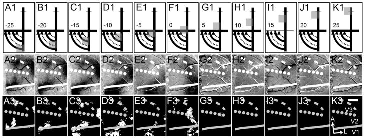
VM mapping with 10° square windows (case 10-10). Again we used 10° square stimuli but along the VM. We began in the lower visual field and moved well into the upper visual field. A1–K1: Illustration of this progression. As in Figure 8, the squares moved in 5° increments. A2–K2: The corresponding single conditions 8-bit gray scale maps. A3–K3: The corresponding t-maps (P < 0.01). There are strong activation patterns from lower visual field activation (A–E columns) but not upper field activation (G–K columns). Dashed line, presumptive anterior V3 border, estimated from this mapping; dotted line, V2/V3 border based on HM mapping from Figure 8. A, anterior; L, lateral. Scale bar = 2 mm in K3 (applies to A2-K3).
The goal of presenting stimuli within rectangular windows was to help us isolate the horizontal meridian in order to better distinguish the upper and lower visual field transition. The contralateral area centralis was replotted prior to each imaging run to check stability of eye position. To better examine the progression of the horizontal meridian (representing the anterior V2 border and possible border dividing upper and lower visual quadrants of DM) and vertical meridian (representing the V1/V2 border and the anterior border of V3 or DM), we dedicated a case to presenting 10° × 10° square-windowed stimuli (either 0° or 90° gratings, spatial frequency = 0.1 c/ degree, drift velocity = 2 Hz, duty cycle = 20%) moved in 5° steps along each meridian.
Electrode recordings
A 4 × 4-mm 100-electrode Cyberkinetics (Salt Lake City, UT) array was inserted pneumatically to a depth of about 600 μm at a location corresponding to the representation of the area centralis in V2 (Xu et al., 2005) and covering portions of V1, V2, and the proposed V3. The array was then covered with 1% agar to prevent dehydration. Receptive field location and orientation preference for each cell were determined initially by using a manually controlled bar of light projected simultaneously on a tangent screen and plotting table (DeBruyn et al., 1993).
Receptive field plotting and visual stimulation for electrode recordings
A 21-inch Sony Trinitron monitor, with refresh rate set to 120 Hz, was used to present drifting sine wave gratings. These were first presented prior to receptive field mapping to estimate locations and preferred orientations of all neurons. Eighteen 2-second trials of sine wave gratings varying in orientation (0–170° in 10° increments, 18 total) and with parameters preferred by galago visual cortex neurons (temporal frequency [TF]: 2.0 Hz, spatial frequency [SF]: 0.5 c/degree, contrast: 0.6; [DeBruyn et al., 1993]), and a gray-screen blank were presented on an 18° aperture. The drifting sine wave gratings were also used to study the neurons’ spatial and temporal frequency tuning properties. To measure SF tuning, 30 2-second trials of drifting gratings (TF: 2.0 Hz, contrast: 0.60) varying in SF (0.2–2.0 c/degree in 0.2 c/degree increments, 10 total) and orientation (0–150° in 30° increments, six total) were presented with a blank. To measure TF tuning, 30 2-second trials of drifting gratings (SF: 0.5 c/degree, contrast: 0.60) varying in TF (0.5–5.0 Hz in 10-Hz increments, 10 total) and orientation (0–150° in 30° increments, six total) were presented with a blank.
Receptive fields were plotted for all neurons that, within the 18 2-second trials of drifting orientations (see above), had clear orientation tuning with response at the preferred orientation at least twice that compared with the orthogonal orientation. Then by varying the orientation and length of a manually controlled bar of light projected simultaneously on the tangent screen and plotting table, we plotted each receptive field (DeBruyn et al., 1993). These plots, which showed each receptive field relative to the areae centralii of each eye, were then used to determine the location and size of the receptive fields.
Data analysis of optical images
Activation maps
Both single-condition maps and difference maps were calculated (Lu and Roe, 2007). Single-condition maps were either blank (isoluminant gray screen) subtracted maps or first-frame (one to two frames prior to stimulus onset) subtraction maps (frames 5–16/24 summed for better signal-to-noise). In subtraction maps, light and dark values represent preference for one condition or the other, and mid-gray values indicate equal, or no, preference for either condition. Orientation preference maps are difference maps constructed by subtracting orthogonal conditions of orientation gratings. Maps were clipped (1–2 SD[s] from the mean of the pixel distribution) and normalized to an 8-bit range. Large blood vessels were often masked to remove large signal artifact from contributing to the final clipping. In some cases, maps were low pass filtered with a Gaussian or median filter (5–8 pixels squared in size) and/or high pass filtered with a median filter (150–200 pixels squared in size).
T-maps
Significance of pixel activation was calculated by comparing images (either single-condition versus blank or two orthogonal orientation grating conditions). T-maps were calculated by conducting t-tests on a pixel-by-pixel basis by using Matlab. T-maps were visualized by creating binary maps in which pixels with P values reaching a threshold value (typically either P < 0.01 or P < 0.05) were assigned a value of one (white) and those failing to reach criterion were assigned a value of zero (black). Activation areas consisting of only a few pixels were eliminated. Significant pixels along blood vessels or along the edge of the imaging window, which are typically considered artifact due to ambiguity, were also eliminated.
Analysis of orientation patch sizes
To measure patch sizes, we used t-maps generated from orientation preference maps (either 45–135° or 90–180°). We should point out that this measurement is distinctly different from measuring the typical iso-orientation domain (e.g., Xu et al., 2004). Patch sizes were measured because we noticed that throughout our orientation preference maps there were consistent qualitative differences in patch sizes between neighboring visual areas and we wanted to see whether this difference between the neighboring visual areas was quantifiable. We chose t-maps with equal P values thresholds for all comparisons between visual areas (both across experiments and within a single experiment). To determine a patch size, we imported the t-map image into Adobe Photoshop (Adobe Systems Incorporated, San Jose, CA) and used the wand tool to select individual patches for a pixel count. We then took the provided number and multiplied it by area of a single pixel to determine its total area. Some selections appeared to be multiple patches that were connected by one or two pixels. In those cases we eliminated the connection and counted them as separate patches. Orientation patch sizes from neighboring visual areas (V1 against V2 and V2 against V3) were compared by using a Mann-Whitney U test (uncorrected).
Histological procedures
After data collection, galagos were deeply anesthetized and then given an overdose of sodium pentobarbital, and perfused transcardially with salinated 0.1 M phosphate buffer (pH 7.4) followed by 2% paraformaldehyde in 0.1 M phosphate buffer; in some cases this was followed by 2% paraphormaldehyde with 10% sucrose in 0.1 M phosphate buffer. The brain was removed and the cortex was separated from underlying brain structures and flattened as described in Krubitzer and Kaas (1990). The cortex was cut on a freezing microtome tangent to the pial surface. The cortex was cut either at a consistent thickness of 52 μm for electrophysiological cases or at a thickness of 80 μm to preserve surface vasculature for the most superficial sections, and then cut at a thickness of 40 μm for the remainder of the cortical thickness for imaging cases. Sections were then processed for cytochrome oxidase (CO) (Wong-Riley, 1979). CO stains allowed us to visualize the V1/V2 border because CO blobs terminate at the anterior border of V1. Optical images were aligned to superficial CO sections by using the surface blood vessel patterns. This alignment was facilitated with images from 568-nm illumination that highlighted surface vessel patterns collected for every in vivo imaging field-of-view used. Subsequent deeper CO sections were aligned with surface sections by using the radial blood vessels (vasculature running perpendicular to the plane of the brain sections). Electrode locations were reconstructed from holes aligned across through the serial 52-μm sections to determine their locations relative to the borders of V1, V2, and proposed V3.
RESULTS
Overview
We examined the representation of the visual field of dorsal V1, V2, and presumptive V3 in galagos. We present findings of cortical response, as measured by OIS, to 1) large upper and lower visual field stimuli; 2) restricted band stimuli; and 3) restricted square stimuli along the HM and VM. We also present electrophysiological array recordings from V1, V2, and 2 mm into our presumptive V3. In order to minimize possible contribution from eye drift, we repeatedly remapped the location of the area centralis. In both OIS and electrophysiological recordings, we found no evidence of an upper visual field representation along the dorsomedial border of V2. We describe qualitative and quantitative differences in the orientation maps among V1, V2, and V3. Estimation from imaging data of the V2/V3 border anterior to the V1/V2 border and the anterior V3 border suggests lengths ranging between 2 and 2.5 mm and 1 and 2.5 mm, respectively, consistent with the anterior–posterior extents of V2 (max ~3 mm) and V3 (max ~2.5 mm) previously reported in galagos (Collins et al., 2001; Lyon and Kaas, 2002a).
Alignment of CO-stained sections and optical images
Each experiment began with orientation mapping. As shown in Figure 2 (case 08-61), the surface vasculature revealed by CO (Fig. 2A, dashed lines) aligned with the imaged blood vessel map (Fig. 2C, dashed lines). In Figure 2B, a deeper CO section reveals the V1/V2 border (solid line) due to CO blobs in V1 and lack of CO blobs in V2. The CO section in the figure was then aligned with the superficial CO section in Figure 2A based on radial blood vessel patterns (arrows in Fig. 2A,B). The V1/V2 border defined by CO staining is consistent with that revealed in the orientation preference map (0–90° in Fig. 2D), as V2 previously has quantitatively been shown to contain larger orientation domains than V1 (Xu et al. 2005) (also see Fig. 13 and Table 1). We illustrate another example in Figure 3. As in the previous case, the V1/V2 border as shown using CO staining (Fig. 3B, solid line) is in good agreement with the V1/V2 border revealed by orientation mapping (Fig. 3D). In all subsequent figures, the V1/V2 border was determined as described for Figures 1 and 2. However, the locations of the presumptive V2/V3 and anterior V3 borders are estimates based on a combination of evidence from imaging experiments.
Figure 2.

Alignment of histological tissue and optical images (case 08-61). We used CO-stained sections to identify the location of the V1/V2 border. A: A flattened superficial CO section revealing vasculature both perpendicular (holes) and parallel to the flattened surface. B: A deeper flattened section reveals the characteristic CO blobs of V1, which terminate at the V1/V2 border (solid line). The two sections (A and B) are aligned with the vessel patterns perpendicular to the imaging plane (arrows). C: To align CO stains and our optical images, an in vivo blood vessel pattern was acquired under green light (see Materials and Methods). The dashed lines delineate sample vessels used to align with surface vasculature in the CO section (dashed lines in A). D: Optical imaging overlying V1, V2, and V3 (field-of-view is shifted from that in C; see dotted lines). V1/V2 border is then overlaid on field-of-view. Dotted line, approximate V2/V3 border; dashed line, approximate anterior border of V3. A, anterior; M, medial. Scale bar = 1 mm in A (applies to A–D).
Figure 13.
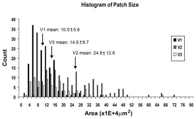
Distribution of orientation preference patch sizes in V1, V2, and V3. Patches from orientation maps for V1, V2, and V3 were measured by using t-maps at a threshold of P < 0.05. The distribution shown is pooled data from four cases. Borders for V1, V2, and V3 were chosen based on all available combinations of histological and OIS data. Mann-Whitney U tests (uncorrected) were performed in pairs: V1 versus V2 and V2 versus V3. All were found to be significantly different (P < 0.005 for all comparisons; see Table 1). V1 patches: n = 187; V2 patches: n = 157; V3 patches: n = 79.
TABLE 1.
Orientation Patch Calculations for Three Visual Areas (μm2)1
| Case | V1 (mean ± SD) | V2 (mean ± SD) | V3 (mean ± SD) | V1 vs. V2 | V2 vs. V3 |
|---|---|---|---|---|---|
| 08–07 | 10.1 ± 4.9 | 25.5 ± 14.4 | 16.4 ± 12.9 | <0.005 | <0.005 |
| 08–11 | 9.3 ± 3.5 | 30.6 ± 12.8 | 15.3 ± 6.7 | <0.005 | <0.005 |
| 08–49 | 14.8 ± 8.0 | 27.0 ± 8.0 | 11.1 ± 9.2 | <0.005 | <0.005 |
| 08–61 | 10.4 ± 5.4 | 18.4 ± 7.7 | 9.0 ± 6.0 | <0.005 | <0.005 |
| All | 10.5 ± 5.6 | 24.8 ± 12.8 | 14.5 ± 9.7 | <0.005 | <0.005 |
The mean and SDs (values listed are mean × 1E4 or SD × 1E4) of measured patches sizes for four individual cases and collectively for V1, V2, and V3 are provided. The P-values (uncorrected) for the comparisons V1 vs. V2 and V2 vs. V3 are shown based on a Mann-Whitney U test.
Figure 3.

Alignment of histological tissue and optical images (case 08-11). This is another example of aligning a CO-defined V1/V2 border to an OIS map. The V1/V2 border defined by the CO blobs overlies region of orientation patch size change. We quantify this difference later (see Figs. 12 and 13). A: A superficial CO section containing surface vasculature. B: A deeper section revealing the characteristic CO blobs of V1, which terminate at the V1/V2 border (solid line). The two sections (A and B) are aligned with vessel patterns (arrows). C: An in vivo blood vessel pattern acquired under green light (see Materials and Methods). Dashed lines delineate sample vessels used to align with surface vasculature shown (dashed lines in A). D: Orientation map in V1, V2, and area anterior to V2. Dotted line, approximate V2/V3 border; dashed line, approximate anterior border of V3. A, anterior; M, medial. Scale bar = 1 mm in C (applies to A–D).
Lower versus upper visual field representation
According to current proposals, DM has both upper and lower visual field representations, in which parts of both hemifields share a border with dorsal V2 (Fig. 1B). In our imaging experiments, oriented drifting gratings presented in the lower visual field strongly activate orientation patch regions in dorsal V1, V2, and regions directly anterior to V2, whereas the presentation of such gratings in the upper visual field does not (tested in two cases).
Figure 4 depicts data from subject 08-61 (same as Fig. 2). In response to lower visual field stimulation (Fig. 4A), orientation difference maps were obtained in V1 and V2 (Fig. 4B; t-map shown in Fig. 4C), revealing the V1/V2 border (solid line), the anterior V2 border (dotted line), and presumptive V3 spanning approximately 2 mm anterior to V2 (anterior border indicated by the dashed line). In contrast to lower field stimulation, upper field stimulation (Fig. 4D) resulted in no significant activation in V1, V2, or presumptive V3 (Fig. 4E; t-map shown in Fig. 4F). We considered the possibility that the region anterior to V2 was too weakly activated or is less orientation selective than V1 and V2. A weakness in response or orientation preference could lead to the lack of observed activity in both gray scale maps and t-maps. However examination of the t-maps at a less restrictive P value (P < 0.1) revealed no additional activation (result not shown), suggesting that the lack of activation anterior to V2 is not a consequence of inappropriate thresholding. The results indicate that V1, V2, and presumptive V3 region were all clearly activated by drifting gratings of different orientations when presented to the lower visual field, but not the upper visual field. The lack of evidence for an upper visual field representation favors the V3 interpretation anterior to dorsal V2.
Mapping with rectangular windows
We also examined retinotopic organization of these visual areas by using rectangular windows presenting oriented moving gratings. We will refer to these stimuli as bar stimuli. We conducted these experiments with 20° (two cases), 8° (three cases), and 4° (one case) bar stimuli. For these experiments we determined the location of the contralateral area centralis by using a reversible ophthalmoscope and then placed the bar stimuli parallel to the HM (see Materials and Methods).
Twenty-degree bar stimuli mapping
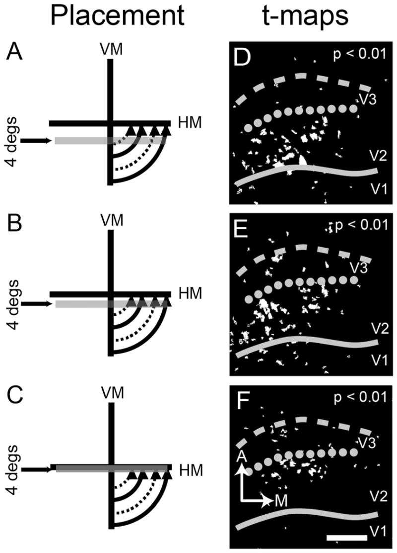
Figure 5 illustrates an experiment (case 08-11) in which 20° bar stimuli were used. Three bar stimuli (20° in height and spanning the full width of the monitor, thus crossing the vertical meridian) were placed in different locations 20–40° below the HM (Fig. 5A), 0–20° below the HM (Fig. 5B), and 0–20° above the HM (Fig. 5C). In Figure 5, the V1/V2 border (solid line) is determined from CO staining, whereas HM (dotted line) and the anterior V3 border (dashed line) were based on information gained from Figures 5, 7, and 11A/B.
Figure 5.

Retinotopic mapping with 20° bar stimuli (case 08-11). In general, we expect a medial to lateral movement as the bars move from more peripheral locations to more foveal locations. A–C: The relative stimulus (displaying 45° or 135° orientation gratings) locations for 20° height bars in the left column. D–F: The resulting t-maps (P < 0.01). As in Figure 4, the diagrams of stimulus position are purely for illustration purposes and are not to scale. Note that in C, the upper visual field stimulus shows very little activation. The pattern anterior to V2 in F overlaps with that in E, consistent with our interpretation that this is due to HM activation. Solid line, V1/V2 border, same as Figure 3; dotted line: approximate anterior V2 border based on HM mapping; dashed line, approximate anterior border of V3. A, anterior; M, medial. Scale bar = 2 mm in F (applies to D–F).
Figure 7.
Retinotopic mapping with 4° bars (case 08-11). In this case, we use a 4° bar. A–C: As in Figures 5 and 6, we show the relative position of stimuli displaying 45° and 135° gratings presented in these three spatially restricted locations. D–F: The resulting t-maps (P < 0.01). Here we see the shift toward the V2/V3 border as the bar approaches HM. Solid line, V1/V2 border, same as Figure 3; dotted line, approximate anterior V2 border based on HM mapping; dashed line, approximate anterior border of V3. A, anterior; M, medial. Scale bar = 2 mm in F (applies to D–F).
Figure 11.

Orientation preference maps are not continuous along the anterior border of V2 (cases 08-11/08-61). We show two example cases with regions that lack signal to the orientation gratings. One possibility is that this exhibits banding of orientation-selective regions in V3 (see text for additional possibilities). A,B: Gray scale orientation maps and t-maps, respectively, from case 08-11 (0°–90°). C,D: Gray scale orientation maps and t-maps, respectively, from case 08-61 (0°–90°). In contrast to V3, area V2 lacks evidence of banding. In both cases, the locations of areal borders based on banding differences between areas agrees well with the defined borders histologically and retinotopic mapping using OIS. Solid line, V1/V2 border; dotted line, V2/V3 border; dashed line, estimated anterior V3 border. A, anterior; M, medial. Scale bar = 2 mm in A (applies to A,B) and C (applies to C,D).
Within V2, we observed that as the stimulus shifted from Figure 5A to B, the cortical activation shifted from medial (Fig. 5D) to lateral (Fig. 5E). The middle bar stimulus (Fig. 5B) also revealed activation in V3; this activation spanned both the V1/V2 and the V2/V3 border, consistent with stimulation of a portion of the VM and HM, respectively. The stimulus located in the upper visual field (Fig. 5C) produced little activation in V2 and some activation in V3 (Fig. 5F). The activation observed in V3 is similar between Figure 5E and F. The similarity is likely because the stimuli placement in both Figure 5B and C interact with the HM, not due to upper visual field representation.
Based on this case alone, we cannot exclude the possibility that the activation, anterior to V2 in Figure 5F, is due to upper field activation. However, we consider this unlikely based on 1) the weakness of activation in Figure 5F compared with the robust activation in Figure 5D,E (not changed by changing t-map threshold); 2) the likelihood that the similar activation in presumptive V3 is due to common HM stimulation (Fig. 5B,E and C,F); and 3) our results from other cases (Figs. 4, 6, and 9).
Figure 6.

Retinotopic mapping with 8° bars (case 08-61). A–C: Three bars were presented here one located in the lower visual field (A), one located at the HM location (B), and one located in the upper visual field (C). As in previous figures, the diagrams are for illustration purposes only and are not to scale. Each stimulus (displaying 45° or 135° orientation gratings) was 8° in height. D–F: In the corresponding t-maps, we find activation in the lower visual field (D) and activation due to HM coverage (E) but no activation as a result of the upper visual field position (F) (P < 0.01 for all t-maps). This is consistent with the result presented in Figure 4. Solid line, V1/V2 border, same as Figure 2; dotted line, approximate anterior V2 border based on HM mapping. The estimated location of HM corresponds with that estimated in orientation map (see Fig. 11C,D). Dashed line, approximate anterior border of V3. A, anterior; M, medial. Scale bar = 2 mm in E (applies to D–F).
Eight-degree bar stimulus mapping
Results for a second experiment (case 08-61) support the interpretation presented in Figure 4 in which the cortex immediately rostral to V2 shows clear lower, but not upper, visual field activation. Figure 6A–C shows the three 8° height bar stimuli: one confined to the lower visual field (Fig. 6A), one spanning the HM (Fig. 6B), and one confined to the upper visual field (Fig. 6C). The restricted lower field stimulations elicited clear activation in V1 and V2 (Fig. 6D). The stimulus spanning the HM activated more lateral regions of V1 and V2, consistent with representation of central vision. It also produced activation in V3 and along the V2/V3 border (dotted line of Fig. 6E). Most importantly, the upper field stimulus (Fig. 6C) produced no activation in V1, V2, or the region anterior to V2 (Fig. 6F). The location of the presumptive V2/V3 border, as determined from HM stimulus mapping, was about 2–2.5 mm anterior to the V1/V2 border. The results for Figures 4 and 6 show a distinct lack of upper visual field representation, making it unlikely that the activation in Figure 5F contains an upper visual field component.
Four-degree bar stimulus mapping
In a third experiment, we used smaller 4° bar stimuli to try to increase our precision (Fig. 7A–C, case 08-11, the same case as Fig. 5 but slightly different field-of-view). This is the only case in which maps from 4° bar stimuli were obtained. As observed in the t-maps (P < 0.01; Fig. 7D,E), significant activation was observed within V2, with the pattern of activation shifting toward the V2/V3 border as the stimulus shifted upward toward the HM (Fig. 7A to B to C). The stimulus that overlies the HM (Fig. 7C) elicited activation largely at the V2/V3 border (dotted line of Fig. 7D–F).
Mapping with square windows
In one case (case 10-10), we used restricted 10 × 10° windows presenting oriented gratings (0° or 90°) moved in 5° steps along the HM (Fig. 8) and the VM (Fig. 9). Figure 8A1–E1 illustrates visual stimulus positions progressively moved from central to peripheral locations. As shown by the activation maps in gray scale (Fig. 8A2–E2) and in t-map (Fig. 8A3–E3) form, the activation pattern shifts from lateral (Fig. 8A2/3) to medial (Fig. 8E2/3) in V2 (between solid line and dotted line) along the representation of the horizontal meridian (dotted line). The dotted line was placed based on images in Figure 8C2/3–E2/3 and extrapolated medially. Note that the largest area of cortical activation in V1, V2, and V3 is seen with centrally located stimuli (Fig. 8A3–B3) and declines with more eccentric stimuli (Fig. 8C3–E3).
Figure 8.

HM mapping with 10° square windows (case 10-10). Here we used 10° square windowed stimuli along the HM. A1–E1: Illustration of the relative positions of the squares. The stimuli start at the area centralis and move in 5° increments into the periphery. Here we used single condition maps (see Materials and Methods) to visualize the cortical representation. A2–E2: The familiar 8-bit gray scale images. A3–E3: Corresponding t-maps (P < 0.01). See text for additional details. Solid line, V1/V2 border; dotted line, V2/V3 border based on this HM mapping; dashed line, presumptive anterior V3 border, estimated from VM mapping shown in Figure 9. A, anterior; L, lateral. Scale bar = 2 mm in E3 (applies to A2–E3).
We used the same mapping procedure along the VM. Figure 9 provides further evidence (displayed as single-conditions maps) that the cortex immediately anterior to V2 is not responsive to upper visual field stimulus but is responsive to the same stimuli in the lower visual field. As the visual stimulus moved from peripheral (lower field, Fig. 9A1) to central locations (Fig. 9F1; stimulus locations shown in Fig. 9A1–K1), the activation (single-condition maps shown in Fig. 9A2–K2 and t-maps shown in Fig. 9A3–K3) traveled from medial (Fig. 9A2/A3) to lateral (Fig. 9F2/F3) along the cortex, providing an estimate of the location of the VM representation at both the V1/V2 (solid line) and the anterior V3 (dashed line) borders. Interestingly, we also see another VM activation anterior to V2 along the lateral margin of our imaged cortex that we think is likely DL (V4). The pattern is easily seen in Figure 9A3–C3 just lateral to the dotted and dashed lines. At the HM/VM intersection (Fig. 9F1), we see activation laterally in V1, V2, and V3. Note that the central most stimulus (Fig. 9F1) is very similar to that seen in Figure 8A1. Importantly, no significant activation is observed in response to upper field stimuli (Fig. 9G–K).
Electrophysiology
To further investigate the organization of the cortex in the region of presumptive V3, we recorded from three galagos with a 4 × 4 mm2 100-electrode Cyberkinetics array placed over a location similar to our imaged area. A total of 175 well-isolated singe units were recorded from V1, V2, and presumptive V3. Figure 10 summarizes results from case 07-12. V1 neurons were distinguished by their location within the CO blob region (Fig. 10A). V2 neurons were located in a band of cortex corresponding to the known width of V2 just rostral to V1. The receptive fields of V2 neurons were consistently larger than those for V1 neurons, data that are consistent with the larger orientation domains demonstrated with optical imaging within V2 (Xu et al., 2005). As shown in Figure 10B, the presumptive V3 neurons were distinguished by considerably larger receptive fields than V2 neurons (mean ± SE; V2: 12.3 ± 2.5 degree2, V3: 138 ± 22 degree2; P < 0.05; uncorrected Mann-Whitney U test). Figure 10C shows positions along an exemplar set of pins in a recording session. The receptive field progression for the labeled pins (A–G) in Figure 10C is displayed in Figure 10D where the increase in receptive field size between V2 and V3 is clear. All presumptive V3 neurons were recorded at a distance of 1.5 mm or greater, anterior to the edge of the V1 CO blobs.
Figure 10.

Electrode array recording data. A: CO-stained section of visual cortex after removal of the array. The V1/V2 border was determined by using CO staining to mark CO blobs in area V1. Red dots, V1 electrodes; green dots, V2 electrodes; blue dots, V3 electrodes. A, anterior; D, dorsal. B: Receptive fields of 56 V1, V2, and V3 neurons. The V2/V3 border was determined by dramatic change in receptive field sizes. Red, V1; green, V2; Blue, V3. C: Schematic of 10 pins and their relative locations in V1, V2, and V3. D: Receptive field locations on selected pins within a 10-pin row along the array. The greater receptive field size in V3 allows the three-pin progression in V3 to span nearly the entire arc from the VM to HM. E: Average spatial frequency preference of the 56 neurons from this case. F: Average temporal frequency preference of the 56 neurons from this case. Scale bar = 1 mm in A; 2° in B and D.
This classification yielded 69 V1 neurons, 51 V2 neurons, and 55 V3 neurons. Additionally, clear differences existed between the average preferred spatial frequency (P < 0.05, ANOVA; mean ± SE; V1: 0.607 ± 0.024 c/ degree, V2: 0.547 ± 0.03 c/degree, V3: 0.431 ± 0.038 c/degree; Fig. 10E) and the average preferred temporal frequency (P < 0.05, ANOVA; mean ± SE; V1: 1.84 ± 0.10 Hz, V2: 2.32 ± 0.11 Hz, V3: 2.49 ± 0.13 Hz; Fig. 10F) of the neurons divided into these groups, further indicating that neurons with these receptive field properties came from different visual areas. V1 neurons preferred the highest spatial and lowest temporal frequencies whereas the presumptive V3 neurons preferred the lowest spatial and highest temporal frequencies.
Most importantly, consistent with a V3 interpretation, all of the proposed V3 receptive field centers fell within the lower visual field (Fig. 10B, blue squares). The retinotopic distributions of V1, V2, and V3 receptive fields observed in case 07-12 are representative of all three cases (Fig. 10B). In these cases, the V3 receptive fields extended from the HM to 10–15° below the horizontal meridian, overlapping nearly all of the dorsal V1 and V2 receptive fields.
Although some of the V3 receptive fields impinge on the upper field representation, the receptive field centers are clearly in the lower field. The receptive field labeled E in Figure 10D provides an example of where receptive fields that impinge on the upper visual field can be found. Moreover, as seen from the imaging evidence (Figs. 4–9), any such impingement on the upper field reveals no associated cortical activation. The large receptive field sizes and scatter also help explain why a clear retinotopic progression is challenging to obtain in galagos. In only three pins, the receptive fields labeled E to G in V3 (Fig. 10C,D) involve some part of the HM (pin E in Fig. 10C,D) and encroach on VM (pin G in Fig. 10C,D).
Orientation patch sizes in V1, V2, and V3
Another way to differentiate areas is based on differences in functional organization and patch size. We found both qualitative and quantitative differences in orientation structure between V2 and V3. Figure 11 shows orientation preference maps from two cases (Fig. 11A,B and C,D) in which the V2/V3 borders (dotted lines) were estimated by the available OIS data described above. Orientation maps in V2 appear continuous, consistent with previous observations (Xu et al., 2005). However, V3 reveals a discontinuous or banded appearance (Fig. 11B,D). This discontinuous appearance in V3 is also evident in Figures 4C, 5E, and 6E. This is reminiscent of previous descriptions in owl monkey V3 (Kaskan et al., 2009; Xu et al., 2004). We did not conduct additional studies to determine what bearing on retinotopic maps the banding causes. We did attempt other stimulus features (such as moving random dots [Lu et al., 2010] and large field luminance modulation [(Kaskan et al., 2009]) to see whether we could elicit responses other than orientation selectivity or possible complementary structure; however, these stimuli did not reveal any significant cortical responses.
Throughout our images, by qualitative assessment, orientation preference patches were noticeably different between neighboring visual areas. Because we noticed this difference in the orientation difference maps, we investigated the difference in this form. Figure 12 (case 08-49) illustrates our procedure for measuring orientation patch sizes in V2 and V3. Because we did not want to make any a priori assumption about the location of the V2/V3 border, we developed an iterative procedure, which identified a border between two regions of significantly different patch sizes (P < 0.05). To do this, we used 1-mm-wide zones (shaded rectangles in Fig. 12E) anterior to the V1/V2 border and measured patch sizes (based on t-maps of orientation difference maps) in each of these zones. We repeated this procedure, shifting the two zones in 0.25-mm increments from near the V1/V2 border through the V3 region. Through this procedure, we identified the border location, which yielded the maximal difference in patch sizes (the smallest P value). We also tested smaller 0.1-mm increments but found little difference in the final location. The dotted line in Figure 12F reflects the position determined for this case. There is no retinotopic mapping associated with this line; the dotted line simply marks the location dividing regions of orientation patch size difference. Its position is an approximation of where the V2/V3 border lies. We also examined patch size distributions based on qualitative estimation of V2/ V3 borders and found no difference in resulting distributions.
Figure 12.

Procedure for orientation preference patch size determination (case 08-49). In many of the orientation preference maps, it appeared that there were three distinct populations of orientation patch sizes. A: A superficial CO section containing surface vasculature. B: A deeper section revealing the characteristic CO blobs of V1, which terminate at the V1/V2 border (solid line). C: An in vivo blood vessel pattern acquired under green light (see Materials and Methods). Dashed lines in A and C delineate sample vessels used to align with surface vasculature shown. D: Orientation map in V1, V2, and area anterior to V2. As in Figures 3 and 4, we used this information (A–D) to place the CO blob defined V1/V2 border onto our imaging maps. E,F: T-map (P < 0.05) of the orientation preference map shown in D. We determined those samples by using two sample regions (the superimposed light gray rectangles 1 mm in height). The bars were moved in an iterative fashion to arrive at this final location (see text). Only those patches lying within a single sample region were selected for measurement. Solid line, V1/V2 border; dotted line, estimated V2/V3 border; dashed line, estimated anterior V3 border. A, anterior; M, medial. Scale bar = 1 mm in C (applies to A–F).
Figure 13 shows the distributions of orientation patch sizes in V1 (n = 187), V2 (n = 157), and V3 (n = 79) pooled from four cases for 10 total difference maps (three cases contributed one hemisphere, and one case contributed both hemispheres). For each hemisphere, we measured patches for two maps within the orientation preference t-map of orthogonal conditions (45–135° and 90–180°). The patch sizes in V1 were taken from the region of the cortex characterized by V1 cytochrome oxidase staining. Those in V2 and V3 were taken via the process described previously. Means and SDs are indicated. The same P values were used for all t-maps. We did not remove outliers and included all values. Removing outliers (greater than 2 SDs) did improve our statistics, but did not change the location of borders. We used a Mann-Whitney U test (uncorrected) to compare patch sizes in V1 versus V2 and V2 versus V3. All comparisons were significantly different (all P < 0.005). The differences between V1 and V2 and between V2 and V3 were significant within each case as well as across cases (Table 1). Surprisingly, V3 did not possess the largest orientation preference patch sizes, but was intermediate in patch size between V1 and V2.
DISCUSSION
Summary
In this study, we used OIS and electrophysiology to examine the cortical representation anterior to area V2 in prosimian galagos. We find little evidence for an upper field representation in this region, suggesting that, in galagos, the cortex anterior to V2 is area V3 and not area DM. By using OIS we studied six hemispheres in five galagos. The main OIS findings were: 1) lack of upper field activation anterior to V2; 2) VM representation at the V1/ V2 border and the anterior V3 border; 3) one HM representation dividing V2 and V3; 4) a lateral to medial shift in cortical activation with greater stimulus eccentricity, consistent with previous mapping studies; 5) a V2/V3 border 1.5–2.5 mm anterior to the V1/V2 border and an anterior V3 border 1–2.5 mm further anterior, consistent with the anterior–posterior extents of V2 (max ~3 mm) and V3 (max ~2.5 mm) reported previously in galagos (Collins et al., 2001; Lyon and Kaas, 2002a); 6) distinctions among V1, V2, and V3 by orientation preference patch size; and 7) possible banding structure in V3. In addition to our OIS findings, we provide receptive field mapping data, in three additional galagos, from 100-electrode array recording, illustrating three distinct pools of receptive field sizes, average spatial frequency preference, and average temporal frequency preference in V1, V2, and V3, none of which exhibited an upper field representation, consistent with the OIS data. These findings thus suggest that the region anterior to V2 is area V3 and provide no compelling evidence for a DM representation.
Experimental considerations
In this study, we found no evidence for an upper visual field representation in the region anterior to V2. This is curious given reports of an upper visual field representation bordering V2 (Allman et al., 1979; Krubitzer and Kaas, 1993; Rosa and Schmid, 1995; Beck and Kaas, 1998a,b; Rosa et al., 1997, 2000, 2005, 2009; Rosa and Tweedale, 2000, 2005). Here, we discuss experimental considerations.
One possibility is that the lack of upper field response was due to general ineffectiveness of the stimuli presented. However, this seems unlikely. Using the same experimental conditions, we consistently elicited clear activation throughout the imaging field-of-view with lower visual field stimuli. To examine whether the upper visual field representation was present but weaker, we assessed the activation maps at lower P value thresholds but still failed to find upper field activation. In contrast, stimuli falling on the HM or in the lower visual field demonstrate clear activation (Figs. 2–9). Consistent results were obtained with full field, rectangular, and square windowed stimuli, indicating that the lack of upper visual field activation is not due to stimulus size or configuration. Additionally, under similar anesthesia protocols, these same stimuli elicited clear electrophysiological mapping of receptive fields (Fig. 10) in the lower visual field but not the upper visual field.
It is also unlikely that our imaging field-of-view or electrophysiology array failed to include the area of interest. Our imaging field-of-view was quite large (8 × 8 mm) and included not only V1 and V2, but also the additional several millimeters anterior to V2. We also confirmed histologically that the electrophysiology array spanned several millimeters anterior to the V1/V2 border. With respect to mediolateral extent, our field-of-view extended from medial to fairly lateral (foveal) regions of cortex. We also used the intraparietal sulcus as an anatomical landmark (see Materials and Methods), and are sure that our sampling areas included the relevant cortex in question near the anterior border of dorsal V2.
Another potential source of error is in our estimate of the area centralis location. This could lead to the false assignment of upper visual field representation to the lower field. However, we find this unlikely as we repeatedly measured the area centralis location prior to each imaging run and due to our paralytic the position was very stable throughout experimentation. We also tested locations well into the upper visual field and found no upper field representation. Additionally, the estimated locations of the horizontal and vertical meridian were consistent across experiments and consistent with the size of V2 from previous studies. Thus, despite significant efforts, we were unable to find any evidence for an upper field representation anterior to V2.
A final concern is the focal plane. We devote significant effort to minimizing this concern for all optical imaging studies conducted. There are several techniques and strategies we use to minimize this issue. With these techniques, it has been shown that we can achieve reasonable flattening over quite large field-of-views (~2 cm; cf. Lu et al., 2010). We also take great pains to align the plane of the camera with the imaging plane of the window. Evidence of our ability to obtain a high quality of our focal plane is shown in the vessel images acquired under green light (Figs. 2, 3, 12). Note that only local indentations in the cortex (intraparietal sulcus in the upper anterior potions of Figs. 2C and 3C, and a dimple that appears in some galago visual cortex in the caudal–medial parts of Fig. 12C) appear slightly out of focus; however, even these regions are not obviously different. We often also obtain more than one imaging field-of-view for a single subject, as in some runs we shift the field-of-view more anteriorly to capture more V2 and V3 (e.g., see Fig. 11A and compare with Fig. 3D). Thus we often replicate results within a single subject with more than one field-of-view and still obtain similar results. We will also perform high-pass filtering to minimize effects of uneven illumination. It should also be noted that we base our final interpretations on statistical t-maps, which further minimize concerns due to any slight differences in cortical curvature. Thus, we are quite confident that any lack of activation observed in V3 is not due to effects of out of focus cortex.
Consistent with dorsal V3
Optical imaging evidence in owl monkeys (Kaskan et al., 2009; Lyon et al., 2002; Xu et al., 2004) and some tracer studies in New World monkeys (Lyon and Kaas, 2001, 2002c) support the interpretation that dorsal V3 (depicted in Fig. 1C) lies along the rostral border of dorsomedial V2. However there continues to be electrophysiology and some tracer studies supporting the presence of DM (depicted in Fig. 1C) along V2, instead of dorsal V3 (Rosa and Schmid, 1995; Lui et al., 2006; Jeffs et al., 2012; Rosa et al., 2000, 2005, 2009; Rosa and Tweedale, 2000, 2001, 2005). In prosimians, early electrode recording and anatomical studies also suggest the representation of the upper visual field directly along the anterior border of dorsal V2 (Allman et al., 1979; Newsome and Allman, 1980; Rosa et al., 1997; Beck and Kaas, 1998b). However a reinvestigation of the connection patterns in galagos, by using tracers placed in V1, supported the existence of a V3 in prosimians (Lyon and Kaas, 2002a). The ability for Lyon and Kaas (2001, 2002a–c) to detect V3 by using tracer studies in a variety of primates is partly due to strategy. By making targeted injections of refined tracers into V1, Lyon and Kaas were able to clearly confine injections into a single visual area.
The combined optical imaging and electrophysiological evidence in this study was extremely important considering that a significant part of the interpretational division lies along methodological lines. Electrode recordings have tended to favor a DM interpretation (Rosa and Tweedale, 2000; Rosa et al., 2009). However, given the large size of receptive fields anterior to V2, single penetration electrophysiological mapping may not provide sufficient density or positional certainty to map reversals. The use of fixed arrays of microelectrodes alleviates much of the positional ambiguity. The difficulty of interpretation is highlighted by Lyon and Connolly (2012) in their argument for V3 in primates, where they demonstrate that electrophysiology data previously published in favor of DM can easily be reinterpreted to support the existence of V3. Based on the retinotopic data provided in Figures 5–9, a mirror reflection between V2 and V3 is only an approximation. It seems that central visual field representations appear more dominant than peripheral representations (except see Fig. 9) in V3. However, the weakness of peripheral representation could be due to a banded organizational scheme in V3 (see next subsection, Functional organization). Another reported aspect of the DM hypotheses is the existence of an HM representation perpendicular to the HM along the anterior border of dorsal V2 (Fig. 1B). However, the evidence presented provides no support for such an HM representation.
Functional organization
We confirm previous reports of orientation-selective responses anterior to dorsal V2 in the presumptive area V3 of galagos (Jermakowicz et al., 2009). We also demonstrate the ability to distinguish V1, V2, and V3 based on their relative orientation preference patch sizes (Figs. 12, 13) and the sizes of individually mapped receptive fields (Fig. 10). Consistent with previous studies on iso-orientation domains in owl monkeys (Xu et al., 2004) and in galagos (Xu et al., 2005), we find that orientation patch sizes in V2 are larger than those in V1. Surprisingly, orientation patch sizes appear to be smaller in V3 than in V2 in the galago. This is in contrast to iso-orientation domains in the owl monkeys, which are larger in V3 than in V1 or V2 (Xu et al., 2004). However this relationship could change if we were to calculate the relationships between iso-orientation domains rather than patches. Iso-orientation comparisons in owl monkeys (Xu et al., 2004) showed the V2 and V3 iso-orientation distinction to be small and not significantly different. Ultimately we chose not to pursue iso-orientation measures because we were interested in a quantifiable difference. It would be more interesting to see if using orientation patch size between V2 and V3 from simple difference maps produced significant differences in primates where iso-orientation domain sizes were not statistically significant. Being able to distinguish visual areas by using difference maps of orientation preference would allow for quick assessment of visual area borders without explicit visuotopic mapping, which would be advantageous for several applications. We highlight two interesting points using our simplified differentiation. First, the qualitative difference between the neighboring visual areas is quantifiable (Figs. 12, 13). Second, the locations for these borders are similar in location to those found by more traditional mapping.
Consistent with a previous study (Xu et al., 2004), V2 in galagos lacks any band-like structure, unlike that in the macaque (Roe and Ts’o, 1995; Lu and Roe, 2007, 2008), owl monkey (Kaskan et al., 2009; Xu et al., 2004), or marmoset (Roe et al., 2005, McLoughlin and Schiessl, 2006; Federer et al., 2009), in which there is a clear presence of a band-like appearance, associated with high and low orientation selectivity. We found orientation maps that appear band-like in galago V3 (Fig. 11). This is reminiscent of the bands described in owl monkey V3 (Xu et al., 2004; Kaskan et al., 2009).
We report the first evidence of possible banding in presumptive V3 in galagos. To investigate the possibility that the regions between the orientation bands may have different stimulus preference, we used other stimuli (e.g., moving dot stimuli, full-field luminance modulation) but did not observe activation to these stimuli. Alternatively, patches of V3 may become unresponsive under our particular mapping conditions. One interesting possibility to consider is that the gaps between the bands represent an intrusion of another visual area into the proposed V3 region. If present, our study suggests that its functional properties would be asymmetrical to the proposed V3. Previously, Rosa et al. (2005; see their Fig. 17B) considered such a model but dismissed it because of its complexity. Our data do not eliminate this possibility.
CONCLUSIONS
V3 can be found in a variety of primate species based on V1 connections and architectural features (Lyon and Kaas, 2001, 2002a–c). From the current study and in previous studies, optical imaging of intrinsic signal has provided functional evidence for dorsal V3 in prosimian and New World primates (Lyon et al., 2002; Xu et al., 2004; Kaskan et al., 2009). Electrode recordings anterior to V2 also suggest the existence of V3 in macaques (Zeki, 1978a,b; Baizer, 1982; Felleman and Van Essen, 1987; Gattass et al., 1988; Poggio et al., 1988; Adams and Zeki, 2001). Human (DeYoe et al., 1996; Engel et al., 1997; Reppas et al., 1997; Tootell et al., 1997; Smith et al., 1998; Wade et al., 2002; Nishida et al., 2003) and macaque fMRI (Brewer et al., 2002; Tolias et al., 2005; Tehovnik et al., 2006; Schmid et al., 2009) studies also appear more consistent with a V3 interpretation.
In this study, we provide the first OIS data regarding the visuotopy of the cortical area anterior to V2 in galagos and confirm that receptive fields in this zone are much larger than in either V1 or V2. We also present the first OIS evidence for orientation preference maps in galago V3, demonstrate differences in orientation patch sizes in V1, V2, and V3, and suggest possible band-like functional architecture within V3. Finally, the lack of detectable upper visual field representation suggests that this area is more consistent with V3, not DM, and argues in favor of the inclusion of V3 as a common visual area among primates.
Acknowledgments
Grant sponsor: National Institutes of Health; Grant numbers: EY11744, EY002686, EY01778, EY007135, P30-EY08126 and P30-HD015052.
We thank Lisa Chu, Julia Mavity-Hudson, Alyssa Zuehl, Dr. Robert Friedman, and Dr. Haidong Lu for all their valuable assistance and thoughtful discussions.
LITERATURE CITED
- Adams DL, Zeki S. Functional organization of macaque V3 for stereoscopic depth. J Neurophysiol. 2001;86:2195–2203. doi: 10.1152/jn.2001.86.5.2195. [DOI] [PubMed] [Google Scholar]
- Allman JM, Kaas JH. The dorsomedial cortical visual area: a third tier area in the occipital lobe of the owl monkey (Aotus trivirgatus) Brain Res. 1975;100:473–487. doi: 10.1016/0006-8993(75)90153-5. [DOI] [PubMed] [Google Scholar]
- Allman J, Campbell CB, McGuinness E. The dorsal third tier area in Galago senegalensis. Brain Res. 1979;179:355–361. doi: 10.1016/0006-8993(79)90450-5. [DOI] [PubMed] [Google Scholar]
- Baizer JS. Receptive field properties of V3 neurons in monkey. Invest Ophthalmol Vis Sci. 1982;23:87–95. [PubMed] [Google Scholar]
- Beck PD, Kaas JH. Cortical connections of the dorsomedial visual area in new world owl monkeys (Aotus trivir-gatus) and squirrel monkeys (Saimiri sciureus) J Comp Neurol. 1998a;400:18–34. doi: 10.1002/(sici)1096-9861(19981012)400:1<18::aid-cne2>3.0.co;2-w. [DOI] [PubMed] [Google Scholar]
- Beck PD, Kaas JH. Cortical connections of the dorsomedial visual area in prosimian primates. J Comp Neurol. 1998b;398:162–178. [PubMed] [Google Scholar]
- Brewer AA, Press WA, Logothetis NK, Wandell BA. Visual areas in macaque cortex measured using functional magnetic resonance imaging. J Neurosci. 2002;22:10416–10426. doi: 10.1523/JNEUROSCI.22-23-10416.2002. [DOI] [PMC free article] [PubMed] [Google Scholar]
- Collins CE, Stepniewska I, Kaas JH. Topographic patterns of v2 cortical connections in a prosimian primate (Galago garnettii) J Comp Neurol. 2001;431:155–167. [PubMed] [Google Scholar]
- Cragg BG. The topography of the afferent projections in the circumstriate visual cortex of the monkey studied by the Nauta method. Vision Res. 1969;9:733–747. doi: 10.1016/0042-6989(69)90011-x. [DOI] [PubMed] [Google Scholar]
- DeBruyn EJ, Casagrande VA, Beck PD, Bonds AB. Visual resolution and sensitivity of single cells in the primary visual cortex (V1) of a nocturnal primate (bush baby): correlations with cortical layers and cytochrome oxidase patterns. J Neurophysiol. 1993;69:3–18. doi: 10.1152/jn.1993.69.1.3. [DOI] [PubMed] [Google Scholar]
- DeYoe EA, Carman GJ, Bandettini P, Glickman S, Wieser J, Cox R, Miller D, Neitz J. Mapping striate and extrastriate visual areas in human cerebral cortex. Proc Natl Acad Sci U S A. 1996;93:2382–2386. doi: 10.1073/pnas.93.6.2382. [DOI] [PMC free article] [PubMed] [Google Scholar]
- Engel SA, Glover GH, Wandell BA. Retinotopic organization in human visual cortex and the spatial precision of functional MRI. Cereb Cortex. 1997;7:181–192. doi: 10.1093/cercor/7.2.181. [DOI] [PubMed] [Google Scholar]
- Federer F, Ichida JM, Jeffs J, Schiessl I, McLoughlin N, Angelucci A. Four projection streams from primate V1 to the cytochrome oxidase stripes of V2. J Neurosci. 2009;29:15455–15471. doi: 10.1523/JNEUROSCI.1648-09.2009. [DOI] [PMC free article] [PubMed] [Google Scholar]
- Felleman DJ, Van Essen DC. Receptive field properties of neurons in area V3 of macaque monkey extrastriate cortex. J Neurophysiol. 1987;57:889–920. doi: 10.1152/jn.1987.57.4.889. [DOI] [PubMed] [Google Scholar]
- Felleman DJ, Van Essen DC. Distributed hierarchical processing in the primate cerebral cortex. Cereb Cortex. 1991;1:1–47. doi: 10.1093/cercor/1.1.1-a. [DOI] [PubMed] [Google Scholar]
- Gattass R, Sousa AP, Gross CG. Visuotopic organization and extent of V3 and V4 of the macaque. J Neurosci. 1988;8:1831–1845. doi: 10.1523/JNEUROSCI.08-06-01831.1988. [DOI] [PMC free article] [PubMed] [Google Scholar]
- Jeffs J, Federer F, Ichida JM, Angelucci A. High-Resolution Mapping of Anatomical Connections in Marmoset Extrastriate Cortex Reveals a Complete Representation of the Visual Field Bordering Dorsal V2. Cereb Cortex. 2012 Apr 20; doi: 10.1093/cercor/bhs088. [Epub ahead of print] [DOI] [PMC free article] [PubMed] [Google Scholar]
- Jermakowicz WJ, Chen X, Khaytin I, Bonds AB, Casagrande VA. Relationship between spontaneous and evoked spike-time correlations in primate visual cortex. J Neurophysiol. 2009;101:2279–2289. doi: 10.1152/jn.91207.2008. [DOI] [PMC free article] [PubMed] [Google Scholar]
- Kaas JH. Neuroanatomy is needed to define the “organs” of the brain. Cortex. 2004;40:207–208. doi: 10.1016/s0010-9452(08)70952-3. [DOI] [PubMed] [Google Scholar]
- Kaskan PM, Lu HD, Dillenburger BC, Kaas JH, Roe AW. The organization of orientation-selective, luminance-change and binocular- preference domains in the second (V2) and third (V3) visual areas of New World owl monkeys as revealed by intrinsic signal optical imaging. Cereb Cortex. 2009;19:1394–1407. doi: 10.1093/cercor/bhn178. [DOI] [PMC free article] [PubMed] [Google Scholar]
- Krubitzer LA, Kaas JH. Cortical integration of parallel pathways in the visual system of primates. Brain Res. 1989;478:161–165. doi: 10.1016/0006-8993(89)91490-x. [DOI] [PubMed] [Google Scholar]
- Krubitzer LA, Kaas JH. Cortical connections of MT in four species of primates: areal, modular, and retinotopic patterns. Vis Neurosci. 1990;5:165–204. doi: 10.1017/s0952523800000213. [DOI] [PubMed] [Google Scholar]
- Krubitzer LA, Kaas JH. The dorsomedial visual area of owl monkeys: connections, myeloarchitecture, and homologies in other primates. J Comp Neurol. 1993;334:497–528. doi: 10.1002/cne.903340402. [DOI] [PubMed] [Google Scholar]
- Lu HD, Roe AW. Optical imaging of contrast response in Macaque monkey V1 and V2. Cereb Cortex. 2007;17:2675–2695. doi: 10.1093/cercor/bhl177. [DOI] [PubMed] [Google Scholar]
- Lu HD, Roe AW. Functional organization of color domains in V1 and V2 of macaque monkey revealed by optical imaging. Cereb Cortex. 2008;18:516–533. doi: 10.1093/cercor/bhm081. [DOI] [PMC free article] [PubMed] [Google Scholar]
- Lu HD, Chen G, Tanigawa H, Roe AW. A motion direction map in macaque V2. Neuron. 2010;68:1002–1013. doi: 10.1016/j.neuron.2010.11.020. [DOI] [PMC free article] [PubMed] [Google Scholar]
- Lui LL, Bourne JA, Rosa MG. Functional response properties of neurons in the dorsomedial visual area of New World monkeys (Callithrix jacchus) Cereb Cortex. 2006;16:162–177. doi: 10.1093/cercor/bhi094. [DOI] [PubMed] [Google Scholar]
- Lyon DC, Connolly JD. The case for primate V3. Proc Biol Sci. 2012;279:625–633. doi: 10.1098/rspb.2011.2048. [DOI] [PMC free article] [PubMed] [Google Scholar]
- Lyon DC, Kaas JH. Connectional and architectonic evidence for dorsal and ventral V3, and dorsomedial area in marmoset monkeys. J Neurosci. 2001;21:249–261. doi: 10.1523/JNEUROSCI.21-01-00249.2001. [DOI] [PMC free article] [PubMed] [Google Scholar]
- Lyon DC, Kaas JH. Connectional evidence for dorsal and ventral V3, and other extrastriate areas in the prosimian primate, Galago garnettii. Brain Behav Evol. 2002a;59:114–129. doi: 10.1159/000064159. [DOI] [PubMed] [Google Scholar]
- Lyon DC, Kaas JH. Evidence for a modified V3 with dorsal and ventral halves in macaque monkeys. Neuron. 2002b;33:453–461. doi: 10.1016/s0896-6273(02)00580-9. [DOI] [PubMed] [Google Scholar]
- Lyon DC, Kaas JH. Evidence from V1 connections for both dorsal and ventral subdivisions of V3 in three species of New World monkeys. J Comp Neurol. 2002c;449:281–297. doi: 10.1002/cne.10297. [DOI] [PubMed] [Google Scholar]
- Lyon DC, Xu X, Casagrande VA, Stefansic JD, Shima D, Kaas JH. Optical imaging reveals retinotopic organization of dorsal V3 in New World owl monkeys. Proc Natl Acad Sci U S A. 2002;99:15735–15742. doi: 10.1073/pnas.242600699. [DOI] [PMC free article] [PubMed] [Google Scholar]
- McLoughlin N, Schiessl I. Orientation selectivity in the common marmoset (Callithrix jacchus): the periodicity of orientation columns in V1 and V2. Neuroimage. 2006;31:76–85. doi: 10.1016/j.neuroimage.2005.12.054. [DOI] [PubMed] [Google Scholar]
- Newsome WT, Allman JM. Interhemispheric connections of visual cortex in the owl monkey, Aotus trivirgatus, and the bushbaby, Galago senegalensis. J Comp Neurol. 1980;194:209–233. doi: 10.1002/cne.901940111. [DOI] [PubMed] [Google Scholar]
- Nishida S, Sasaki Y, Murakami I, Watanabe T, Tootell RB. Neuroimaging of direction-selective mechanisms for second-order motion. J Neurophysiol. 2003;90:3242–3254. doi: 10.1152/jn.00693.2003. [DOI] [PubMed] [Google Scholar]
- Poggio GF, Gonzalez F, Krause F. Stereoscopic mechanisms in monkey visual cortex: binocular correlation and disparity selectivity. J Neurosci. 1988;8:4531–4550. doi: 10.1523/JNEUROSCI.08-12-04531.1988. [DOI] [PMC free article] [PubMed] [Google Scholar]
- Reppas JB, Niyogi S, Dale AM, Sereno MI, Tootell RB. Representation of motion boundaries in retinotopic human visual cortical areas. Nature. 1997;388(6638):175–179. doi: 10.1038/40633. [DOI] [PubMed] [Google Scholar]
- Roe AW, Ts’o DY. Visual topography in primate V2: multiple representation across functional stripes. J Neurosci. 1995;15:3689–3715. doi: 10.1523/JNEUROSCI.15-05-03689.1995. [DOI] [PMC free article] [PubMed] [Google Scholar]
- Roe AW, Fritsches K, Pettigrew JD. Optical imaging of functional organization of V1 and V2 in marmoset visual cortex. Anat Rec A Discov Mol Cell Evol Biol. 2005;287:1213–1225. doi: 10.1002/ar.a.20248. [DOI] [PubMed] [Google Scholar]
- Rosa MG, Schmid LM. Visual areas in the dorsal and medial extrastriate cortices of the marmoset. J Comp Neurol. 1995;359:272–299. doi: 10.1002/cne.903590207. [DOI] [PubMed] [Google Scholar]
- Rosa MG, Tweedale R. Visual areas in lateral and ventral extrastriate cortices of the marmoset monkey. J Comp Neurol. 2000;422:621–651. doi: 10.1002/1096-9861(20000710)422:4<621::aid-cne10>3.0.co;2-e. [DOI] [PubMed] [Google Scholar]
- Rosa MG, Tweedale R. The dorsomedial visual areas in New World and Old World monkeys: homology and function. Eur J Neurosci. 2001;13:421–427. doi: 10.1046/j.0953-816x.2000.01414.x. [DOI] [PubMed] [Google Scholar]
- Rosa MG, Tweedale R. Brain maps, great and small: lessons from comparative studies of primate visual cortical organization. Philos Trans R Soc Lond B Biol Sci. 2005;360:665–691. doi: 10.1098/rstb.2005.1626. [DOI] [PMC free article] [PubMed] [Google Scholar]
- Rosa MG, Casagrande VA, Preuss T, Kaas JH. Visual field representation in striate and prestriate cortices of a prosimian primate (Galago garnettii) J Neurophysiol. 1997;77:3193–3217. doi: 10.1152/jn.1997.77.6.3193. [DOI] [PubMed] [Google Scholar]
- Rosa MG, Pinon MC, Gattass R, Sousa AP. “Third tier” ventral extrastriate cortex in the New World monkey, Cebus apella. Exp Brain Res. 2000;132:287–305. doi: 10.1007/s002210000344. [DOI] [PubMed] [Google Scholar]
- Rosa MG, Palmer SM, Gamberini M, Tweedale R, Pinon MC, Bourne JA. Resolving the organization of the New World monkey third visual complex: the dorsal extrastriate cortex of the marmoset (Callithrix jacchus) J Comp Neurol. 2005;483:164–191. doi: 10.1002/cne.20412. [DOI] [PubMed] [Google Scholar]
- Rosa MG, Palmer SM, Gamberini M, Burman KJ, Yu HH, Reser DH, Bourne JA, Tweedale R, Galletti C. Connections of the dorsomedial visual area: pathways for early integration of dorsal and ventral streams in extrastriate cortex. J Neurosci. 2009;29:4548–4563. doi: 10.1523/JNEUROSCI.0529-09.2009. [DOI] [PMC free article] [PubMed] [Google Scholar]
- Schmid MC, Panagiotaropoulos T, Augath MA, Logothetis NK, Smirnakis SM. Visually driven activation in macaque areas V2 and V3 without input from the primary visual cortex. PLoS One. 2009;4:e5527. doi: 10.1371/journal.pone.0005527. [DOI] [PMC free article] [PubMed] [Google Scholar]
- Smith AT, Greenlee MW, Singh KD, Kraemer FM, Hennig J. The processing of first- and second-order motion in human visual cortex assessed by functional magnetic resonance imaging (fMRI) J Neurosci. 1998;18:3816–3830. doi: 10.1523/JNEUROSCI.18-10-03816.1998. [DOI] [PMC free article] [PubMed] [Google Scholar]
- Tehovnik EJ, Tolias AS, Sultan F, Slocum WM, Logothetis NK. Direct and indirect activation of cortical neurons by electrical microstimulation. J Neurophysiol. 2006;96:512–521. doi: 10.1152/jn.00126.2006. [DOI] [PubMed] [Google Scholar]
- Tolias AS, Sultan F, Augath M, Oeltermann A, Tehovnik EJ, Schiller PH, Logothetis NK. Mapping cortical activity elicited with electrical microstimulation using FMRI in the macaque. Neuron. 2005;48:901–911. doi: 10.1016/j.neuron.2005.11.034. [DOI] [PubMed] [Google Scholar]
- Tootell RB, Mendola JD, Hadjikhani NK, Ledden PJ, Liu AK, Reppas JB, Sereno MI, Dale AM. Functional analysis of V3A and related areas in human visual cortex. J Neurosci. 1997;17:7060–7078. doi: 10.1523/JNEUROSCI.17-18-07060.1997. [DOI] [PMC free article] [PubMed] [Google Scholar]
- Wade AR, Brewer AA, Rieger JW, Wandell BA. Functional measurements of human ventral occipital cortex: retinotopy and colour. Philos Trans R Soc Lond B Biol Sci. 2002;357:963–973. doi: 10.1098/rstb.2002.1108. [DOI] [PMC free article] [PubMed] [Google Scholar]
- Wong-Riley M. Changes in the visual system of monocularly sutured or enucleated cats demonstrable with cytochrome oxidase histochemistry. Brain Res. 1979;171:11–28. doi: 10.1016/0006-8993(79)90728-5. [DOI] [PubMed] [Google Scholar]
- Xu X, Bosking W, Sary G, Stefansic J, Shima D, Casagrande V. Functional organization of visual cortex in the owl monkey. J Neurosci. 2004;24:6237–6247. doi: 10.1523/JNEUROSCI.1144-04.2004. [DOI] [PMC free article] [PubMed] [Google Scholar]
- Xu X, Bosking WH, White LE, Fitzpatrick D, Casagrande VA. Functional organization of visual cortex in the prosimian bush baby revealed by optical imaging of intrinsic signals. J Neurophysiol. 2005;94:2748–2762. doi: 10.1152/jn.00354.2005. [DOI] [PubMed] [Google Scholar]
- Zeki SM. Representation of central visual fields in prestriate cortex of monkey. Brain Res. 1969;14:271–291. doi: 10.1016/0006-8993(69)90110-3. [DOI] [PubMed] [Google Scholar]
- Zeki SM. The third visual complex of rhesus monkey prestriate cortex. J Physiol. 1978a;277:245–272. doi: 10.1113/jphysiol.1978.sp012271. [DOI] [PMC free article] [PubMed] [Google Scholar]
- Zeki SM. Uniformity and diversity of structure and function in rhesus monkey prestriate visual cortex. J Physiol. 1978b;277:273–290. doi: 10.1113/jphysiol.1978.sp012272. [DOI] [PMC free article] [PubMed] [Google Scholar]