DICCCOL: Dense Individualized and Common Connectivity-Based Cortical Landmarks

Abstract

Is there a common structural and functional cortical architecture that can be quantitatively encoded and precisely reproduced across individuals and populations? This question is still largely unanswered due to the vast complexity, variability, and nonlinearity of the cerebral cortex. Here, we hypothesize that the common cortical architecture can be effectively represented by group-wise consistent structural fiber connections and take a novel data-driven approach to explore the cortical architecture. We report a dense and consistent map of 358 cortical landmarks, named Dense Individualized and Common Connectivity–based Cortical Landmarks (DICCCOLs). Each DICCCOL is defined by group-wise consistent white-matter fiber connection patterns derived from diffusion tensor imaging (DTI) data. Our results have shown that these 358 landmarks are remarkably reproducible over more than one hundred human brains and possess accurate intrinsically established structural and functional cross-subject correspondences validated by large-scale functional magnetic resonance imaging data. In particular, these 358 cortical landmarks can be accurately and efficiently predicted in a new single brain with DTI data. Thus, this set of 358 DICCCOL landmarks comprehensively encodes the common structural and functional cortical architectures, providing opportunities for many applications in brain science including mapping human brain connectomes, as demonstrated in this work.

Introduction

Brodmann (1909) published a cytoarchitectonic map of the human brain that segregated the cerebral cortex into dozens of Brodmann areas (BAs) based on cell body–stained histological sections. The Brodmann map has profoundly impacted the neuroscience field, as many neuroscientists use Brodmann’s map as a common reference for mapping neuroimaging data acquired from the living human brain (Zilles and Amunts 2009). For instance, the current common practice in functional magnetic resonance imaging (fMRI) (Logothetis 2008) is to report stereotaxic coordinates for brain activations, usually in relation to the Talairach or the Montreal Neurological Institute (MNI) coordinate system (74% of over 9400 fMRI studies [Derrfuss and Mar 2009]) after brain image registration (e.g., Thompson and Toga 1996; Fischl et al. 2002; Shen and Davatzikos 2002; Liu et al. 2004; Van Essen and Dierker 2007; Avants et al. 2008; Yap et al. 2011; Zhang and Cootes 2011). However, the Brodmann map itself does not provide a precise definition of boundaries between cortical areas in individual brains. Therefore, the brain science field largely depends on image registration algorithms (e.g., Thompson and Toga 1996; Fischl et al. 2002; Shen and Davatzikos 2002; Van Essen and Dierker 2007; Avants et al. 2008; Yap et al. 2011; Zhang and Cootes 2011) to aggregate and/or compare neuroimaging data from individuals and populations to infer statistically meaningful conclusions about the brain.

A basic assumption of image registration methodology is that the images under consideration are similar and can be matched (Bajcsy et al. 1983; Thompson and Toga 1996; Fischl et al. 2002; Shen and Davatzikos 2002). However, this assumption has limitations for human brain images considering the substantial variability of cortical anatomy and function. Recent advancements in the image registration field, such as group-wise image registration (e.g., Yap et al. 2011; Zhang and Cootes 2011) and multiatlases image registration (e.g., Jia et al. 2010; Asman and Landman 2011), are helpful attempts at dealing with the above-mentioned questionable assumption in brain image registration. In parallel, literature efforts in seeking common and corresponding anatomical/functional regions across individuals via cortical parcellation approaches, for example, those in Behrens et al. (2004) and Jbabdi et al. (2009), are promising.

To the best of our knowledge, currently there is a lack of effective fine-scale representation of common structural and functional cortical architectures that can be precisely replicated across individuals and populations in the brain science field. This problem of quantitative representation of common cortical architecture, if not solved, could be a major barrier to advancements in the brain imaging sciences (Hagmann et al. 2010; Kennedy 2010; Van Dijk et al. 2010; Williams 2010). From our perspective (Liu 2011), the major challenges for mapping common cortical architecture include the unclear functional or cytoarchitectural boundaries between cortical regions, the remarkable individual variability, and the highly nonlinear properties of cortical regions, for example, a slight change to the location of a brain region of interest (ROI) might dramatically alter its structural and/or functional connectivity profiles (Li et al. 2010; Zhu et al. 2011b). Thanks to recent advancements in multimodal neuroimaging techniques, we are now able to quantitatively map the axonal fiber connections and the brain’s functional localizations of the same group of subjects using diffusion tensor imaging (DTI) (Mori 2006) and fMRI (Logothetis 2008) data. Thus, the close relationships between structural connection patterns and brain functions have been reported in a variety of recent studies (Honey et al. 2009; Li et al. 2010; Zhu et al. 2011a). For instance, our recent works (Li et al. 2010; Zhu et al. 2011a, 2011b; Zhang et al. 2011) have demonstrated that DTI-derived axonal fibers emanating from corresponding functional brain regions identified by working memory task–based fMRI (Faraco et al. 2011) are remarkably consistent. This provides direct supporting evidence to the connectional fingerprint concept (Passingham et al. 2002), which premises that each brain’s cytoarchitectonic area has a unique set of extrinsic inputs and outputs that largely determines the functions that each brain area performs. In addition, the DTI fiber clustering literature (e.g., Gerig et al. 2004; Maddah et al. 2005; O'Donnell et al. 2006) has demonstrated that it is feasible and possible to obtain consistent fiber bundles across individual subjects via fiber similarity metrics, which further inspired the data-drive discovery approach in this paper.

In response to the challenges of mapping a common cortical architecture and inspired by the connectional fingerprint concept (Passingham et al. 2002) and fiber clustering literature (Gerig et al. 2004; Maddah et al. 2005; O'Donnell et al. 2006), we hypothesize that there is a common cortical architecture that can be effectively represented by group-wise consistent structural fiber connection patterns. To test this hypothesis, we extensively extended our recent work (Zhu et al. 2011a) which used DTI data sets to discover the dense and common cortical landmarks likely present across all human brains (see Initialization and Overview of the DICCCOL Discovery Framework, Fiber Bundle Comparison Based on Trace-Maps, Optimization of Landmark Locations, Determination of Consistent DICCCOLs). Compared with the previous work in Zhu et al. (2011a), in this paper, we refined the landmark optimization procedure (Optimization of Landmark Locations), used much larger multimodal DTI/fMRI data sets for evaluation and reproducibility studies (see Data Acquisition and Preprocessing and Reproducibility and Predictability), functional activations for validation (see Functional Localizations of DICCCOLs), compared our approaches with image registration algorithms (see Comparison with Image Registration Algorithms), and applied the approaches for construction of human brain connectomes (see Application) to test our hypothesis. We have dubbed this strategy: Dense Individualized and Common Connectivity–based Cortical Landmarks (DICCCOLs). The basic idea is that we optimize the localizations of each DICCCOL landmark in individual brains by maximizing the group-wise consistency of their white matter fiber connectivity patterns. This approach effectively and simultaneously addresses the above-mentioned 3 challenges in the following ways. 1) The DICCCOLs provide intrinsically established correspondences across subjects, which avoids the pitfall of seeking unclear cortical boundaries. 2) Individual structural variability is effectively addressed by directly determining the locations and sizes of DICCCOL landmarks in each individual’s space. 3) The nonlinearity of cortical connection properties is adequately addressed by a global optimization and search procedure, in which group-wise consistency is used as an effective constraint.

Materials and Methods

Data Acquisition and Preprocessing

In total, we acquired and used 4 different multimodal DTI/fMRI data sets for the development, prediction, and validation of the DICCCOL map, as summarized in Table 1. In brief, data set 1 included the DTI, R-fMRI (resting-state fMRI), and 5 task-based fMRI scans of 11 healthy young adults recruited at The University of Georgia (UGA) Bioimaging Research Center (BIRC) under IRB approval. The scans were performed on a GE 3T Signa MRI system using an 8-channel head coil at the UGA BIRC. The 5 task-based fMRI scans were based on in-house verified paradigms including emotion, empathy, fear, semantic decision making, and working memory tasks at UGA BIRC. The data set 2 included 23 healthy adult students recruited under UGA IRB approval. Working memory task–based fMRI and DTI scans were acquired for these participants at the UGA BIRC. The data set 3 included 20 elderly healthy subjects recruited and scanned at the UGA BIRC under IRB approval. Multimodal DTI and Stroop task–based fMRI data sets were acquired using the same imaging parameters as those in data sets 1 and 2. The data set 4 included multimodal DTI, R-fMRI, and task-based fMRI scans for 89 subjects including 3 age groups of adolescents (28), adults (53), and elderly participants (23). These participants were recruited and scanned on a 3T MRI scanner in West China Hospital, Huaxi MR Research Center, Chengdu, China under IRB approvals. The participant demographics of these 4 data sets are in Supplementary Table 1. More details of the data acquisition and preprocessing steps are referred to the Supplementary Materials and Methods.

Table 1.

Summary of 4 different data sets with their types, the purposes of functional network mapping, and the sections in which the data sets were used

Data sets	Types	Networks	Sections
Data set 1	DTI, R-fMRI, 5 task-based fMRI scans	Emotion, empathy, fear, semantic decision making, working memory	Initialization and Overview of the DICCCOL Discovery Framework, Prediction of DICCCOLs, Identification of Functionally Relevant Landmarks via fMRI, Mapping fMRI-Derived Benchmarks to DICCCOLs, Reproducibility and Predictability, Functional Localizations of DICCCOLs
Data set 2	DTI, one task-based fMRI scan	Working memory	Initialization and Overview of the DICCCOL Discovery Framework, Fiber Bundle Comparison Based on Trace-Maps, Optimization of Landmark Locations, Determination of Consistent DICCCOLs, Reproducibility and Predictability
Data set 3	DTI, one task-based fMRI scan	Attention	Prediction of DICCCOLs, Identification of Functionally Relevant Landmarks via fMRI, Mapping fMRI-Derived Benchmarks to DICCCOLs
Data set 4	DTI, R-fMRI, 2 task-based fMRI scans	Default mode, visual, auditory	Prediction of DICCCOLs, Identification of Functionally Relevant Landmarks via fMRI, Mapping fMRI-Derived Benchmarks to DICCCOLs, Functional Localizations of DICCCOLs, Application

Initialization and Overview of the DICCCOL Discovery Framework

Similar to our recent work in Zhu et al. (2011a), we randomly selected one subject from the data set 1 (this group of subjects are more likely to participate in follow-up studies) as the template and generated a dense regular map of 3D grid points within the boundary box of the reconstructed cortical surface. The intersection locations between the grid map and the cortical surface were used as the initial landmarks. As a result, we generated 2056 landmarks on the template (Fig. 1a,b). Then, we registered this grid of landmarks to other subjects (data set 2) by warping their T₁-weighted MRI images to the same template MRI image using the linear registration algorithm FSL FLIRT. This linear warping is expected to initialize the dense grid map of landmarks and establish their rough correspondences across different subjects (Fig. 1a,b). The aim of this initialization was to create a dense map of DICCCOL landmarks distributed over major functional brain regions.

Figure 1.

(a,b) Illustration of landmark initialization among a group of subjects. (a) We generated a dense regular grid map on a randomly selected template. (b) We registered this grid map to other subjects using linear registration algorithm. The green bubbles are the landmarks. (c–g) The workflow of our DICCCOL landmark discovery framework. (c) The corresponding initialized landmarks (green bubbles) in a group of subjects. (d) A group of fiber bundles extracted from the neighborhood of the landmark. (e) Trace-maps corresponding to each fiber bundle. (f) The optimized fiber bundle of each subject. (g) The movements of the landmarks from initial locations (green) to the optimized locations (red). Step (1): Extracting fiber bundles from different locations close to the initial landmark. Step (2): Transforming the fiber bundles to trace-maps. Step (3): Finding the group of fiber bundles which make the group variance the least. Step (4): Finding the optimized location of initial landmark (red bubble). (h–j) Illustration of trace-map distance. (h) A sphere coordinate system for finding the sample points. We totally have 144 sample points by adjusting angle Φ and θ. 1) A sphere with 144 sample points. (j) Two trace-maps. The 2 red circles belong to the same sample point and will be compared based on the point density information within red circles.

Then, we extracted white matter fiber bundles emanating from small regions around the neighborhood of each initial DICCCOL landmark (Fig. 1c–g). The centers of these small regions were determined by the vertices of the cortical surface mesh, and each small region served as the candidate for landmark location optimization. Figure 1d shows examples of the candidate fiber bundles we extracted. Afterward, we projected the fiber bundles to a standard sphere space, called trace-map (Zhu et al. 2011a, 2011b), as shown in Figure 1e and calculated the distance between any pair of trace-maps in different subjects within the group. Finally, we performed a whole space search to find one group of fiber bundles (Fig. 1f) which gave the least group-wise variance. Figure 1g shows examples of the optimized locations (red bubble) and the DICCCOL landmark movements (yellow arrow).

Fiber Bundle Comparison Based on Trace-Maps

An essential step in landmark optimization is the quantitative comparison of similarities across fiber bundles, which represent the structural connectivity patterns of cortical landmarks (Zhu et al. 2011a). Our rationale for comparing fiber bundles through trace-maps (Zhu et al. 2011a, 2011b) is that similar fiber bundles have similar overall trace-map patterns. After representing the fiber bundle by the trace-map model (Zhu et al. 2011a, 2011b), the bundles can be compared by defining the distances between their corresponding trace-maps. It should be noted that the trace-map model is not sensitive to small changes in the composition of a fiber bundle (Zhu et al. 2011a, 2011b). This is a very important property when we perform between-subjects comparisons because we want to determine whether the fiber bundles have similar overall shapes.

After representing the fiber bundle by the trace-map model, the bundles can be compared by defining the distances between their corresponding trace-maps, as shown in Figure 1h–j. We built a standard sphere coordinate system as shown in Figure 1h and set up the sample points on the standard sphere surface by adjusting angle Φ and θ. The step of angle change is π/6. Hence, we have 144 sample points as shown in Figure 1i. For each trace-map, we can calculate the point density at the location of certain sample point. In other words, we can use a histogram vector of 144 dimensions to represent a trace-map. Each dimension in this vector is the point density information of a specific sample point. As a result, the vector can reflect the point distribution of a trace-map uniquely. The point density den (P_i) is defined as:

$$\text{den}\left(P_i\right)=n_i/N$$ (1)

where n_i is the number of points in the trace-map whose center is P_i with radius d. In this paper, d = 0.3. N is total number of points in the trace-map. As shown in Figure 1i, we calculate the point density within the range of the yellow circle. The distance of 2 trace-maps is defined as:

$$D\left(T,T^{\prime }\right)=\frac{{\displaystyle \sum _{i=1}^n{(T_i-{T^{\prime }}_i)}^2}}{n}$$ (2)

where T and $T^{\prime }$ are 2 vectors representing different trace-maps. T_i and ${T^{\prime }}_i$ are the ith element of the vector T and $T^{\prime }$. n is the number of sample points, and in this paper, n equals 144. Note that the point density here is normalized so that we do not require that the numbers of points in different trace-maps are equal.

Optimization of Landmark Locations

We formulate the problem of optimization of landmark locations and sizes as an energy minimization problem, which aims to maximize the consistency of structural connectivity patterns across a group of subjects. By searching the whole space of landmark candidate locations and sizes, we can find an optimal combination of new landmarks that ensure the fiber bundles from different subjects have the least group variance. Mathematically, the energy function we want to minimize is defined as:

$$E(S_1,S_2,\dots ,S_m)={\displaystyle \sum E\left(S_K,S_l\right)},K\ne 1\text{and}K\text{,}l\text{=1,2,}\dots \text{,}m$$ (3)

S₁ … S_m are m subjects. We let E (S_k,S_l) = D (T_k,T_l) and rewrite the equation (3) as below:

$$E(S_1,S_2,\dots S_m)=\frac{{\displaystyle \sum {\displaystyle \sum _{i=1}^n{(T_k,T_{l\text{i}})}^2}}}{n},K\ne 1\text{and}K,l=1,2,\dots ,m$$ (4)

For any 2 subjects S_K and S_l, we transformed them to the corresponding vector format, T_K and T_l, of trace-maps. T_ki and T_li are the ith element of T_K and T_l, respectively. Intuitively, we aim to minimize the group distance among fiber shapes defined by trace-maps here.

In our implementation, for each landmark of the subject, we examined around 30 locations (surface vertices of 5-ring neighbors of the initial landmark) and extracted their corresponding emanating fiber bundles as the candidates for optimization. Then, we transformed the fiber bundles to trace-maps. After representing them as vectors, we calculated the distance between any pair of them from different subjects. Thus, we can conduct a search in the whole space of landmark location combinations to find the optimal one that has the least variance of fiber bundles shapes within the group. The optimization procedure (eq. 4) is performed for each of those 2056 initial landmarks separately.

Determination of Consistent DICCCOLs

Ten subjects were randomly selected from data set 2 and were equally divided into 2 groups. The steps in Initialization and Overview of the DICCCOL Discovery Framework, Fiber Bundle Comparison Based on Trace-Maps, and Optimization of Landmark Locations were performed separately in these 2 groups. Due to that the computational cost of landmark optimization procedure via global search grows exponentially with the number of subjects used (Zhu et al. 2011a), we can more easily deal with 5 subjects in each group at current stage. As a result, we obtained 2 independent groups of converged landmarks. For each initialized landmark in different subjects in 2 groups, we used both quantitative (via trace-map) and qualitative (via visual evaluation) methods to evaluate the consistency of converged landmarks. First, for each converged landmark in one group, we sought the most consistent counterparts in another group by measuring their distances of trace-maps and ranked the top 5 candidates in the decreasing order as possible corresponding landmarks in 2 groups. Then, we used an in-house batch visualization tool (illustrated in Fig. 2) to visually examine all the top 5 landmark pairs in 2 separate groups. If the fiber shape patterns were determined to be the most consistent across 2 independent groups, the landmark pair was determined as a DICCCOL landmark. In addition, the trace-map distances between any pair of DICCCOL landmarks across subjects were also checked to verify that the landmark was similar across groups of subjects. Finally, we determined 358 DICCCOL landmarks by 2 experts independently by both visual evaluation and trace-map distance measurements and a third expert independently verified these results. If any of the subjects in 2 separate groups exhibited substantially different fiber shape pattern, that landmark was discarded. Therefore, all the discovered 358 DICCCOLs were independently confirmed in 2 different groups of subjects, and their fiber connection patterns turned out to be very consistent. The visualizations of all 358 DICCCOLs are released online at: http://dicccol.cs.uga.edu.

Figure 2.

An example of the in-house batch visualization tool and its rendering of fiber shapes of one DICCCOL landmark in 10 subjects.

Prediction of DICCCOLs

It has been shown in the literature that prediction of functional brain regions via DTI data has superior advantages since a DTI scan takes less than 10 min and is widely available (Zhang et al. 2011). Here, we are motivated to predict the 358 DICCCOL landmarks in a single subject’s brain. The prediction of DICCCOLs is akin to the optimization procedure in Optimization of Landmark Locations. We will transform a new subject (on MRI image via FSL FLIRT) to be predicted to the template brain that was used for discovering the DICCCOLs and perform the optimization procedure following the equation (4). It is noted that there is a slight difference from Optimization of Landmark Locations since we already have the locations of DICCCOLs in the model brains. Therefore, we will keep those DICCCOLs in these models unchanged and optimize the new subject only to minimize the trace-map difference among the new group including the models and the subject to be predicted. Specifically, S_m1, S_m2, … , S_m10 and S_p represent the model data set and the new subject to be predict, respectively. Formally, we summarize the algorithm as bellow:

1. We randomly select one case from the model data set as a template (S_mi), and each of the 358 DICCCOL landmarks in the template is roughly initialized in S_p by transforming them to the subject via a linear registration algorithm FSL FLIRT.

2. For S_p, we extract white matter fiber bundles emanating from small regions around the neighborhood of each initialized DICCCOL landmark. The centers of these small regions will be determined by the vertices of the cortical surface mesh, and each small region will serve as the candidate for landmark location optimization.

3. For S_mi, each of the 358 model DICCCOLs will be fixed for the optimization.

4. We project the fiber bundles of the candidate landmarks in S_p to a standard sphere space, called trace-map, as shown in Figure 1d–f. For each landmark to be optimized in S_p, we calculate the trace-map distances between the candidate landmark and those DICCCOL landmarks in the model subjects within the group.

5. For each landmark, we performed a whole space search to find one group of fiber bundles (Fig. 1f), which gives the least group-wise variance. The candidate landmark in S_p with the least group-wise variance is selected as the predicted DICCCOL landmark.

As we can see, even though the prediction is an exhaustive search algorithm in which the performance is dependent on how many candidates we choose from S_p, it can be finished within linear time because we will not move the DICCCOLs in the model brains. Therefore, the DICCCOL prediction in a new brain with DTI data is very fast, typically around 10 min on a desktop computer.

Identification of Functionally Relevant Landmarks via fMRI

We used the FSL FEAT to process and analyze task-based fMRI data in data sets 1–4. First, both group-level and individual-level activation detections were performed based on the paradigm parameters for each data set. Then, consistent group-level activation peaks were selected via similar approaches used in Zhu et al. (2011b) and Li et al. (2010), as illustrated in Figure 3a. It should be noted that the peak Z-values could be different for separate activations and data sets (Li et al. 2010; Zhu et al. 2011b). These group-level activation peaks were afterward linearly registered to each individual subject’s space via the FSL FLIRT and overlaid on the individual activation map (Fig. 3b). All the consistent activation peaks that existed in both group-wise and individual activation maps (if they were within a neighborhood of 8 mm on the activation maps and shared similar anatomical locations on the MRI images) were selected as the benchmark functional localizations for each brain network. In particular, the activation peaks that existed in the group-wise map but do not exist in the individual map (no corresponding activation peaks or the distances between closest peaks were larger than 8 mm), were removed from further analysis. Our rationale is that the current work focuses on the identification of consistent fMRI-derived brain regions for functional validation of DICCCOLs but not on the study of activation patterns in different task-based fMRI data sets. As an example, Figure 3a–c shows how we manually selected the ROI (highlighted by cross-lines in Fig. 3a) for an individual (highlighted by cross-lines in Fig. 3b) with the guidance of a group-level activation map.

Figure 3.

(a–c) Illustration of manual selection of working memory ROIs for an individual with the guidance of group activation map. (a) Group-wise activation map. The ROI considered is shown in blue and highlighted by yellow arrow. (b) Individual activation map. The registered ROI peak from group activation map is shown in blue and highlighted by yellow arrow. (c) The manually chosen ROI peak for this individual. The ROI peak is the cross of 2 axes and the center of the highlighted purple circle. (d and e) Identification of DMN using ICA. (d) group-ICA result of DMN; (e): 2 individual samples of ICA maps for DMN.

For R-fMRI data sets, we used the independent component analysis (ICA) toolkit in FSL to localize the default mode network (DMN) and its functionally relevant landmarks from the decomposed ICA components. The DMN is among the most consistent and reproducible resting-state networks discovered so far in the literature (Fox and Raichle 2007). The DMN includes the right medial frontal gyrus (BA8), right posterior cingulate (BA29), right superior temporal gyrus (BA22), right middle temporal gyrus (BA39), left superior frontal gyrus (BA6), left posterior cingulate gyrus (BA29), left middle temporal gyrus (BA21), and left angular gyrus (BA39), which have been reproduced in a variety of literature papers such as Damoiseaux et al. (2006), De Luca et al. (2006), Fox and Raichle (2007); and van den Heuvel et al. (2008). Therefore, we were able to identify the DMN and its functionally relevant landmarks reliably from all brains with R-fMRI data from the consistent ICA component patterns. Figure 3d–e shows the group-ICA result for the DMN and 2 randomly selected examples of the ICA component from R-fMRI data sets. Notably, ICA of R-fMRI data could possibly identify multiple resting-state networks (Fox and Raichle 2007; van den Heuvel et al. 2008). However, as this work concentrates on the most consistent R-fMRI-derived networks for validation of DICCCOLs, we only used the most consistent DMN at current stage. Finally, all the consistent functionally relevant landmarks in individual subjects obtained in the above task-based fMRI and R-fMRI data sets were used for the following sections.

Mapping fMRI-derived Benchmarks to DICCCOLs

As the DICCCOLs were identified in the DTI image space, the fMRI-derived functional landmarks were mapped to the DTI image space via a linear registration procedure using the FSL FLIRT toolkit. For each corresponding fMRI activation peak within a group of subjects, the top 5 closest individual DICCCOL landmarks within each subject were identified. Then, within the same group of subjects, the DICCCOL landmark with the most votes (in terms of the frequencies of being ranked as closest distance to the fMRI-derived functional landmarks) was determined as the corresponding landmark for that fMRI activation. Our extensive results showed that there was always a dominant DICCCOL landmark that can be selected as the top ranked DICCCOL landmark for those corresponding fMRI-derived landmarks, as shown in Figure 4 as an example. This procedure was performed for all the 8 task-based fMRI data sets and the resting-state fMRI data set.

Figure 4.

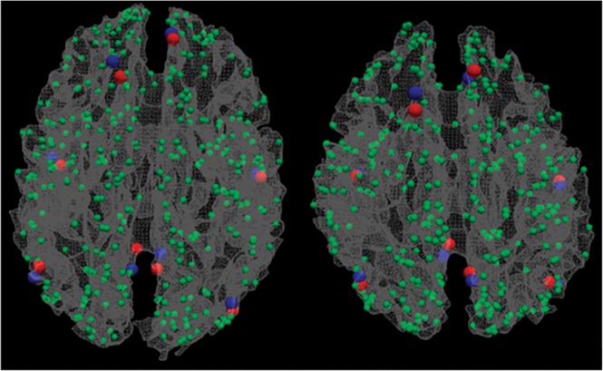
Two examples of mapping DICCCOL landmarks (blue) to fMRI benchmarks (red). The DMN is used here as an example.

Results

The Result section includes 3 parts as follows. Reproducibility and Predictability focuses on the reproducibility and predictability of the discovered DICCCOLs and an external independent structural validation using subcortical regions as benchmark landmarks. Functional Localizations of DICCCOLs focuses on functional colocalization and validations of these DTI-derived DICCCOLs via fMRI data. Comparison with Image Registration Algorithms compares the DICCCOL system with image registration algorithms.

Reproducibility and Predictability

The 358 DICCCOLs were identified via a data-driven whole brain search procedure (see Initialization and Overview of the DICCCOL Discovery Framework, Fiber Bundle Comparison Based on Trace-Maps, Optimization of Landmark Locations, Determination of Consistent DICCCOLs) in 10 randomly selected subjects from data set 2 (equally and randomly divided into 2 independent groups), as shown in Figure 5a. As an example, we randomly selected 5 DICCCOLs (5 enlarged color spheres in Fig. 5a) and plotted their emanating fibers in these 10 brains (Fig. 5b–f). It can be clearly seen that the fiber connection patterns of the same landmark in 10 brains are very consistent, suggesting that DICCCOLs represent common structural cortical architecture. Importantly, by visual inspection, all these 358 DICCCOLs have consistent fiber connection patterns in these 10 brains. For more details, the visualization of all these 358 landmarks is available online at http://dicccol.cs.uga.edu. In addition to visual evaluation, we quantitatively measured the differences of fiber shape patterns represented by the trace-maps (see Fiber Bundle Comparison Based on Trace-Maps) for each DICCCOL within and across 2 groups (Fig. 5l–n). The average trace-map distance is 2.19, 2.05, and 2.15 using equation (4). It is evident that the quantitative trace-map representations of fiber bundles for each DICCCOL has similar patterns within and across 2 separate groups, demonstrating the consistency of DICCCOL’s fiber connection patterns.

Figure 5.

(a) The 358 DICCCOLs. (b–f) DTI-derived fibers emanating from 5 landmarks (enlarged color bubbles in a) in 2 groups of 5 subjects (in 2 rows), respectively. (g–k) The predicted 5 landmarks in 2 groups of 5 subjects (in 2 rows) and their corresponding connection fibers. (l) Average trace-map distance for each landmark in the first group (rows in b–f); the color bar is on top of (o,p). (m) Average trace-map distance for each landmark in the second group (rows in b–f); (n) Average trace-map distance for each landmark across 2 groups in b–f; (o,p) Average trace-map distance for each landmark in the 2 predicted groups in g–k, respectively. (q) The decrease fraction of trace-map distance before and after optimization (the color bar on the top of q). The initialization was performed via a linear image warping algorithm.

In addition to the remarkable reproducibility of each DICCCOL in Figure 5b–f, the 358 DICCCOLs can be effectively and accurately predicted in a single separate brain with DTI data (other test cases in data set 2), as exemplified in Figure 5g–k. The landmark prediction will be evaluated by both fiber shape patterns (in this section) and functional locations (in Functional Localizations of DICCCOLs and Comparison with Image Registration Algorithms). Here, each landmark was predicted in 10 separate test brains (Fig. 5g–k) based on the template fiber bundles of corresponding landmarks (Fig. 5b–f). We can clearly see that the predicted landmarks have quite consistent fiber connection patterns in these test brains (Fig. 5g–k) as those in the template brains (Fig. 5b–f), indicating that the DICCCOLs are predictable across different brains. Quantitatively, the predicted landmarks have similar quantitative trace-map patterns as those in the template brains, as shown in Figure 5o,p. The average trace-map distance is 2.27 and 2.17. As a comparison, the predicted landmarks have much more consistent fiber trace-map patterns than the linearly registered ones via FSL FLIRT (Fig. 5q). The average decrease fraction of trace-map distance is 15.5%. We have applied the DICCCOL prediction framework in all the brains in data sets 1–4 and achieved very consistent results. These results support the DICCCOL as an effective quantitative representation of common structural cortical architecture that is reproducible and predicable across subjects and populations.

Also, we applied the DICCCOL prediction method in Prediction of DICCCOLs to localize the 358 DICCCOLs in all the brains in data sets 1–4. All the 358 predicted DICCCOLs in these populations are available online for visual examination: http://dicccol.cs.uga.edu. Figure 6a shows one example of a predicted DICCCOL landmark in one subject. In Figure 6a, the first 2 rows (n = 10) are models and last row (n = 5) is the predicted result in the new subject. The DICCCOL index shown in Figure 6a is #311. From the results in Figure 6a and online visualizations (http://dicccol.cs.uga.edu), we can see that: 1) given the DICCCOLs in the model brains, we can effectively predict their corresponding counterparts in a new brain with DTI data; 2) the patterns of fiber bundles of corresponding DICCCOLs in the predicted brains are consistent with those in the model brains. We have visually examined all the 358 predicted DICCCOLs in 4 different data sets (143 brains) and found the similar conclusion. These comprehensive results on 4 different data sets over 143 brains indicate that our DICCCOLs can potentially reveal the common structural connectivity patterns of the human brain.

Figure 6.

(a) An example of a predicted DICCCOL landmark (DICCCOL #311) in 5 separate subject brains. The first 2 rows (n = 10) are models, and last row (n = 5) is the predicted result in 5 brains. (b–e) Demonstration that fiber shape pattern represents structural connectivity pattern using subcortical regions as benchmark landmarks. (b) One DICCCOL landmark (blue sphere) and its fiber connections in 5 different brains. The 4 subcortical regions are represented by yellow, red, green, and cyan colors in d. The fibers connected to these subcortical regions are in the same colors. It is evident that this DICCCOL landmark has the same pattern of structural connectivity to these subcortical regions. (c) Another lateral view of the fiber connection patterns. (d) Color codes for cortical surface, landmark ROI, and subcortical regions. (e) The average distances of structural connectivity patterns for 175 DICCCOL landmarks that have strong fiber connections (over 50 fibers) to subcortical regions. Other DICCCOL landmarks are shown in green.

To verify that the DTI-derived fiber patterns of DICCCOLs discovered in Optimization of Landmark Locations and Determination of Consistent DICCCOLs faithfully represent structural connectivity patterns, we used subcortical regions, which are relatively consistent and reliable, as benchmark landmarks for measurement of consistency of DICCCOL’s structural connectivities (Zhu et al. 2011a). The subcortical regions were segmented via the FSL FIRST toolkit from MRI image (e.g., Fig. 6b–d) and then linearly warped to DTI image via FSL FLIRT. Our results demonstrate that 175 of the 358 DICCCOLs have strong connections (over 50 streamline fibers) to subcortical regions and all of them have quite consistent structural connectivities to subcortical regions. Specifically, we constructed a feature vector <V1, V2, V3, V4, V5, V6> to represent the connectivity pattern from cortical region to the intrahemisphere subcortical structures (amygdala, hippocampus, thalamus, caudate, putamen, and globus pallidus). For instance, if there is any fiber that connects the cortical region to a specified subcortical region, we set its corresponding item to one. Otherwise, it is set to zero. Then, we used the L-2 distance to measure group distance of the cortical–subcortical connectivity patterns, which are color coded in Figure 6e. The average L-2 distance for all these 175 DICCCOL landmarks over 10 subjects is 1.42, which is considered as quite low. This result suggests that consistent fiber shape patterns of DICCCOL landmarks indeed represent consistent structural connectivity patterns.

Functional Localizations of DICCCOLs

The major objective of performing functional localization of DICCCOLs in this section is to demonstrate that structural DICCCOL landmarks with consistent fiber shape patterns possess corresponding functional localizations. In total, we were able to identify 121 functional ROIs that were consistently activated from 9 brain networks (working memory, default mode, auditory, semantic decision making, emotion, empathy, fear, attention, and visual networks) based on the fMRI data sets in Data Acquisition and Preprocessing. More details of these 121 ROIs including coordinates in MNI_152 template space and BAs are summarized in Supplementary Table 2. To examine the functional colocalizations of 358 DICCCOLs, we mapped the 121 functionally labeled brain ROIs onto the DICCCOL map by the methods in Mapping fMRI-Derived Benchmarks to DICCCOLs. Surprisingly, 95 of the 358 DICCCOLs were consistently colocalized in one or more functional brain networks determined by fMRI data sets across different subjects and/or populations (see Fig. 7). Specifically, 76 of them are located adjacently to one functional network, 16 of them are located within 2 functional networks, and 3 of them are located inside 3 functional networks.

Figure 7.

Functional localizations of 95 DICCCOLs determined by 121 fMRI-derived functional regions. Specifically, 76 of them are located adjacently to one functional network, 16 of them are located within 2 functional networks, and 3 of them are located inside 3 functional networks. (a) Working memory network (data set 2). White spheres represent fMRI-derived benchmarks and yellow spheres represent corresponding DICCCOLs. The distances between centers of fMRI benchmarks and DICCCOLs are shown in the bottom panel, in which the horizontal axis indexes activations and the vertical axis is the distance in the unit of millimeter. Each bar represents the median (interface between the red and yellow bars), minimum and maximum value (2 ends of the white line), 25% (bottom of the red bar), and 75% (top of the yellow bar) of the distances for each fMRI activation peak. The average distance is 6.07 mm (b–i) results for default mode (data set 1), auditory (data set 4), semantic decision making (data set 1), emotion (data set 1), empathy (data set 1), fear (data set 1), attention (data set 3), visual networks (data set 4), respectively. In b–i, white spheres stand for fMRI benchmarks and other colors represent corresponding DICCCOLs. The average distances between centers of fMRI benchmarks and DICCCOLs in these networks are 5.50, 6.48, 6.25, 6.12, 6.41, 5.93, 5.94, and 7.59 mm, respectively.

To quantitatively evaluate the functional localization accuracy by the 95 DICCCOLs, we measured the Euclidean distance between the centers of each DICCCOL and each fMRI-derived landmark and reported the results in Figure 7. There are 9 subfigures corresponding to the 9 functional networks identified using fMRI data sets, that is, working memory (Fig. 7a), default mode (Fig. 7b), auditory (Fig. 7c), semantic decision making (Fig. 7d), emotion (Fig. 7e), empathy (Fig. 7f), fear (Fig. 7g), attention (Fig. 7h), and visual networks (Fig. 7i), respectively. In each subfigure, the fMRI-derived landmarks are highlighted by white spheres, while the corresponding DICCCOLs are highlighted in other colors. The distances (measured in millimeter) between the centers of fMRI landmarks and DICCCOLs are shown in the bottom panel, in which the horizontal axis indexes activations and the vertical axis is the distance in the unit of mm. Each bar represents the median (interface between the red and yellow bars), minimum and maximum value (2 ends of the white line), 25% (bottom of the red bar), and 75% (top of the yellow bar) of the distances for each fMRI activation peak. The average distances for the 9 functional networks are 6.07, 5.43, 6.48, 6.25, 6.12, 6.41, 5.93, 5.94, and 7.59 mm, respectively. On average, the distance is 6.25 mm. The results in Figure 7 demonstrate that the DICCCOLs are consistently colocalized with functional brain regions, and the DICCCOL map itself offers an effective and quantitative representation of common functional cortical architecture that is reproducible across subjects and populations.

It is notable that due to the limited number of subjects scanned in the task-based fMRI of the 8 networks, the dominant DICCCOLs within those task-based networks displayed in Figure 7 were acquired by using all the fMRI scans available in data sets 1–4. To study the reproducibility of the mapping between functional ROIs and the DICCCOL map, we used the DMN as a test bed, since R-fMRI data were available in 3 independent groups (i.e., healthy adolescents [N = 26], healthy adults [N = 53] and healthy elders [N = 23] from data set 4, see Data Acquisition and Preprocessing for details). These data sets have 102 subjects and cover a wide range of ages (see Supplementary Table 1 for demographics). In particular, the elders were scanned separately with 2 different sets of imaging parameters, which provides an ideal evaluation of the robustness of mapping functional ROIs onto DICCCOLs. Two examples of the study results are provided in Supplementary Figure 1, in which red spheres represent the predefined R-fMRI-derived benchmarks and the blue ones are the DICCCOL representations of these functional ROIs. Supplementary Figure 1a shows a cross-session comparison result for the same subject with 2 repeated scans, while Supplementary Figure 1b depicts the DICCCOL representations for 2 randomly selected subjects. As we can see from the figure, the DICCCOLs have a robust and effective representation of the ROIs in DMN across imaging scans and different subjects.

The quantitative evaluations applied on the 4 different subject groups are summarized in Table 2. There are 8 DMN ROIs identified (Identification of Functionally Relevant Landmarks via fMRI), corresponding to ROI#1∼ROI#8 respectively in Table 2. As we can see from the table, the dominant DICCCOLs for the 4 independent groups are strikingly the same, and the Euclidian distance from the dominant DICCCOLs to the benchmarks is consistently small across the 4 independent subject groups, averaged at 5.43 ± 2.59 mm. Besides, the 2 independent data sets from the elders (the first 2 panels in Table 2) have similar results in terms of the mean distance and variance. These results indicate that our DICCCOL representation of functional ROIs is accurate, robust, consistent, and reproducible in multiple multimodal fMRI and DTI data sets across populations.

Table 2.

Reproducibility study on DICCCOL representation of DMN ROIs for 4 subject groups

ROI	ROI1	ROI2	ROI3	ROI4	ROI5	ROI6	ROI7	ROI8
DICCCOL ID	326	76	144	45	298	79	155	72
Distance: mean	4.20	4.44	3.81	4.40	4.32	6.96	8.63	5.00
Distance: SD	2.16	3.23	1.82	2.03	2.39	3.07	3.24	3.58
DICCCOL ID	326	76	144	45	298	79	155	72
Distance: mean	5.11	4.13	4.90	5.06	5.22	5.74	6.38	6.32
Distance: SD	1.65	2.32	2.90	2.52	2.37	3.22	3.43	3.55
DICCCOL ID	326	76	144	45	298	79	155	72
Distance: mean	5.12	5.32	4.51	5.25	5.35	6.39	4.45	5.80
Distance: SD	2.41	2.99	2.25	2.36	2.47	3.17	1.57	2.89
DICCCOL ID	326	76	144	45	298	79	155	72
Distance: mean	5.40	6.42	4.83	6.11	6.27	7.48	5.77	4.84
Distance: SD	2.13	3.40	1.77	2.16	2.74	3.22	1.97	2.13

Note: Each color represents a data set. From top to bottom are elderly group (N = 23) in data set 4, the same elderly group with repeated R-fMRI scans in data set 4, adult group (N = 53) in data set 4, and adolescent group (N = 26) in data set 4. Distances are measured in millimeter.

Comparison with Image Registration Algorithms

In addition, we performed a comparison study on the functional localization accuracy by DICCCOL and FSL’s FLIRT image registration (Jenkinson and Smith 2001) that was performed on MRI images. Here, the fMRI-derived functional landmarks were used as the benchmark data for comparison. The image registration error was defined as the distance between the linearly transformed fMRI peaks from individual subjects in the MNI atlas space to the centers of these multiple subjects’ transformed fMRI-derived peaks. Here, we used the individualized activation peaks in 9 networks as the benchmarks. The DICCCOL error is defined as the distance between the dominant DICCCOL and benchmark. The comparisons for the 9 brain networks are summarized in Table 3. Overall, the average of the distance by our DICCCOL over 9 networks is 6.25 mm. The average FSL FLIRT linear image registration error is 8.70 mm, which is 39% larger than that of DICCCOL. For statistical comparisons of our DICCCOL method and the FSL FLIRT, the P values were also calculated. As summarized in Table 3, most networks have P value < 0.05. These comparison results show that DICCCOL has superior localization accuracy compared with the FSL FLIRT image registration strategy (Jenkinson and Smith 2001).

Table 3.

Comparisons of functional localization accuracies by DICCCOL and FSL FLIRT

	WM	DMN	Visual	Auditory	Emotion	Attention	Fear	SDM	Empathy
DICCCOL	6.07	5.43	7.59	7.48	6.12	5.94	5.93	6.25	6.41
FLIRT	9.13	6.92	15.21	14.34	6.86	7.57	7.41	8.25	7.20
P value	1.30 × 10−05	1.52 × 10−03	3.57 × 10−06	5.35 × 10−05	2.25 × 10−01	6.65 × 10−08	4.62 × 10−02	2.34 × 10−03	2.58 × 10−01

Besides, we performed a comparison between our DICCCOL method and other 3 different non-linear image registration algorithms, including FNIRT (Andersson et al. 2008), ANTS (Avants et al. 2008), and HAMMER (Shen and Davatzikos 2002), using the fMRI-derived working memory ROIs as benchmarks. The average localization errors by the 5 methods (FLIRT, FNIRT, ANTS, HAMMER, and DICCCOL) are 8.17, 8.35, 8.19, 8.15, and 6.08 mm, respectively. The comparison results in Supplementary Figure 2 indicate that these image registration algorithms have similar performances in terms of the registration error from the benchmarks, and no one is superior to others for all working memory functional ROIs. Importantly, the result also shows that our DICCCOL method has superior localization accuracy than these 3 nonlinear image registration algorithms for functional ROI localization. Notably, these compared image registration algorithms were originally designed for anatomical alignments but not specifically for functional ROI localization. If these image registration algorithms take the advantage of multimodal data in the future, their performances for functional ROI localization could be substantially better than what was reported here.

Application

Human connectomes constructed via neuroimaging data offer a complete description of the macroscale structural connectivity within the brain (Hagmann et al. 2010; Kennedy 2010; Van Dijk et al. 2010; Williams 2010). Given the intrinsically established correspondences across individuals, the 358 common DICCCOLs provide natural structural substrates for assessments of large-scale structural and functional connectivities within the connectomes. Our general hypothesis is that the structural and functional connectomes constructed via the DICCCOLs have close relationships and are relatively consistent across age populations. After predicting the DICCCOL map in 3 age groups of adolescents (22 subjects), adults (44 subjects), and elders (23 subjects), we constructed large-scale structural (by streamline fiber numbers, Zhang et al. 2010 and Yuan et al. 2011) and functional (Pearson correlation between representative fMRI signals after PCA transforms, Li et al. 2010) connectivities of individuals in 3 age groups. It is noted that our purpose is to map the structural fiber pathways among DICCCOLs in healthy brains and we assume that there is no significant difference in diffusivity along these pathways in normal brains, which is the case in our experimental results. Therefore, we used the number of fiber tracts as the connection strength. Figure 8a–c and Figure 8d–f show their structural and resting-state functional connectomes, respectively. When comparing the structural connectomes across the 3 age groups, it is inspiring that the structural connectomes are consistent across the 3 age groups. Specifically, as shown in Figure 8j, there are around 74–80% common edges across 2 age groups, and in particular, there are approximately 67% common edges across all 3 age groups.

Figure 8.

Structural and functional (resting-state) human brain connectomes. (a–c) Structural connectomes in adolescent (n = 22), adult (n = 44), and elderly (n = 23) groups. Each structural connectome is obtained by the averaged structural connectivity between each pair of DICCCOLs in each age group. The color bar at the bottom of c encodes the number of streamline fibers (from 10 to 150). (d–f) Functional connectomes in the 3 age groups. Each functional connectome is obtained by the averaged functional connectivity between each pair of DICCCOLs in each age group. The color bar at the bottom of f encodes the average functional connectivity (from 0.45 to 0.8). (g–i) The percentages of functional connections in d–f that are coincident with direct and indirect (up to 4 path lengths) structural connections, for 3 age groups, respectively. The horizontal axis represents the threshold used to select the functional connection edges and the number of selected functional edges in the connectivity matrix, and the vertical axis is the ratio of structural connections that are coincident with functional connections. Path length 1 (red curve) means direct structural connection between 2 DICCCOLs, while path length 2 (green curve), 3 (blue curve), and 4 (pink curve) represent 2–4 structural connection edges between 2 DICOOOLs. In particular, the black dotted curves in g shows that around 80% of functional connections in d in the adolescent group have direct or indirect structural connections. We can see similar black dotted curves in h and i for the adult and elder groups. (j) Percentages of common structural connectome edges between 2 groups and across 3 groups. The horizontal axis stands for the thresholds used to select the structural connection edges and the numbers of selected edges in the connectivity matrix, and the vertical axis is the ratio of common structural edges between 2 or 3 structural connectivity matrices. (k) Percentages of common functional connectome edges between 2 groups and across 3 groups. The horizontal axis represents the thresholds used to select the functional connection edges and the numbers of totally selected edges in the functional connectivity matrix, and the vertical axis is the ratio of common functional edges between 2 or 3 functional connectivity matrices.

When comparing the resting-state functional connectomes across the 3 age groups, it is also interesting that the resting-state functional connectomes are also reasonably consistent across these 3 age groups. Specifically, as shown in Figure 8k, there are around 55–70% common edges across 2 age groups, despite more functional connections in the adolescent group (Fig. 8d–f). In particular, there are approximately 47% common edges across all 3 age groups. We further examined the relationship between structural and functional connectomes. As shown in Figure 8g–i, for each age group, approximately 78% of the common functional connections (Fig. 8g–i) have direct or indirect structural common connections, suggesting the structural underpinnings of functional connectivities. These results demonstrate that the DICCCOL representation of common cortical architecture reveals common structural and functional connectomes and their close relationship. According to the above results, we demonstrated that there is a deep-rooted regularity of cortical architectures among healthy human brains (despite normal variation due to age differences). Furthermore, the DICCCOL map can indeed represent common cortical architecture and reveal common structural and functional connectomes, as well as their close relationships across human brains.

To compare the DICCCOL-based structural connectivity mapping with that by the MNI atlas-based method, Supplementary Figure 3a,b show the mapped structural connectivities obtained by these 2 methods, respectively. As demonstrated in Supplementary Figure 3, the major advantage of using DICCCOL for structural connectivity construction is that this method offers finer granularity, better functional homogeneity, more accurate functional localization, and automatically established cross-subjects correspondence. For instance, a single ROI at the gyrus scale in Supplementary Figure 3b was represented by multiple DICCCOL ROIs with finer granularity and more functional homogeneity. Meanwhile, the overall structural connectivity patterns among the gyrus-scale ROIs in Supplementary Figure 3b were also well preserved in the DICCCOL-scale connectivity map in Supplementary Figure 3a.

Discussion and Conclusion

As summarized in Figure 9, our data-driven discovery approach has identified 358 DICCCOLs that are consistent and reproducible across over 143 brains based on DTI data. Extensive studies have shown that these 358 landmarks can be accurately predicted across different subjects and populations. Our work has demonstrated that there is deep-rooted regularity in the structural architecture of the cerebral cortex, which has been jointly and spontaneously encoded by the DICCCOL map. The DICCCOL map has been evaluated by 4 independent multimodal fMRI and DTI data sets which consisted of 143 subjects covering different age groups, that is, adolescent, adult, and elderly. In total, 121 consistent and stable functional ROIs derived from 8 task-based fMRI network (auditory, attention, emotion, empathy, fear, semantic decision making, visual, and working memory networks) and one R-fMRI network (DMN), shown in Figure 9b–j, were used to functionally label the predicted DICCCOLs for individuals. Our extensive experimental results demonstrated that the DICCCOL representation of functional ROIs is accurate, robust, consistent, and reproducible in multiple multimodal fMRI and DTI data sets. The advantage of the DICCCOL-based brain reference system in comparison with brain image registration methods (see Comparison with Image Registration Algorithms) has been demonstrated by validation studies using fMRI-derived brain networks. With the universal DICCCOL brain reference system, different measurements of the structural and functional properties of the brain, for example, morphological measurements derived from structural MRI data and functional measurements derived from fMRI data, can be reported, integrated, and compared within the DICCCOL reference system. For instance, we can report fMRI-derived activated regions by their corresponding closest DICCCOL IDs, instead of their stereotaxic coordinates in relation to the Talairach or MNI coordinate system. This principled and universal DICCCOL brain reference system could be an effective solution to the widely recognized problem of “blobology” in fMRI research (Poldrack 2011).

Figure 9.

Summary of our approach and results. Spheres in orange (total 6), red (total 8), brown (total 9), pink (total 8), blue (total 27), yellow (total 14), cyan (total 14), purple (total 16), and black-red (total 19) colors stand for landmarks in empathy, default mode, visual, auditory, attention, working memory, fear, emotion, and semantic decision making networks that are identified from fMRI data sets. The green spheres (totally 263) stand for landmarks that are not functionally labeled yet. The DICCCOLs serve as structural substrates to represent the common human brain architecture. For instance, 9 different functionally specialized brain networks (b–j) identified from different fMRI data sets are integrated into the same universal brain reference system (a) via DICCCOL. Then, the functionally labeled DICCCOLs in the universal space can be predicted in each individual brain with DTI data such that the DICCCOLs and their functional identities can be readily transferred to a local coordinate system (k).

In a broader sense, the DICCCOL map provides a general platform to aggregate and integrate functional networks from different multimodal DTI and fMRI data sets to the universal DICCCOL map, the sum of which can then be transferred to a new separate individual or population via DTI data. For instance, the functional labeling of a portion of the DICCCOLs in an individual data set, for example, in Figure 9b–j, can be readily transferred to the universal template space (Fig. 9a) and then be propagated to other individual brains, as shown in Figure 9k. In this way, specific functional localizations on the DICCCOL map achieved in one multimodal fMRI and DTI data set (e.g., Fig. 9b–j) can contribute to the same functional localization problem in other brains, once DTI data, on which the DICCCOL map prediction can be accurately performed, is available (e.g., Fig. 9k). This common DICCCOL platform offers an alternative approach and can be complementary to current methods (e.g., Van Horn et al. 2004; Derrfuss and Mar 2009), such that contributions from different laboratory can be effectively integrated and compared.

The powerfulness of the DICCCOL map and its potential impact on the brain science has been exemplified by its application to the discoveries of structural and functional human brain connectomes (Biswal et al. 2010; Hagmann et al. 2010; Kennedy 2010; Van Dijk et al. 2010; Williams 2010) in various age populations. The idea of connectome was proposed recently (Hagmann et al. 2005) to represent the notion that the brain is a large network composed of neural connections (edges) and neural units (nodes). It has attracted significant interest (Biswal et al. 2010; Hagmann et al. 2010; Van Dijk et al. 2010) and efforts in an attempt to map the nodes and edges in the brain at both individual and population level. Quantitative mapping of the human brain connectome offers a unique and exciting opportunity to understand the fundamental cortical architecture. When mapping human brain connectomes, the network nodes ROIs provide the structural substrates for connectivity mapping. Thus, the determination of accurate and reliable ROIs in different brains is critically important in human brain connectome mapping (Liu 2011). In this paper, the 358 common, reliable, reproducible, and accurate DICCCOLs provide a natural choice of ROIs for human brain connectome mapping. Because the 358 DICCCOLs were discovered and defined by maximizing the group-wise consistency of ROIs’ white matter fiber connectivity patterns across a group of subjects, the uncertainties and variations in the localizations of corresponding ROIs across different brains and populations are substantially reduced. This principled approach of ROI determination significantly facilitates the construction of reliable and reproducible human brain connectomes. Importantly, these 358 DTI-derived DICCCOLs turn out to be well colocalized with functional brain regions determined by fMRI data. Hence, the human brain connectomes constructed based on the 358 DICCCOL ROIs reveal that there is deep-rooted regularity of connectomes across human brains of different ages and there is close relationship between structural and functional connectomes.

Notably, there are several limitations in the current study that should be addressed in future work. 1) In current stage, only 358 DICCCOLs were discovered of the 2056 initialized landmark candidates. This might reflect a combination of factors including intersubject variability, the limited resolution of DTI data, and the limitation of our DICCCOL discovery procedure. In the future, more consistent DICCCOLs could be possibly discovered via high-quality data and improved computational approaches. For instance, one of our ongoing works is to further improve the resolution of DICCCOLs via high-angular resolution diffusion imaging data. Another possible improvement is to refine our optimization procedure. For example, instead of using trace-map distance as main metric, in the future, we can introduce more informative constraints such as anatomical and functional homogeneity by which we could discover more DICCCOLs. 2) We hypothesize that there exists huge potential for the functional mapping of the DICCCOLs since the fMRI tasks used in this paper were not originally designed for this DICCCOL study. Although their applications in the independent validation of functional correspondences of DICCCOLs are meaningful and helpful, in the future, a systematic design of task paradigms should be considered to comprehensively validate the functional identities of DICCCOLs. 3) This work has demonstrated the close relationship between the structure and function of the brain. However, only the white matter fiber connectivity patterns were considered in this work, and other potentially important anatomic information such as cortical folding patterns, cortical thickness, and MRI image intensity features was not used. It will be interesting to study the correlations between those anatomic features and DICCCOLs and investigate how the combination of different structural features would influence the functional ROI prediction. 4) It should be noted that, in this paper, the DICCCOLs focuses on representing the common cortical architectures. They can possibly serve as the foundation for additional approaches to be developed and validated in the future to represent the normal intersubject variability of cortical architectures.

In the future, the DICCCOL map can be applied for the elucidations of possible large-scale connectivity alterations in brain diseases. Tremendous efforts have been made to examine the hypothesized connectivity alterations in brain diseases, for example, aberrant default mode functional connectivity has been found in schizophrenia (SZ), mild cognitive impairment (MCI) and post-traumatic stress disorder (PTSD) (e.g., Garrity et al. 2007; Bai et al. 2008; Bluhm et al. 2009). In most studies, connectivity alterations were only evaluated in one or a few small networks in the human brain, for example, based on the brain regions detected in a specific task-based fMRI (Atri et al. 2011; Yu et al. 2011) or resting-state fMRI (Greicius et al. 2004; Sorg et al. 2007; Greicius 2008) scan. Due to the lack of dense brain landmarks with correspondences across different brains and the unavailability of extensive task-based fMRI data (i.e., it is impractical for children or elder patients to perform extensive tasks during neuroimaging scans), it has been very challenging to map large-scale structural and functional connectivities in brain diseases, even though a variety of brain disease are hypothesized to exhibit large-scale connectivity alterations (Supekar et al. 2008; Dickerson and Sperling 2009; Seeley et al. 2009; Suvak and Barrett 2011). In the future, we plan to apply the 358 DICCCOLs to construct large-scale networks for the elucidation of widespread structural/functional connectivity alterations for brain diseases such as SZ, MCI, and PTSD.

In summary, the DICCCOLs representation of common cortical architecture offers a principled approach and a generic platform to share, exchange, integrate, and compare neuroimaging data sets across laboratories, and thus we predict that public release of our DICCCOL models (http://dicccol.cs.uga.edu) and the release of DICCCOL prediction tools (http://dicccol.cs.uga.edu/dicccol.tar.gz) could stimulate and enable many collaborative efforts in brain sciences, as well as accelerating the pace of data-driven discovery brain imaging science. For instance, different laboratory can contribute their multimodal DTI and fMRI data sets to further perform functional labeling and validation of those 358 DICCCOLs in healthy brains and tailor them toward different brain disease populations.

Supplementary Material

Supplementary material can be found at: http://www.cercor.oxfordjournals.org/

Funding

T.L. was supported by the NIH K01 EB 006878, NIH R01 HL087923-03S2, and The University of Georgia start-up research funding. L.G., G.L. were supported by the NWPU Foundation for Fundamental Research. K.L., T.Z., and D.Z. were supported by the China Government Scholarship. L.L. was supported by The National Natural Science Foundation of China (30830046) and The National 973 Program of China (2009 CB918303). L.W. was supported by the Paul B. Beeson Career Developmental Awards (K23-AG028982) and National Alliance for Research in Schizophrenia and Depression Young Investigator Award.

References

- Andersson J, Smith S, Jenkinson M. 14th Annual Meeting of the Organisation for Human Brain Mapping; 2008 June 15--19; Melbourne, Australia: Organization for Human Brain Mapping. 2008. FNIRT—FMRIB’s non-linear image registration tool; p. 496. [Google Scholar]
- Asman AJ, Landman BA. Characterizing spatially varying performance to improve multi-atlas multi-label segmentation. Inf Process Med Imaging. 2011;6801:85–96. doi: 10.1007/978-3-642-22092-0_8. [DOI] [PMC free article] [PubMed] [Google Scholar]
- Atri A, O'Brien JL, Sreenivasan A, Rastegar S, Salisbury S, DeLuca AN, O'Keefe KM, LaViolette PS, Rentz DM, Locascio JJ, et al. Test-retest reliability of memory task functional magnetic resonance imaging in Alzheimer disease clinical trials. Arch Neurol. 2011;68(5):599–606. doi: 10.1001/archneurol.2011.94. [DOI] [PMC free article] [PubMed] [Google Scholar]
- Avants BB, Epstein CL, Grossman M, Gee JC. Symmetric diffeomorphic image registration with cross-correlation: evaluating automated labeling of elderly and neurodegenerative brain. Med Image Anal. 2008;12:26–41. doi: 10.1016/j.media.2007.06.004. [DOI] [PMC free article] [PubMed] [Google Scholar]
- Bai F, Zhang Z, Yu H, Shi Y, Yuan Y, Zhu W, Zhang X, Qian Y. Default-mode network activity distinguishes amnestic type mild cognitive impairment from healthy aging: a combined structural and resting-state functional MRI study. Neurosci Lett. 2008;438:111–115. doi: 10.1016/j.neulet.2008.04.021. [DOI] [PubMed] [Google Scholar]
- Bajcsy R, Lieberson R, Reivich M. A computerized system for the elastic matching of deformed radiographic images to idealized atlas images. J Comput Assist Tomogr. 1983;7(4):618–625. doi: 10.1097/00004728-198308000-00008. [DOI] [PubMed] [Google Scholar]
- Behrens JBH, Robson TEJ, Drobnjak MD, Rushworth I, Brady MFS, Smith JM, Higham SM, Matthews DJ. Changes in connectivity profiles define functionally distinct regions in human medial frontal cortex. Proc Natl Acad Sci U S A. 2004;101:13335–13340. doi: 10.1073/pnas.0403743101. [DOI] [PMC free article] [PubMed] [Google Scholar]
- Biswal BB, Mennes M, Zuo XN, Gohel S, Kelly C, Smith SM, Beckmann CF, Adelstein JS, Buckner RL, Colcombe S, et al. Toward discovery science of human brain function. Proc Natl Acad Sci U S A. 2010;107:4734–4739. doi: 10.1073/pnas.0911855107. [DOI] [PMC free article] [PubMed] [Google Scholar]
- Bluhm RL, Williamson PC, Osuch EA, Frewen PA, Stevens TK, Boksman K, Neufeld RWJ, Théberge J, Lanius RA. Alterations in default network connectivity in posttraumatic stress disorder related to early-life trauma. J Psychiatry Neurosci. 2009;34(3):187–194. [PMC free article] [PubMed] [Google Scholar]
- Brodmann K. Vergleichende Lokalisationslehre der Großhirnrinde in ihren Prinzipien dargestellt auf Grund des Zellenbaues. Leipzig: Verlag von Johann Ambrosius Barth. 1909. [Google Scholar]
- Damoiseaux JS, Rombouts SA, Barkhof F, Scheltens P, Stam CJ, Smith SM, Beckmann CF. Consistent resting-state networks across healthy subjects. Proc Natl Acad Sci U S A. 2006;103(37):13848–13853. doi: 10.1073/pnas.0601417103. [DOI] [PMC free article] [PubMed] [Google Scholar]
- De Luca M, Beckmann CF, De Stefano N, Matthews PM, Smith SM. fMRI resting state networks define distinct modes of long-distance interactions in the human brain. Neuroimage. 2006;29(4):1359–1367. doi: 10.1016/j.neuroimage.2005.08.035. [DOI] [PubMed] [Google Scholar]
- Derrfuss J, Mar RA. Lost in localization: the need for a universal coordinate database. Neuroimage. 2009;48(1):1–7. doi: 10.1016/j.neuroimage.2009.01.053. [DOI] [PubMed] [Google Scholar]
- Dickerson BC, Sperling RA. Large-scale functional brain network abnormalities in Alzheimer's disease: insights from functional neuroimaging. Behav Neurol. 2009;21(1):63–75. doi: 10.3233/BEN-2009-0227. [DOI] [PMC free article] [PubMed] [Google Scholar]
- Faraco CC, Unsworth N, Langley J, Terry D, Li K, Zhang D, Liu T, Miller LS. Complex span tasks and hippocampal recruitment during working memory. Neuroimage. 2011;55(2):773–787. doi: 10.1016/j.neuroimage.2010.12.033. [DOI] [PubMed] [Google Scholar]
- Fischl B, Salat DH, Busa E, Albert M. Whole brain segmentation: automated labeling of neuroanatomical structures in the human brain. Neuron. 2002;33(3):341–355. doi: 10.1016/s0896-6273(02)00569-x. [DOI] [PubMed] [Google Scholar]
- Fox MD, Raichle ME. Spontaneous fluctuations in brain activity observed with functional magnetic resonance imaging. Nat Rev Neurosci. 2007;8:700–711. doi: 10.1038/nrn2201. [DOI] [PubMed] [Google Scholar]
- Garrity AG, Pearlson GD, McKiernan K, Lloyd D, Kiehl KA, Calhoun VD. Aberrant “default mode” functional connectivity in schizophrenia. Am J Psychiatry. 2007;164(7):1123. doi: 10.1176/ajp.2007.164.3.450. [DOI] [PubMed] [Google Scholar]
- Gerig G, Gouttard S, Corouge I. Analysis of brain white matter via fiber tract modeling. IEEE Eng Med Biol Soc. 2004;2:4421–4424. doi: 10.1109/IEMBS.2004.1404229. [DOI] [PubMed] [Google Scholar]
- Greicius M. Resting-state functional connectivity in neuropsychiatric disorders. Curr Opin Neurol. 2008;21(4):424–430. doi: 10.1097/WCO.0b013e328306f2c5. [DOI] [PubMed] [Google Scholar]
- Greicius MD, Srivastava G, Reiss AL, Menon V. Default-mode network activity distinguishes Alzheimer's disease from healthy aging: evidence from functional MRI. Proc Natl Acad Sci U S A. 2004;101(13):4637–4642. doi: 10.1073/pnas.0308627101. [DOI] [PMC free article] [PubMed] [Google Scholar]
- Hagmann P, Cammoun L, Gigandet X, Gerhard S, Grant PE, Wedeen V, Meuli R, Thiran JP, Honey CJ, Sporns O. MR connectomics: principles and challenges. J Neurosci Methods. 2010;194:34–45. doi: 10.1016/j.jneumeth.2010.01.014. [DOI] [PubMed] [Google Scholar]
- Honey CJ, Sporns O, Cammoun L, Gigandet X, Thiran JP, Meuli R, Hagmann P. Predicting human resting-state functional connectivity from structural connectivity. Proc Natl Acad Sci U S A. 2009;106(6):2035–2040. doi: 10.1073/pnas.0811168106. [DOI] [PMC free article] [PubMed] [Google Scholar]
- Jbabdi S, Woolrich MW, Behrens TEJ. Multiple-subjects connectivity-based parcellation using hierarchical Dirichlet process mixture models. Neuroimage. 2009;44:373–384. doi: 10.1016/j.neuroimage.2008.08.044. [DOI] [PubMed] [Google Scholar]
- Jenkinson M, Smith SM. A global optimisation method for robust affine registration of brain images. Med Image Anal. 2001;5(2):143–156. doi: 10.1016/s1361-8415(01)00036-6. [DOI] [PubMed] [Google Scholar]
- Jia H, Wu G, Wang Q, Shen D. ABSORB: atlas building by self-organized registration and bundling. Neuroimage. 2010;51(3):1057–1070. doi: 10.1016/j.neuroimage.2010.03.010. [DOI] [PMC free article] [PubMed] [Google Scholar]
- Kennedy DN. Making connections in the connectome era. Neuroinformatics. 2010;8(2):61–62. doi: 10.1007/s12021-010-9070-1. [DOI] [PubMed] [Google Scholar]
- Li K, Guo L, Faraco C, Zhu D, Deng D, Zhang T, Jiang X, Zhang D, Chen H, Hu H, et al. Individualized ROI optimization via maximization of group-wise consistency of structural and functional profiles. Adv Neural Inf Process Syst. 2010;23:1369–1377. [Google Scholar]
- Liu T. A few thoughts on brain ROIs, brain imaging and behavior. 2011 doi: 10.1007/s11682-011-9123-6. doi:10.1007/s11682-011-9123-6. [DOI] [PMC free article] [PubMed] [Google Scholar]
- Liu T, Shen D, Davatzikos C. Deformable registration of cortical structures via hybrid volumetric and surface warping. Neuroimage. 2004;22(4):1790–1801. doi: 10.1016/j.neuroimage.2004.04.020. [DOI] [PubMed] [Google Scholar]
- Logothetis NK. What we can do and what we cannot do with fMRI. Nature. 2008;453:869–878. doi: 10.1038/nature06976. [DOI] [PubMed] [Google Scholar]
- Maddah M, Mewes AUJ, Haker S, Grimson WEL, Warfield SK. Automated atlas-based clustering of white matter fiber tracts form DTMRI. Med Image Comput Comput Assist Interv. 2005;8:188–195. doi: 10.1007/11566465_24. [DOI] [PubMed] [Google Scholar]
- Mori S. Principles of diffusion tensor imaging and its applications to basic neuroscience research. Neuron. 2006;51(5):527–539. doi: 10.1016/j.neuron.2006.08.012. [DOI] [PubMed] [Google Scholar]
- O'Donnell LJ, Kubicki M, Shenton ME, Dreusicke MH, Grimson WE, Westin CF. A method for clustering white matter fiber tracts. Am J Neuroradiol. 2006;27:1032–1036. [PMC free article] [PubMed] [Google Scholar]
- Passingham RE, Stephan KE, Kotter R. The anatomical basis of functional localization in the cortex. Nat Rev Neurosci. 2002;3(8):606–616. doi: 10.1038/nrn893. [DOI] [PubMed] [Google Scholar]
- Poldrack RA. The future of fMRI in cognitive neuroscience. Neuroimage. 2011 doi: 10.1016/j.neuroimage.2011.08.007. doi:10.1016/j.neuroimage.2011.08.007. [DOI] [PMC free article] [PubMed] [Google Scholar]
- Seeley WW, Crawford RK, Zhou J, Miller BL, Greicius MD. Neurodegenerative diseases target large-scale human brain networks. Neuron. 2009;62(1):42–52. doi: 10.1016/j.neuron.2009.03.024. [DOI] [PMC free article] [PubMed] [Google Scholar]
- Shen D, Davatzikos C. HAMMER: hierarchical attribute matching mechanism for elastic registration. IEEE Trans Med Imaging. 2002;21(11):1421–1439. doi: 10.1109/TMI.2002.803111. [DOI] [PubMed] [Google Scholar]
- Sorg C, Riedl V, Mühlau M, Calhoun VD, Eichele T, Läer L, Drzezga A, Förstl H, Kurz A, Zimmer C, et al. Selective changes of resting-state networks in individuals at risk for Alzheimer's disease. Proc Natl Acad Sci U S A. 2007;104(47):18760–18765. doi: 10.1073/pnas.0708803104. [DOI] [PMC free article] [PubMed] [Google Scholar]
- Supekar K, Menon V, Rubin D, Musen M, Greicius MD. Network analysis of intrinsic functional brain connectivity in Alzheimer's disease. PLoS Comput Biol. 2008;4(6):e1000100. doi: 10.1371/journal.pcbi.1000100. [DOI] [PMC free article] [PubMed] [Google Scholar]
- Suvak MK, Barrett LF. Considering PTSD from the perspective of brain processes: a psychological construction approach. J Trauma Stress. 2011;24(1):3–24. doi: 10.1002/jts.20618. [DOI] [PMC free article] [PubMed] [Google Scholar]
- Thompson PM, Toga AW. A surface-based technique for 1336 warping 3-dimensional images of the brain. IEEE Trans Med Imaging. 1996;15(4):1–16. doi: 10.1109/42.511745. [DOI] [PubMed] [Google Scholar]
- van den Heuvel VM, Mandl R, Hulshoff Pol H. Normalized cut group clustering of resting-state FMRI data. PLoS One. 2008;3(4):e2001. doi: 10.1371/journal.pone.0002001. [DOI] [PMC free article] [PubMed] [Google Scholar]
- Van Dijk KR, Hedden T, Venkataraman A, Evans KC, Lazar SW, Buckner RL. Intrinsic functional connectivity as a tool for human connectomics: theory, properties, and optimization. J Neurophysiol. 2010;103(1):297–321. doi: 10.1152/jn.00783.2009. [DOI] [PMC free article] [PubMed] [Google Scholar]
- Van Essen DC, Dierker DL. Surface-based and probabilistic atlases of primate cerebral cortex. Neuron. 2007;56(2):209–225. doi: 10.1016/j.neuron.2007.10.015. [DOI] [PubMed] [Google Scholar]
- Van Horn JD, Grafton ST, Rockmore D, Gazzaniga MS. Sharing neuroimaging studies of human cognition. Nat Neurosci. 2004;7:473–481. doi: 10.1038/nn1231. [DOI] [PubMed] [Google Scholar]
- Williams R. The human connectome: just another 'ome. Lancet Neurol. 2010;9(3):238–239. doi: 10.1016/S1474-4422(10)70046-6. [DOI] [PubMed] [Google Scholar]
- Yap P, Gilmore JH, Lin W, Shen D. POPTRACT: population-based tractography. IEEE Trans Med Imaging. 2011;30:1829–1840. doi: 10.1109/TMI.2011.2154385. [DOI] [PMC free article] [PubMed] [Google Scholar]
- Yu Q, Sui J, Rachakonda S, He H, Pearlson G, Calhoun VD. Altered small-world brain networks in temporal lobe in patients with schizophrenia performing an auditory oddball task. Front Syst Neurosci. 2011;8:5–7. doi: 10.3389/fnsys.2011.00007. [DOI] [PMC free article] [PubMed] [Google Scholar]
- Yuan Y, Guo L, Lv P, Hu X, Zhang D, Han J, Xie L, Liu T. Assessing Graph models for description of brain networks. IEEE Int Symp Biomed Imaging. 2011:827–831. [Google Scholar]
- Zhang D, Guo L, Li G, Nie J, Jiang X, Deng F, Li K, Zhu D, Zhao Q, Liu T. Automatic cortical surface parcellation based on fiber density information. Int Symp Biomed Imaging. 2010:1133–1136. [Google Scholar]
- Zhang P, Cootes TF. Automatic part selection for groupwise registration. Inf Process Med Imaging. 2011;6801:85–96. doi: 10.1007/978-3-642-22092-0_52. [DOI] [PubMed] [Google Scholar]
- Zhang T, Guo L, Li K, Jing C, Hu X, Cui G, Li L, Liu T. Predicting functional cortical ROIs via DTI-derived fiber shape models. Cereb Cortex. 2011 doi: 10.1093/cercor/bhr152. doi:10.1093/cercor/bhr152. [DOI] [PMC free article] [PubMed] [Google Scholar]
- Zhu D, Li K, Faraco C, Deng F, Zhang D, Jiang X, Chen H, Guo L, Miller S, Liu T. Discovering dense and consistent landmarks in the brain. Inf Process Med Imaging. 2011a;22:97–110. doi: 10.1007/978-3-642-22092-0_9. [DOI] [PubMed] [Google Scholar]
- Zhu D, Li K, Faraco C, Deng F, Zhang D, Jiang X, Chen H, Guo L, Miller L, Liu T. Optimization of functional brain ROIs via Maximization of consistency of structural connectivity profiles. Neuroimage. 2011b;59(2):1382–1393. doi: 10.1016/j.neuroimage.2011.08.037. [DOI] [PMC free article] [PubMed] [Google Scholar]
- Zilles K, Amunts K. Centenary of Brodmann’s map—conception and fate. Nat Rev Neurosci. 2009;11:139. doi: 10.1038/nrn2776. [DOI] [PubMed] [Google Scholar]
Associated Data
This section collects any data citations, data availability statements, or supplementary materials included in this article.