Measuring Relative Timings of Brain Activities Using FMRI

Abstract

Functional MRI (fMRI) has previously been shown to be able to measure hundreds of milliseconds differences in timings of activities in different brain regions, even though the underlying blood oxygenation level-dependent (BOLD) response is delayed and dispersed on the order of seconds. This capability may contribute towards the study of communication within the brain by assessing the temporal sequences of various brain processes (mental chronometry). The practical limit of fMRI for detecting the relative timings of brain activities is not known. We aimed to detect fine differences in the timings of brain activities beyond those previously measured from fMRI data in human subjects. We introduced known delays between the onsets of visual stimuli in a controlled, sparse event-related design and investigated if the temporal shifts in the corresponding average BOLD signals were detectable. To maximize sensitivity, we used high spatial and temporal resolution fMRI at ultrahigh field (7 Tesla), in conjunction with a novel data-driven technique for voxel selection using graph-based visualizations of self-organizing maps and Granger causality to measure relative timing. This approach detected timing differences as small as 28 ms in visual cortex in individual subjects. For signal extraction, the self-organizing map approach outperformed other common techniques including independent component analysis, voxelwise univariate linear regression analysis and a separate localizer scan. For relative timing measurement, Granger causality outperformed time-to-peak calculations derived from an inverse logit curve fit. We conclude that high-resolution imaging at ultrahigh field, signal extraction via self-organizing map, and appropriate use of Granger causality permit the detection of small timing differences in fMRI data, despite the intrinsically slow hemodynamic response.

Introduction

Correct measurements of the timings of brain activities are critical for more fully understanding the neural dynamics of brain processes. Functional MRI (fMRI) has shown to be able to measure timing differences of the order of hundreds of milliseconds in brain activations despite its generally poor temporal resolution. The ability to detect short timing differences with fMRI may help to decode the sequential patterns of brain activity (mental chronometry), providing further insights into the nature of brain function during complex cognitive tasks.

FMRI is an indirect measure of neuronal activity. It does not measure neural, electrical or chemical changes but instead detects hemodynamic effects using blood oxygenation level-dependent (BOLD) responses that are delayed and dispersed in time. The hemodynamic response to brief neuronal activity typically takes 5–8 s to peak and 15–30 s to return to baseline, depending on the neurovascular coupling that may vary across brain regions. This precludes accurate measurement of the absolute timing of neuronal activity. However, hemodynamics can generally be assumed to be consistent and deterministic in time at a given location which may allow robust measurement of relative timings of brain activities for a given location using a simple sparse event-related design (Miezin et al. 2000; Liao et al. 2002; Menon et al. 1998; Menon and Kim, 1999, Formisano and Goebel, 2003).

The practical limit of fMRI for detecting small differences in the timings of brain activities is not known. Previous assessments of the temporal sensitivity of fMRI suggest that detection of differences of the order of few hundred milliseconds is feasible. A BOLD response timing difference down to 125 ms was detected for visual stimuli by fitting a linear function to the early rise of the BOLD response (Menon et al., 1998). Raj (2001) estimated time to half peak and detected differences down to 300 ms in the visual cortex at 1.5 T and argued the accuracy was limited by the resolution and signal-to-noise (SNR) available. Hernandez et al. (2002) resolved delays of the order of hundreds of milliseconds by examining the time shift of the correlation between the data and the model while Henson et al. (2002) used the temporal derivative of a canonical HRF to estimate the temporal differences in BOLD responses with tasks involving lexical decisions and fame-judgment. Formisano and Goebel (2003), in studies related to fMRI-based mental chronometry, concluded that a sequence of cortical activations with the temporal resolution of the order of a few hundred milliseconds was resolvable. Sigman et al. (2007) parsed a sequence of brain activations at a resolution of a few hundred milliseconds for a reading task using a Fourier-based method. Recently, Lin et al. (2011) measured a relative timing of 100 ms in human visual cortex at a 10 Hz sampling rate using a novel magnetic resonance inverse imaging (InI) technique that attains faster sampling by minimizing the time required to traverse k-space. They used a canonical model to quantify time-to-half of the hemodynamic responses to measure the relative timing. Our own preliminary work showed that a timing difference of 112 ms could be detected in the visual cortex using fMRI and a Granger causality analysis (Katwal et al., 2009; Rogers et al., 2010).

Several factors need to be taken into account when assessing the timing differences with fMRI. The signals evoked by neuronal events are blurred by the hemodynamics, sampled at relatively low temporal resolution, and include undersampled structured noise from cardiac and respiratory sources. This may pose difficulties in detecting small differences in the timings of brain activities from fMRI data. In addition, the low contrast to noise ratio and low spatial resolution, typical of fMRI, make it difficult to identify task-related voxels critical for detecting small temporal differences. Sometimes the actual timings may be muddled by late signals through draining veins. In this context, a simple anatomic region of interest (ROI) may not always work. A more involved voxel selection strategy may be advantageous to extract signals containing critical timing information.

Recent advances in fMRI with ultrahigh field (7 T and beyond) image acquisition have increased the available SNR, which in turn allows the use of higher spatial and temporal resolutions. The use of an array of receiver coils for parallel signal acquisition also improves SNR and spatial sensitivity. These together provide reduced intravascular signals and may improve our ability to detect small differences in the timings of brain activities (Menon, 2012).

Here, we attempt to detect small differences in the timings of BOLD responses in visual cortex using Granger causality. Granger causality measures the ability of one time series to predict another and therefore can in principle be adapted to detect timing differences (Granger, 1969; Deshpande et al., 2010). We introduce known timing differences between left and right visual hemifield stimuli presentations and investigate if the temporal shifts in the corresponding average BOLD signals are detected by Granger causality. In this work, we use Granger causality analysis to measure temporal precedence in BOLD responses in visual cortex; there are no causal interactions per se between the signals that we analyze. In conjunction, we use an unsupervised data-driven approach for voxel selection to make inferences on the minimum resolvable timing difference. We use a sparse event-related visual task design using flashing checkerboards with known differences between left and right hemifield stimulus onsets. We acquire brain images at ultrahigh field (7 T) and select voxels from primary visual cortex using self-organizing map (SOM), an artificial neural network model, combined with novel graph-based data visualization techniques that incorporate density-based connectivity and correlation-based connectivity across the output nodes of a learned SOM to visualize natural clusters in the fMRI data. This helps to efficiently capture task-evoked signals critical in resolving small timing differences. We also evaluate other methods for selecting voxels including i) independent component analysis (ICA), a commonly used exploratory data-driven technique for fMRI analysis, ii) massively univariate general linear model (GLM) based multiple regression, a hypothesis-driven approach, and iii) a localizer scan in conjunction with GLM-based multiple regression. After extracting fMRI time series from left and right visual cortex, we fit a bi-variate autoregressive model on the average signals and compute Granger causality measures to detect the temporal differences. Additionally, we fit curves to the average signals by modeling the hemodynamic response using inverse logit (IL) functions and estimate the differences in time-to-peak to compare the temporal differences. We fit a linear mixed-effects model on the measures and compare the slopes and intercepts of the fits to quantify the performance of Granger causality and time-to-peak on signals from voxels obtained via SOM, ICA, GLM and localizer scans.

Materials and Methods

Experimental Setup

Visual stimuli comprising flashing checkerboards were created using E-prime programs (E-prime® 2.0, Psychology Software Tools, Inc.) on an iMac running Windows XP and projected on a screen with an Avotec SV-6011 projection system. Delays between right and left hemifield onsets (stimulus onset asynchrony, SOA) were specified in fractions of the screen refresh rate to permit accurate reproduction. Using photodiodes and a digital storage oscilloscope, we verified that the system produced the requested delays.

The visual stimuli comprised a 2-s flashing of checkerboard images at a contrast reversal rate of 8Hz followed by a 16-s long fixation cross for a total trial duration of 18 s. Seventeen trials were included in each run for a total run time of 306 s. The task paradigm was based on a sparse event-related design to allow maximum recovery of actual timing information and robust statistical testing of the temporal shifts across trials. Fig. 1 shows the stimulus paradigm and images of the checkerboards used to generate the visual stimuli. It comprised two radial checkerboards separated by a fixation cross. We experimented with several iterations of stimulus patterns, including variations of the half-field checkerboard pattern with a center fixation point used by Menon et al. (1998). The full field pattern that we eventually adopted provided better localization of specific regions of the primary visual cortex. The delay between the left and right hemifield stimuli (SOA) ranged from 0 to 112 ms in steps of 28 ms (twice the time between screen refreshes of the projector). Five experimental runs were created with 0, 28, 56, 84, and 112 ms delays. For 0 ms or no stimulus onset difference, both hemifield stimuli appeared simultaneously.

Fig. 1.

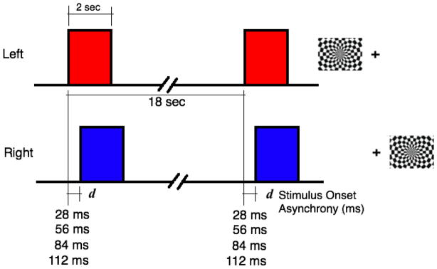
Event-related task paradigm for left (top row) and right (bottom row) hemifields and the corresponding checkerboard stimuli. The stimuli comprised two radial checkerboards separated by a fixation cross. To introduce delay in the onsets or the stimulus onset asynchrony (SOA), the left hemifield stimulus was presented d ms before the right. The SOA, d ranged from 0 to 112 ms (including 0, 28, 56, 84 and 112 ms) in steps of 28 ms, which was twice the time between screen refreshes of the projector.

Data Acquisition

After approval from the institutional review board (IRB) at Vanderbilt University, five healthy volunteers with normal vision were recruited to participate in the study. The subjects did not report any neurological or psychiatric conditions.

An initial whole-brain low-resolution PRESTO localizer (TR=2 s) was used to identify areas of visual cortex that responded to the block design stimuli comprising 20 s of left hemifield checkerboard flashing, 20 sec of right, and 20 sec of fixation cross (baseline) for five cycles. For the event-related experiments with stimulus onset differences, single-shot gradient-echo EPI (TR=250 ms, TE=25 ms, flip angle=30°, FOV=128 mm × 128 mm and voxel size=1mm × 1mm × 2mm) was used to acquire two coronal slices (with no slice gap) around the calcarine fissure region. The effective bandwidth in the phase encoding direction was 17 Hz and in the EPI frequency direction was 1458 Hz. Minimum time to acquire one slice was 125 ms due to constraints imposed by the combination of pulse sequence parameters. The images were acquired on a Philips Achieva 7T MR scanner using sensitivity encoding (SENSE factor=2) parallel imaging with a 16-channel receive coil and quadrature transmit coil and halfscan (HS=0.8). Stimulus presentation and fMRI volume acquisition were started at the same time. However, they were not synchronized trial-by-trial. Five functional runs with 0, 28, 56, 84 and 112 ms differences between the left and right hemifield onsets were acquired. The order of the runs presented to the subjects was randomized.

Data Preprocessing

We ran the data through a standard preprocessing pipeline, which included motion correction, linear trend removal and high-pass filtering. Although pure in-plane motion was unlikely to happen with coronal slices, it was necessary to ensure that any amount of motion did not blur small timing measurements. We observed less than 1 mm (spatial resolution) translational motion in the majority of runs. In some runs, the motion was above 1 mm. Motion correction was performed using the automated functional neuroimaging (AFNI- Robert Cox, Medical College of Wisconsin) software where the images in each run were registered in-plane to the first image in the run. The extracted signals from the concatenated runs were temporally filtered with a 120 s (0.0083 Hz) high-pass filter including detrending to remove low-frequency drifts and linear trends in the data. Low pass filtering may reduce the effects of cardiac and respiratory signals, but it may also remove important stimulus-related BOLD transitions relevant to Granger causality analysis. Hence no low pass filtering was performed. To preserve high spatial resolution, no spatial smoothing was performed.

Voxel Selection

Several methods for identifying task-related voxels in fMRI have been reported in the literature. These methods can be broadly classified into two categories: hypothesis-driven and data-driven methods. Statistical parametric mapping (SPM) is a commonly used hypothesis-driven method that uses a univariate multiple regression analysis and assumes a general linear model (GLM) for signals with a specific noise structure. It requires a priori knowledge about task paradigm, precise timing of stimulus onsets and an assumed hemodynamic response function (HRF) and performs linear convolution of the HRF with a deterministic stimulus timing function to construct reference functions. These modeling assumptions and the deterministic character assigned to the stimulus timing function may be too restrictive to capture a broad range of activation patterns and variability in stimulus-driven timings. SPM performs hypothesis testing on a voxel by voxel basis, which is massively univariate. Due to spatial coherence and temporal autocorrelation between brain voxels, meaningful activations occur in a cluster of voxels. So a multivariate approach may be more appropriate than the voxel by voxel approach for fMRI data analysis.

Data-driven methods follow a multivariate approach for exploratory fMRI analysis. Two of the most popular multivariate data-driven techniques applied for fMRI analysis are independent component analysis (ICA) and data clustering (e.g. K-means clustering, fuzzy clustering, hierarchical clustering, self-organizing map). They do not make any assumptions about HRF shape or require any prior knowledge about task paradigms. ICA works with higher-order statistics to separate maximally independent sources from fMRI data. It makes assumptions about strong independence between components in terms of mutual information (entropy) or non-Gaussianity that may result in biased decomposition (McKeown et al., 1998). K-means algorithm is limited by the assumption that the number of clusters is known a priori and that the clusters are spherically symmetric and separable in the feature space, which is not always applicable in the context of fMRI (Goutte et al., 1999). Self-organizing map (SOM) is an artificial neural network model that transforms data from high-dimension to low-dimension and reveals their natural cluster structures based on some similarity measure. It uses unsupervised learning to delineate clusters in data without any assumptions about their inherent relationships.

In our work, voxels were selected using self-organizing map (SOM) with a novel graph-based data visualization technique for cluster delineation (see Appendix B). This technique detects fine structures of clusters in the data and helps to identify relevant signals for the analysis (Katwal et al., 2011). We compared this approach with: a) independent component analysis (ICA), b) a general linear model (GLM) based multiple regression analysis using statistical parametric mapping (SPM8 - http://www.fil.ion.ucl.ac.uk/spm/software/spm8/), and c) a separate localizer scan using a block design stimulus paradigm. Voxels were selected from a single coronal slice to avoid slice-timing effects. For SOM, ICA and GLM methods, the functional runs were concatenated and voxels were selected from the concatenated time series. We manually selected a region around the calcarine fissure to exclude non-V1 voxels and assigned the selected voxels into right and left hemisphere categories. We made sure approximately equal numbers of voxels were picked from the left and the right hemispheres. For the localizer method, voxels responding to the on/off block stimulus from the block-design localizer scan were applied across all runs. Then we computed an average signal for each hemisphere. These average time course signals were used to assess their relative timings.

Voxel selection Using Self-organizing Map (SOM)

The preprocessed signals were used as inputs to the SOM algorithm to detect voxels responding to the task. The basic theory and description of the SOM algorithm are detailed in Appendix A. The total number of nodes, N, initial learning rate, α, and number of iterations for the SOM algorithm were chosen using the test for convergence procedure described by Peltier et al. (2003). A total number of 100 nodes (arranged in a 10×10, 2-D lattice grid), an initial learning rate of 0.2 and total 100 iterations were chosen for the analysis. We initialized the weight vectors associated with the nodes with first two principal components of the input data from the brain region. The winner node (best matching unit) was selected using the correlation coefficient metric:

$$\mathit{corr}(\mathit{x},{\mathit{m}}_c)=\underset{i}{max}\{\mathit{corr}(\mathit{x},{\mathit{m}}_i)\},i=1,\dots ,N$$ Eq. (2.1)

where corr(x, m_i) denotes the correlation coefficient between the input x (fMRI time series) and the weight vector of the i^th node, and corr(x, m_c) represents the correlation coefficient between the input x and m_c, weight vector of the best matching unit. The initial value of the full width at half maximum (FWHM) of the Gaussian kernel (σ) in the neighborhood function was set to be seven nodes, equal to the radius of the lattice (Peltier et al. 2003). Both learning rate (α) and neighborhood size (σ) were decreased exponentially with the increase in the learning iteration.

The training resulted in a 10×10 map of output nodes with a prototype and a voxel map for each node. Using our visualization scheme (see Appendix B), we delineated clusters on the map and picked the one whose voxel map included the calcarine fissure region.

Voxel selection Using Independent Component Analysis (ICA)

Independent component analysis (ICA) seeks to reveal spatiotemporal structures in fMRI data by discovering spatially (spatial ICA) or temporally (temporal ICA) independent components. Spatial ICA transforms each fMRI dataset into maximally independent components and identifies spatially non-overlapping and temporally coherent regions in brain (Calhoun et al., 2009). We used GIFT (Medical Image Analysis Lab, MIALAB), which implements spatial ICA, to extract task-related signals from the fMRI dataset. We concatenated sessions for each subject and ran the independent component analysis on the concatenated image using the FastICA algorithm incorporated in GIFT. At the end of the analysis, GIFT produced a number of components and their corresponding voxel map. The number of components was determined by the minimum description length (MDL) principle. To pick the task-related component, we examined the spatial map for each component and selected the one whose voxel map included the calcarine fissure region. Brain signals from the corresponding spatial map were extracted using a suitable threshold so that the total number of voxels from the region around the calcarine fissure matched the number obtained with SOM.

Voxel Selection Using Univariate General linear Model (GLM)

In this method, voxels were chosen from the concatenated time series for each subject using the GLM analysis of the event-related experiment. We constructed the regressor by convolving the event-related stimulus time series of the concatenated trials with a canonical hemodynamic response based on gamma variate functions. The model was fitted to the response using SPM8 and the regression parameter was estimated. A suitable threshold for the t-statistic was chosen so the total number of voxels from the activated region around the calcarine fissure was about the same as with other methods.

Voxel Selection with Localizer

A block stimuli comprising five cycles of right hemifield checkerboard (20 s), left hemifield checkerboard (20 s) and rest (fixation cross for 20 s) were presented to the subjects. The block stimulus time series was convolved with the hemodynamic response function using statistical parametric mapping (SPM8) to create an appropriate design matrix. The model was fitted to the response and regression parameter was estimated using SPM8. Activated regions in the left and right primary visual cortex were identified by contrasting left versus rest and right versus rest and using a FWE corrected p-value (<0.05). We used MarsBaR (Brett et al., 2002) to select a region of interest (ROI) each from the right and the left primary visual cortex regions including activated areas around the calcarine fissure. The MarsBaR selected only activated voxels from the selected region. We selected spherical region where the radius was chosen so the total number of activated voxels selected matched with other methods. The ROIs were applied across all functional runs to extract the signals for each session.

Detection of Timing Differences Using Granger Causality

A first order bi-variate autoregressive (AR) model was fitted to the average time series, x and y, from right and left hemispheres of V1, respectively. The Granger causality difference (GCD) F_x→y − F_y→x was then computed to assess the overall ability of x to predict y (Roebroeck et al., 2005 and Appendix C). In the absence of any overall temporal precedence, the GCD should be zero. A positive value of the GCD implies an ability of x to predict y or precedence of x over y and a negative value means the opposite. It should be emphasized the Granger causality measure was used to detect temporal shifts in BOLD responses and not to quantify any direct neuronal influences in this work.

Detecting Timing Differences Using Inverse Logit (IL) Model

To compare the results from Granger causality analysis, we used inverse logit (IL) functions to model the hemodynamic response. We fitted the model on the average BOLD responses from right and left hemispheres and estimated the timing parameters to compare the temporal differences.

To model the hemodynamic response function (HRF), a superposition of three inverse logit (sigmoid) functions, L(x)= (1+ e^−x)⁻¹, was used. The first function modeled the rise after activation, the second modeled the subsequent fall and undershoot, and the third function modeled the stabilization or return to baseline (Lindquist et al., 2009). The model of the HRF was given by:

$$h(t\mid \theta )={\alpha }_{1}L((t-T_1)/D_1)+{\alpha }_{2}L((t-T_2)/D_2)+{\alpha }_{3}L((t-T_3)/D_3)$$ Eq. (2.2)

Each function had three variable parameters representing the amplitude, position and slope of the response. The α_i parameter controlled the amplitude and direction of the curve, T_i controlled the position and D_i controlled the angle of the slope of the curve. We constrained the values of α₂ and α₃ (so that the fitted response begins at zero at the time point t=0 and ends at magnitude zero) and used a four parameter model where only the position of each function and the total amplitude were allowed to vary. We used following constraints for the amplitude:

$${\alpha }_3=\mid {\alpha }_2\mid -\mid {\alpha }_1\mid$$ Eq. (2.3)

and

$${\alpha }_2={\alpha }_1(L((-T_3)/D_3)-L((-T_1)/D_1))/(L((-T_3)/D_3)+L((-T_2/D_2))$$ Eq. (2.4)

We used a gradient descent solution to fit the model and used the parameter estimation procedure described by Lindquist et al. (2009) to calculate the height (H), time-to-peak (T), and full width at half maximum (W) from fitted HRF estimates. The difference in time-to-peak (TTPD) between right and left hemispheres was used to compare the temporal shift.

Statistical Inference

Conclusions about the significance of the GCD (F_x→y − F_y→x) and difference in time-to-peak (TTPD) measures were obtained by estimating the 95% confidence intervals using the time series block bootstrap (Efron and Tibshirani, 1993). This allows robust testing of the null hypothesis that GCD is equal to zero at the specific stimulus onset difference (SOA) for each subject. The time series were divided into individual trials and 1000 independent bootstrap samples were drawn randomly with replacement from the set of trials. The measures were then calculated on the reconstructed time series and 95% confidence intervals were determined. We used a bias-corrected accelerated (BCa) interval that adjusts the percentiles to correct for bias and skewness (Efron and Tibshirani, 1993).

We fitted a linear mixed-effects model to compare the GCD and TTPD measures with the stimulus onset differences (SOA). Granger causality in general is not a linear function of timing difference (Roebroeck et. al., 2005); however, in the time range of interest, the linear model is suitable for Granger causality difference. The GCD and TTPD yield measures of BOLD timing differences in different units. To allow direct comparison, the t statistic for the linear slope of the model was calculated to compare the precision of each method in terms of the standardized effect size. The precision compares the strength of the linear relationship against the amount of variability in the data. Similarly, the t statistic for the linear intercept was measured to compare the bias of the fits. The bias should be zero indicating that a zero BOLD timing difference produces a zero value of the measurement. Confidence intervals on the precision and bias estimates were generated using the case-resampling bootstrap.

Results

Identifying Task-related FMRI Signals

Analyses were conducted on the datasets for five subjects using four voxel selection methods to extract signals related to the fMRI task. Fig. 2 shows the 10×10 SOM output map with traces of node prototypes for a subject after applying the self-organizing map (SOM) algorithm. There are 100 nodes and their corresponding prototype time series arranged in a 2D map. In order to identify prototypes representing task-related signals, we used graph-based visualizations of the SOM output map. We used the combined connectivity (Fig. 3 (c)) obtained by merging the density-based connectivity (Fig. 3 (a)) and the correlation-based connectivity (Fig. 3 (b)) between node prototypes (described in appendix B) to reveal clusters in the data. The cluster containing task-related signals was identified from its voxel map. The cluster whose prototypes are shown in red traces in Fig. 3 (d) constituted voxels in the calcarine fissure region and chosen for our analysis. Voxels that were mapped to these prototypes are shown in Fig. 4 (a) after manual division into right hemisphere (red) and left hemisphere (blue) categories. The area denoted by ‘R’ is right V1. Voxels identified by other methods for the same subject after manual division into respective hemispheres are also shown in Fig. 4. The signals from voxels in these right and left hemisphere regions were averaged to create right and left hemisphere time series for further analysis. Fig. 5 shows average BOLD responses (averaged across trials) extracted by SOM from a subject when the stimulus onset difference was 112 ms.

Fig. 2.

The 10×10 matrix of prototypes from SOM output nodes. The arrows show labels of each block of the matrix. Each node is associated with a different set of voxels from the image slice, and the prototype traces correspond to the associated fMRI time series. The prototypes corresponding to task-evoked fMRI signals are towards the lower right-hand corner of the map. Note: The average of trials (18 seconds) of the prototype time series is shown here.

Fig. 3.

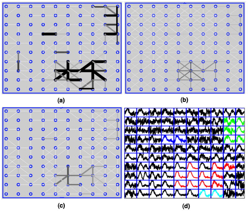
(a) Density-based connectivity visualization: Visualization of node connectivity based on local density distribution on the 10×10 SOM lattice. Connectivity is interpreted in gray scale where darker and wider lines mean strong connections. (b) Correlation-based connectivity visualization: Visualization of connectivity based on local correlation (correlation coefficient between the neighboring prototypes) on the SOM lattice. (c) Combined connectivity visualization: Visualization of connectivity based on local density distribution and local correlation on the SOM lattice. (d) The output map showing traces of prototypes in different colors for different clusters. The cluster shown in red traces whose voxel map included the calcarine fissure regions was chosen for our analysis.

Fig. 4.

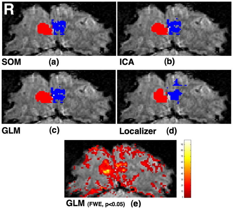
Voxels selected from V1 via (a) SOM (Voxel count: Right – 103, Left – 101), (b) ICA (Voxel count: Right – 102, Left – 103), (c) GLM (Voxel count: Right – 112, Left – 103), and (d) localizer scan (Voxel count: Right – 103, Left – 96). Voxels are shown after manual division into right hemisphere (red) and left hemisphere (blue) categories. (e) All activated voxels on the entire slice obtained using GLM analysis of the event-related experiment (SPM8).

Fig. 5.

Average trial BOLD responses from right and left hemispheres extracted by SOM for a subject at 112 ms SOA.

Granger Causality Can Detect Sub-100 ms Timing Differences From FMRI

We fitted a bivariate AR model of first order to the average time series from right and left V1 and calculated the Granger causality difference measures (GCD) F_x→y − F_y→x for different stimulus onset asynchronies (SOAs). Fig. 6 (a) shows the plot of the GCD measures versus SOA in five subjects for voxels selected by SOM. GCD was approximately zero at zero SOA and increased linearly with SOA as indicated by the linear mixed-effects model (dark line, p<0.00001). The color code represents results from 95% time series block bootstrap confidence intervals on each measure: blue indicates a “correct” conclusion and red “incorrect” for a test of the null hypothesis that GCD=0 for the specific subject at the specific SOA. For zero SOA, blue means the confidence interval included zero and for other SOAs, blue means its confidence interval excluded zero. Red indicates otherwise. Differences down to 28 ms were detectable in at least three subjects.

Fig. 6.

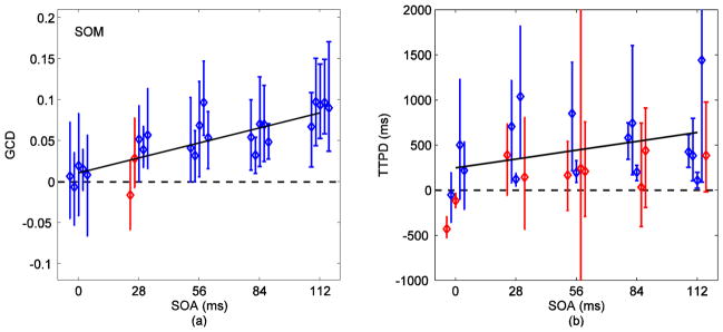
(a) Granger causality difference (F_x→y − F_y→x) versus stimulus onset asynchrony (SOA) for voxels selected via SOM. GCD was approximately zero at zero SOA and increased linearly with SOA as indicated by the linear mixed-effects model (dark line, p<0.00001). The color code represents results from 95% time series block bootstrap confidence intervals on each measure: blue indicates a “correct” conclusion and red “incorrect” for a test of the null hypothesis that GCD=0 for the specific subject at the specific SOA. For zero SOA, blue means the confidence interval included zero and for other SOAs, blue means its confidence interval excluded zero. Red indicates otherwise. Difference down to 28 ms was detectable in at least three subjects. (b) Time-to-peak differences (TTPD) from inverse logit (IL) fits on signals obtained via SOM. TTPD had a positive linear relationship with SOA (dark line) but it was statistically weak (p=0.27).

Fig. 7 (a) shows the GCD measures for voxels identified by ICA. GCD increased linearly with the increase in SOA (p=0.0006). However, there was a loss in sensitivity of GCD towards the stimulus onset differences when compared to results from SOM in Fig. 6 (a). Differences down to 84 ms were detectable in three out of five (60%) subjects while four subjects produced positive (greater than zero) GCD measures for differences down to 28 ms. Fig. 8 (a) shows the corresponding results with signals obtained from GLM. The 112 ms difference was detected in four (80%) subjects and differences down to 56 ms were detected in two (40%) subjects. The linear relationship of GCD with SOA for GLM was statistically weaker (dark line, p=0.008) than the relationship for SOM and ICA. For the localizer, 112 ms was detected in all subjects and differences down to 28 ms were resolved in two out of five (40%) subjects using GCD measures (Fig. 9 (a)). GCD was approximately zero for zero SOA and increased linearly with SOA (dark line, p=0.0001).

Fig. 7.

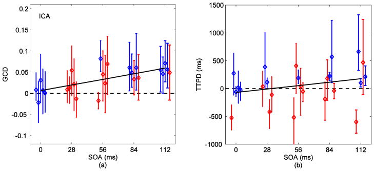
(a) GCD (F_x→y − F_y→x) versus SOA for voxels selected via ICA. The color code represents results from 95% time series block bootstrap confidence intervals on each measure (same as in Fig. 6). GCD was approximately zero at zero SOA and increased linearly with SOA as indicated by the linear mixed-effects model (dark line, p<0.0006). Loss of sensitivity of Granger causality in detecting timing differences in signals chosen from ICA (when compared to those from SOM in Fig. 6) was evident. Difference down to 84 ms was completely detected in three out of five (60%) subjects. Four subjects resulted in positive (greater than zero) GCDs for differences down to 28 ms. (b) TTPD from inverse logit (IL) fits on signals obtained via ICA. The linear relationship of TTPD with SOA (dark line) was stronger for ICA (p=0.08) than for SOM.

Fig. 8.

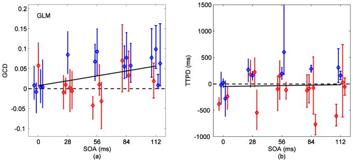
(a) GCD (F_x→y − F_y→x) versus SOA for voxels selected via GLM. The color code represents results from 95% time series block bootstrap confidence intervals on each measure (same as in Fig. 6). GCD at 0 ms stimulus onset asynchrony indicated positive bias in one subject. The 112 ms difference was detected in four (80%) subjects. Difference down to 56 ms was detected in two (40%) subjects. The linear relationship between GCD and SOA indicated by the linear mixed-effects model was weaker (dark line, p=0.008) than for SOM and ICA. (b) TTPD from inverse logit (IL) fits on signals obtained via GLM. The linear relationship between TTPD and SOA was statistically very weak (dark line, p=0.83).

Fig. 9.

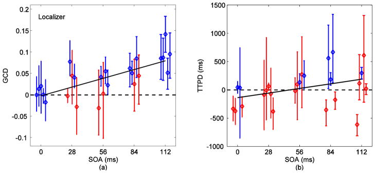
(a) GCD (F_x→y − F_y→x) versus SOA for voxels selected via localizer. The color code represents results from 95% time series block bootstrap confidence intervals on each measure (same as in Fig. 5). GCD was approximately zero at zero SOA and increased linearly with SOA as indicated by the linear mixed-effects model (dark line, p=0.0001). Differences down to 28 ms were detectable in two out of the five (40%) subjects. The 112 ms difference was detected in all subjects. (b) TTPD from inverse logit (IL) fits on signals obtained via localizer. The dark lines are linear mixed-effects model on the measures. TTPD increases linearly with SOA with p=0.02 (dark line).

In summary, GCD could resolve sub-100 ms differences. Differences as short as 28 ms, the shortest timing difference investigated, were resolved in individual subjects and most consistently with voxels selected by SOM.

Time-to-peak Difference (TTPD) Not As Consistent As Granger Causality Difference

Fig. 6 (b) shows the time-to-peak difference (TTPD) measures from inverse logit fits on the average signals obtained from SOM. The color code indicates results from 95% time series block bootstrap confidence intervals on each measure (same as in Fig. 6 (a)) for statistical inference. The estimated TTPDs did not follow the corresponding stimulus onset differences in absolute sense. However, the linear fit on the timing measurements indicated increase in measures with the increase in SOA. TTPD had a positive linear relationship with SOA but it was statistically weak (dark line, p=0.27). The linear relationship trend was evident with results for ICA (Fig. 7 (b), p=0.08) and localizer (Fig. 9 (b), p=0.02). With GLM (Fig. 8 (b)), the linear relationship between TTPD and SOA was obscure (p=0.83).

In summary, time-to-peak difference (TTPD) measures from inverse logit fits were not as stable and as consistent as the Granger causality difference measures in interpreting the temporal shifts in the signals.

Performance Comparison Using Precision and Bias Plots

To compare the performance of GCD and TTPD timing measurements from four voxel selection techniques, we fitted linear mixed-effects model on the timing measures and computed precision and bias of the fit for each method as described in the Methods section. Fig. 10 shows (a) precision and (b) bias of the fits for GCD and TTPD measures from all voxel selection techniques. The error bars indicate 95% confidence intervals from 2000 bootstrap samples. Two conclusions can be made from the precision plot: 1) Precision measures for GCD were higher than for TTPD for all voxel selection techniques. This meant that the sensitivity of the timing measurements for the stimulus-induced differences (SOA) and their linear relationship were stronger for GCD than for TTPD and 2) Voxels selected by SOM produced the highest precision value followed by localizer, ICA and GLM, in that order. The bias plot indicated that signals selected by SOM might be prone to higher bias than other techniques, especially with GCD timing measures. However, no strong conclusions can be made from their confidence intervals (Fig. 10 (b)). Localizer seemed to produce the least amount of bias with GCD measurements but a strong negative bias with TTPD measurements. We made an assessment of the impact of threshold or the number of voxels on the detectability of timing differences. The new results were in agreement with the presented results.

Fig. 10.

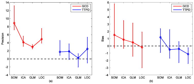
Performance comparison of the voxel selection methods using results from the linear mixed-effects modeling. (a) Precision was measured with the t statistic for the slope (linear term of the fit) describing the relationship to stimulus onset asynchrony. (b) Bias was measured with the t statistic for the intercept of the fit. The error bars indicate 95% confidence intervals from 2000 bootstrap samples generated using the case-resampling bootstrap.

In summary, GCD outperformed TTPD in the relative timing measurements and SOM outperformed ICA, GLM and localizer approach in selecting voxels contributing to the timing measurements in visual cortex.

Discussion

In this article, we assessed the ability to detect short BOLD timing differences from fMRI data. Brain images were acquired at ultrahigh field (7 T) and voxels responding to the task were identified with a multivariate data-driven approach using a novel visualization scheme for self-organizing map. We used a controlled slow even-related design that modulated the timing differences by controlling the visual stimuli onset delay. Based on our results, we reached the following conclusions: 1) Differences as small as 28 ms (the shortest investigated) were detectable in individual subjects in visual cortex using Granger causality as a measure of relative timings in conjunction with self-organizing map (SOM) as a voxel selection method, 2) Granger causality difference (GCD) outperformed time-to-peak difference (TTPD) from inverse logit fits for the detection of relative timings of BOLD responses in visual cortex, and 3) Self-organizing map (SOM) outperformed ICA, GLM and localizer approach in identifying task-related voxels for the detection of timing differences.

Benefits of Self-organizing map (SOM) on Detectability

The ability to detect small timing from fMRI data depends on the ability to identify task-related voxels in the data. FMRI data typically comprise a large noisy dataset where the magnitudes of detectable signals may be very low and signals of interest may be confined to a few voxels in the high-dimensional image space. The low contrast to noise ratios and spatial resolutions of fMRI challenge our ability in identifying task-related voxels critical for detecting small temporal differences. This demands a robust voxel selection strategy. A simple fixed anatomical region of interest (ROI) may not always ensure selection of important task-related signals constituting critical timing information, especially when the timing differences to be measured are small. The timing information in the task-induced signals may also have been muddled by late signals coming though draining veins.

For voxel selection in this study, we used two univariate methods: general linear model (GLM) and localizer scan that followed hypothesis-driven approach and two multivariate data-driven techniques: self-organizing map (SOM) and independent component analysis (ICA). The localizer and the GLM methods followed the conventional GLM-based multiple regression analysis using statistical parametric mapping (SPM) which performed linear convolution of the canonical double-gamma hemodynamic response function with the deterministic stimulus timing function to construct the reference function. These modeling assumptions and deterministic characteristics of the reference function may have been restrictive to capture the range of stimulus-driven BOLD transitions (Liao et al., 2008). This may have in effect diminished the power of Granger causality into detecting BOLD timing differences. Additionally, GLM and the localizer followed a voxel by voxel hypothesis testing approach that was massively univariate and unable to capitalize on neighborhood relationships or inter-voxel dependencies to improve sensitivity.

Our implementation of SOM used neighborhood correlation to group data based on similarities in their temporal patterns. The neighborhood function made use of inter-voxel relationships that increased its sensitivity. We used graph-based visualization scheme that delineates small structures of clusters in the data and helps in making correct timing assessments in fMRI by distinguishing early BOLD signals from late signals coming through draining veins etc. (Katwal et al., 2011). The other advantage of SOM, especially over GLM or similar model-based approach, is that it is unsupervised. It does not need the model of the response or stimulus timing information a priori but uses a machine learning approach for data analysis that is unsupervised and without any biases from assumptions. For ICA, we used spatial ICA that determined maximally independent components from the data by maximizing non-Gaussianity. This ensures segregation of task-related signals from other non-relevant signals and noise. Although data-driven, ICA made a strong assumption of independence between components which may have introduced bias and decreased its ability to detect task-related signals (Meyer-Bäse et al., 2004, McKeown et al., 1998). This may have resulted in the reduced power of ICA (compared to SOM) in capturing important BOLD transitions related to crucial timing information, which may in turn have produced lower sensitivity of ICA as suggested by the results (Fig. 7).

Importance of Granger Causality on Detectability

Granger causality has typically been formalized in terms of a multivariate autoregressive process that captures the temporal evolution of signals and reveals their interrelationships. This allows detection of small temporal shifts in signals from fMRI data, as shown by our results. However, regional variability in the HRF can affect the detectability of timing differences (Deshpande et al., 2010, Smith et al. 2011). Previous studies have suggested that the HRF shape and magnitude can vary across brain regions and individuals (Aguirre et al., 1998; Handwerker et al., 2004). On this premise, Deshpande et al. (2010) investigated the sensitivity of Granger causality analysis to HRF variability in single subjects concluding that fMRI could infer delays on the order of tens of milliseconds using Granger causality in the absence of HRF confounds (delay) across regions while an HRF delay can reduce the sensitivity of Granger causality to hundreds of milliseconds. In addition to this loss in sensitivity for true positives, the HRF variability may cause Granger causality analysis to result in spurious connection (false positive) between regions. In the assessment of temporal precedence in this work, the spurious connections may lead to the conclusion that signal A is preceding or following signal B when they have no temporal relationships in reality. While modulation of the activity (delays in this study) by experimental demands could cancel out the effect of hemodynamic variation and rule out such spurious findings (Roebroeck et al., 2005), results from simulation conducted by Schippers et al. (2011) using practical HRF models from Handwerker et al. (2004) suggested that such findings are actually rare and non-significant in a statistical sense.

The Granger causality difference (GCD) may reflect actual neuronal timing differences if a change in the experimental context (delays in our studies) modulates the measured differences ruling out hemodynamics as the cause of the results. The apparent linear relationship between SOA and BOLD timing measurements in this study is compelling evidence that the results are not an artifact of the hemodynamic variability and the measured BOLD timing differences can be attributed to the stimulus timing differences. This shows that Granger causality is capable of reflecting the relative timings of neuronal activities in visual cortex although it does not give absolute values of the timing differences in physical units. Results from the study conducted by Roebroeck et al. (2005) suggested that Granger causality is capable of revealing temporal precedence even if the time scale and delay is smaller than the sampling interval (TR). In this case, Granger causality may lose much of its sensitivity. But it still possesses enough power to detect interactions at a finer time scale (Roebroeck et al., 2005, Abler et al., 2006, Deshpande et al., 2010). This was indicated by successful measurements of delays smaller than the sampling time in our study as well. These findings validate the use of Granger causality in detecting short timing differences from fMRI data.

Detectability with Time-to-peak from Inverse logit Fit

The Granger causality difference compares signals and indicates their temporal precedence. A limitation of the method is that it does not measure timing differences in physical units. We wanted to see if the measured timing differences could follow the actual delay between the stimulus onsets. Our estimates of difference in time-to-peak (TTPD) parameters obtained from inverse logit fits did not reflect the corresponding stimulus onset differences, SOA (Figs. 6(b)–9(b)). Although there was some linear trend in the relationship between the two (as indicated by the linear fits), the measured values had some strong, random biases and variability. This is due to the fact that the hemodynamic response function is a complex, non-linear function of the neuronal or vascular changes and the HRF model (inverse logit functions) is limited in terms of its statistical accuracy for accurate recovery of the true response parameters (time-to-peak, width and height). This restricts accurate representation and may lead to unsystematic biases and confusion among the estimated response parameters (Lindquist et al., 2009). We examined the width and the height parameters (not shown here) for the right and left V1 BOLD responses. They matched closely for both hemispheres although not without some random bias and variability.

Previous studies suggest why time-to-peak measure from a hemodynamic model could be useful in the studies of timing in fMRI. Miezin et al. (2000) investigated hemodynamic response timing parameters and found that the time-to-peak estimate is stable across separate datasets for the same region within a subject and is a reliable measure of the hemodynamic response. A comparative study of the hemodynamic response models conducted by Lindquist et al. (2009) suggested that the inverse logit model is immune to a large degree of model misspecification and provides the least amount of bias and confusion between the response parameters than other models including canonical gamma and finite impulse response. Also, the use of a sparse event-related design helps to recover true response parameters. However, the presence of bias and confusion between estimated response parameters may challenge and deter accurate estimation, especially in the measurement of small timing differences.

The multivariate autoregressive model regresses the current value of a response onto its past values without having to estimate the shape of the hemodynamic response. This may have resulted in higher sensitivity of Granger causality measures than time-to-peak difference estimates in detecting small timing differences in this work.

Implications

The Granger causality analysis can be applied in conjunction with self-organizing map (SOM) for voxel selection to achieve higher sensitivity for detecting small temporal precedence in signals across brain regions. Our results showed that even sub-100-ms temporal differences could be resolved in visual cortex. Such capabilities may qualify fMRI for timing studies normally performed using EEG or MEG (Menon, 2012). This has important implications for decoding the temporal sequence of brain activations to better understand the neural dynamics of brain processes using fMRI. Our results may not generalize to studies involving different experimental conditions and regions of brain. A naïve computation of Granger causality to quantify temporal precedence across various regions in brain could be misleading. In particular, the variability in hemodynamic delay across brain regions could give misleading inferences on the actual delay. Our study focused on one region (calcarine fissure) of brain where voxelwise variability in hemodynamics may not have had much impact on measurement and interpretation of the actual delay. This may have increased sensitivity in measuring small delays in this study. However, the effect of hemodynamic variability may be more severe as we apply these methods in other cortical regions, e.g. between visual and motor cortex (Miezin et al., 2000). This will lead to loss in much of the sensitivity and accuracy in timing measurements. In this case, modulation of the delay by experimental demands and cognitive context become more relevant to rule out hemodynamics as the cause of the results and validate the measured timing differences. In summary, with careful consideration of experimental design, these methods may be adapted to studies related to detecting relative timings of brain activity using fMRI.

Conclusions

In this work, we assessed the ability to detect small differences in the timings of brain activities from fMRI data. High-resolution fMRI data were acquired from primary visual cortex (V1) with a 7 T MR scanner. A data-driven approach using graph-based visualizations of self-organizing map (SOM) was used to identity voxels responding to the task. Voxels were also selected using independent component analysis (ICA), a general linear model (GLM) based multiple regression analysis and localizer scans in conjunction with GLM. Granger causality analysis was performed to detect temporal differences on the average signals. Additionally, we fit curves to the average signals using inverse logit functions and measured time-to-peak differences to compare temporal differences in the signals. The combination of SOM and Granger causality outperformed others by detecting timing differences as small as 28 ms between left and right hemispheres in individual subjects. This combination also generated highest precision at a moderate bias. In summary, sub-100 ms (as small as 28 ms) timing differences were detected in BOLD responses in visual cortex. SOM outperformed ICA, GLM and localizer methods in identifying task-related voxels and Granger causality offered highest sensitivity for detecting small timing differences from fMRI data.

Highlights.

• We detect small differences in the timings brain activities using fMRI.

• We follow data-driven approach for voxel selection using self-organizing map.

• SOM outperforms ICA, GLM and localizer approaches for signal extraction.

• Granger causality can detect timing differences as small as 28 ms in visual cortex.

Appendix A. Self-organizing Map

The self-organizing map (SOM) is an artificial neural network model that maps high-dimensional input data into a set of nodes arranged in a low-dimensional (often a 2-D) rigid lattice using unsupervised learning (Kohonen, 1990; Kohonen, 2001). A weight vector of the same dimension as the input data vector is associated with each node of SOM. The SOM algorithm constitutes a series of training steps that tune the weight vectors of the nodes to the input data vectors. At each step, the input vector is compared with each of the nodes to find the best matching unit (BMU). The BMU refers to the node whose weight vector is the closest match of the input vector. Once the best matching unit is determined, the weights of the BMU and its surrounding nodes are adjusted. The magnitude of this adjustment decreases with time (iteration) and for nodes away from the BMU. This results in an effective visualization and abstraction of high-dimensional data for exploratory data analysis.

The SOM Algorithm

The self-organizing map (SOM) algorithm constitutes two major steps: 1) determining the best matching unit (BMU) and 2) updating the weight vectors associated with the BMU and some of its neighbors. Prior to training, the weight vectors associated with each node of the map are suitably initialized. For a profitable initialization, the vectors can be sampled evenly from the subspace spanned by the two largest principal components eigenvectors (Kohonen, 2001). The training expands over several iterations and is based on competitive learning. In each iteration, a vector x =[x₁, x₂, …, x_n]^T (where n is the length of fMRI data in this work) is chosen from the input space. The weight vectors of the nodes m_i = [m_i1, m_i2, …, m_in]^T (where i=1, …, N ; N being the total number of nodes) are compared with x to determine the best matching unit (BMU) based upon a similarity metric. The most commonly used metric is the Euclidean distance:

$$\left|\right|\mathit{x}-{\mathit{m}}_c\left|\right|=\underset{i}{min}\left\{\right||\mathit{x}-{\mathit{m}}_i|\left|\right\},i=1,\dots ,N$$ Eq. (A.1)

where || || represents the Euclidean norm, x is the vector under consideration, m_i denotes the weight of the i^th node on the map and m_c represents the weight of the BMU. Once the BMU is determined, the weight vectors associated with the BMU and some of its neighbors in the map are updated using:

$${\mathit{m}}_i(t+1)={\mathit{m}}_i(t)+h_{ci}(t)[\mathit{x}(t)-{\mathit{m}}_i(t)]$$ Eq. (A.2)

where t is the current iteration number; h_ci(t) is defined as the neighborhood kernel which controls the number of neighboring nodes to be updated and the rate of update in each iteration. As the iteration progresses, the neighborhood function shrinks the neighborhood size. In general, the neighborhood kernel takes the form of a Gaussian function:

$$h_{ci}(t)=\alpha (t)exp\left(-{\left|\right|r_i-r_c\left|\right|}^2/2{\sigma }^2(t)\right)$$ Eq. (A.3)

where r_i and r_c are spatial co-ordinates of the i^th node and the winner node (BMU), respectively, in the output space; σ is the full width at half maximum (FWHM) of the Gaussian kernel that determines the neighboring nodes to be updated. α denotes the learning rate which controls how fast the weights get updated. Both σ and α decrease monotonically with the increase in the learning iteration, t. The iteration continues until convergence is reached when further iterations produce no node changes. At the end of training, it generates a learned SOM. Each node in the SOM has an associated weight vector, also called prototype, and its input vectors map. As applied to our fMRI data, the input vectors were the voxel time series and the output nodes each had an associated time series (prototype) and its voxel map.

Appendix B. Graph-based Visualizations of SOM

The SOM maps high-dimensional data into a low-dimensional lattice grid through an adaptive vector quantization that results in orderly arrangement of the prototypes in the output space based on their similarities. However, a postprocessing scheme is required to capture cluster boundaries in the data via SOM. In this work, we identified voxels of interest from fMRI data using a combination of two graph-based visualization techniques that incorporated i) local density distribution across SOM prototypes (density-based connectivity) and ii) local similarities (correlations) between the prototypes (correlation-based connectivity) (Katwal et al., 2011). The combined connectivity visualization effectively captures cluster boundaries and delineates task-related signals and their connectivity structures.

Visualization of Density-based Connectivity

The density-based connectivity visualization is realized by draping the connectivity matrix, CONNDD, over the SOM lattice (Taşdemir, 2010). The existence of an edge between two prototypes m_i and m_j on the graph indicates that they are neighbors in the input data space and the weight of the connection between them gives its connectivity strength:

$$\text{CONNDD}(i,j)=\left|{RF}_{ij}\right|+\left|{RF}_{ji}\right|i,j=1,2,\dots ,N$$ Eq. (B.1)

|RF_ij| denotes the number of input vectors in the receptive field of prototype m_i for which m _j is the second BMU (m_i being the first BMU). The connectivity strengths can be normalized to one by dividing each value with the mean of the strongest connection of each prototype (Taşdemir, 2010). Any stronger connections will be assigned a value of one. Fig. 3 (a) shows the visualization of density-based connectivity on the output map (Fig. 2). The strength of the connection was indicated in gray scale and binned width where wider and darker connections represented strong connectivity strengths. Any connectivity strengths smaller than the mean connectivity strength of the sixth strongest connections were omitted to discard noise and outliers (Taşdemir, 2010). The mean connectivity strength dropped sharply after the sixth rank.

Visualization of Correlation-based Connectivity

The correlation coefficient matrix, CONNCC, which includes temporal similarities (correlation coefficients) of neighboring prototypes, can be visualized graphically to display correlation-based connectivity. We used the normalized correlation coefficient values between prototypes as measures of their local similarities (Fig. 3 (b)). The strength of the connection between prototypes was visualized in gray scale where dark lines represented strong correlations.

Combined Connectivity Visualization

For combined connectivity visualization, the two connectivity matrices: CONNDD and CONNCC are multiplied (element-by-element).

$$\text{CONNDDCC}(i,j)=\text{CONNDD}(i,j)\times \text{CONNCC}(i,j)$$ Eq. (B.2)

The resulting visualization, obtained by draping CONNDDCC, suppresses the visualization of noise and delineates detailed connectivity structures of task-related signals (Katwal et al., 2011). The combined connectivity visualization on our data delineated clusters shown in Fig. 3 (c).

Appendix C. Granger Causality

Granger causality gives the measure of directed influence one signal or a region exerts over another. Originally introduced by Granger for causality analysis in econometric models (Granger, 1969) and later mathematically formalized in terms of vector autoregressive (VAR) models by Geweke (1982), Granger causality is based on the idea of temporal precedence. If the past values of signal in region A help in predicting the future values of signal in region B, then A is said to Granger-cause B. Granger causality was introduced for brain connectivity studies by Goebel et al. (2003) and since has been used in many fMRI related brain connectivity studies. A more detailed review of Granger causality in fMRI could be found in Deshpande et al. (2010) and Schippers et al. (2011). Granger causality analyzes temporal precedence to reveal the direction of influence across brain areas. By showing whether the signal change in one area precedes or follows the signal change in another area, Granger causality may indicate temporal differences between signals.

A vector time series x[n] (where n represents time) can be modeled by a vector autoregressive (VAR) process (Goebel et al., 2003) as:

$$\mathit{x}[n]=\sum _{k=1}^p{\mathbf{A}}_x[k]\mathit{x}[n-k]+\mathit{u}[n]$$ Eq. (C.1)

where A_x[k] are the autoregressive (AR) coefficients which regress x[n] onto its own past; p is the model order and u[n] is white noise whose cross-covariance matrix is given by:

$$var(\mathit{u}[\text{n}])={\mathbf{\sum }}_1$$ Eq. (C.2)

In the same manner, a second vector time-series y[n] can be modeled as:

$$\mathit{y}[n]=\sum _{k=1}^p{\mathbf{A}}_y[k]\mathit{y}[n-k]+\mathit{v}[n]$$ Eq. (C.3)

where

$$var(\mathit{v}[n])={\mathbf{T}}_1$$ Eq. (C.4)

The bivariate model for $\mathit{z}[n]=\left[\begin{array}{c}\mathit{x}[n]\\ \mathit{y}[n]\end{array}\right]$ is given by:

$$\mathit{z}[n]=\sum _{k=1}^p{\mathbf{A}}_z[k]\mathit{z}[n-k]+\mathit{w}[n]$$ Eq. (C.5)

where

$$var(\mathit{w}[n])=\mathbf{Y}=\left[\begin{array}{cc}{\mathbf{\sum }}_2& C\\ C^{\text{T}}& {\mathbf{T}}_2\end{array}\right]$$ Eq. (C.6)

The residual covariance matrices Σ₁, T₁ and T₂ are useful in quantifying the ability to predict the current values of x and y based upon their past values. In terms of VAR model, the measure of degree to which the time-series x predicts (Granger causes) y is given by:

$$F_{x\to y}=ln\left(\right|{\mathbf{T}}_1|/|{\mathbf{T}}_2\left|\right)$$ Eq. (C.7)

where T₁ and T₂ are residual variances of y in the univariate model and the bivariate model, respectively.

Similarly, the ability of y to predict x is given by:

$$F_{y\to x}=ln\left(\right|{\mathbf{\sum }}_1|/|{\mathbf{\sum }}_2\left|\right)$$ Eq. (C.8)

Σ₁ and Σ₂ being residual variances of x in the univariate and the bivariate models, respectively. F_x→y and F_y→x take the values in the interval [0, Inf) and are non-negative.

References

- Abler B, Roebroeck A, Goebel R, Höse A, Schönfeldt-Lecuona C, Hole G, Walter H. Investigating directed influences between activated brain areas in a motor response task using fMRI. Magnetic Resonance Imaging. 2006;24:181–185. doi: 10.1016/j.mri.2005.10.022. [DOI] [PubMed] [Google Scholar]
- Aguirre GK, Zarahn E, D’esposito M. The variability of human, BOLD hemodynamic responses. NeuroImage. 1998;8:360–369. doi: 10.1006/nimg.1998.0369. [DOI] [PubMed] [Google Scholar]
- Brett M, Anton JL, Valabregue R, Poline J-B. Region of interest analysis using an SPM toolbox. Proceedings of the 8th International Conference on Functional Mapping of the Human Brain; Sendai, Japan. 2002. [Google Scholar]
- Calhoun VD, Liu J, Adali T. A review of group ICA for fMRI data and ICA for joint inference of imaging, genetic, and ERP data. NeuroImage. 2009;45:S163–S172. doi: 10.1016/j.neuroimage.2008.10.057. [DOI] [PMC free article] [PubMed] [Google Scholar]
- Deshpande G, Sathian K, Hu X. Effect of hemodynamic variability on Granger causality analysis of fMRI. NeuroImage. 2010;52:884–896. doi: 10.1016/j.neuroimage.2009.11.060. [DOI] [PMC free article] [PubMed] [Google Scholar]
- Efron B, Tishbirani RJ. An introduction to the bootstrap. Chapman and Hall; New York: 1993. [Google Scholar]
- Formisano E, Goebel R. Tracking cognitive processes with functional MRI mental chronometry. Current Opinion in Neurobiology. 2003;13:174–181. doi: 10.1016/s0959-4388(03)00044-8. [DOI] [PubMed] [Google Scholar]
- Geweke J. Measures of conditional linear dependence and feedback between time series. Journal of the American Statistical Association. 1982;77:304–313. [Google Scholar]
- Goebel R, Roebroeck A, Kim D, Fomisano E. Investigating directed cortical interactions in time-resolved fMRI data using vector autoregressive modeling and Granger causality mapping. Magnetic Resonance Imaging. 2003;21:1251–1261. doi: 10.1016/j.mri.2003.08.026. [DOI] [PubMed] [Google Scholar]
- Goutte C, Toft P, Rostrup E, Nielsen FA, Hansen LK. On clustering fMRI time series. Neuroimage. 1999;9:298–310. doi: 10.1006/nimg.1998.0391. [DOI] [PubMed] [Google Scholar]
- Granger CWJ. Investigating causal relations by econometric models and cross-spectral methods. Econometrica. 1969;37:424–438. [Google Scholar]
- Handwerker DA, Ollinger JM, D’Esposito M. Variation of BOLD hemodynamic responses across subjects and brain regions and their effects on statistical analyses. NeuroImage. 2004;21:1639–1651. doi: 10.1016/j.neuroimage.2003.11.029. [DOI] [PubMed] [Google Scholar]
- Henson RNA, Price CJ, Rugg MD, Turner R, Friston KJ. Detecting latency differences in event-related BOLD responses: application to words versus nonwords and initial versus repeated face presentations. NeuroImage. 2002;15:83–97. doi: 10.1006/nimg.2001.0940. [DOI] [PubMed] [Google Scholar]
- Hernandez L, Badre D, Noll D, Jonides J. Temporal sensitivity of event-related fMRI. NeuroImage. 2002;17:1018–1026. [PubMed] [Google Scholar]
- Katwal SB, Gatenby JC, Gore JC, Rogers BP. Minimum resolvable latency difference of BOLD responses at 7T using autoregressive modeling. Proceedings of the 17th Annual Meeting, International Society for Magnetic Resonance in Medicine; Hawaii, USA. 2009. p. 3677. [Google Scholar]
- Katwal SB, Gore JC, Rogers BP. Analyzing fMRI data with graph-based visualizations of self-organizing maps. 2011 IEEE International Symposium on Biomedical Imaging: From Nano to Macro; Chicago, USA. 2011. pp. 1577–1580. [Google Scholar]
- Kohonen T. The Self-organizing map. Proceedings of the IEEE. 1990;78:1464–1480. [Google Scholar]
- Kohonen T. Series in Information Sciences 30. New York: Springer-Heidelberg; 2001. Self-organizing maps. [Google Scholar]
- Liao W, Chen H, Yang Q, Lei X. Analysis of fMRI data using improved self-organizing mapping and spatio-temporal metric hierarchical clustering. IEEE Transactions on Medical Imaging. 2008;27:1472–83. doi: 10.1109/TMI.2008.923987. [DOI] [PubMed] [Google Scholar]
- Liao CH, Worsley KJ, Poline JB, Aston JAD, Duncan GH, Evans AC. Estimating the delay of the fMRI response. NeuroImage. 2002;16:593–606. doi: 10.1006/nimg.2002.1096. [DOI] [PubMed] [Google Scholar]
- Lindquist MA, Loh JM, Atlas LY, Wager TD. Modeling the hemodynamic response function in fMRI: Efficiency, bias and mis-modeling. NeuroImage. 2009;45:S187–S198. doi: 10.1016/j.neuroimage.2008.10.065. [DOI] [PMC free article] [PubMed] [Google Scholar]
- Lin F-H, Polimeni JR, Tsai KW-K, Witzel T, Chang W-T, Kuo W-J, Belliveau JW. The limit of relative timing accuracy of BOLD fMRI in human visual cortex. Proceedings of the 19th Annual Meeting, International Society for Magnetic Resonance in Medicine; Montréal, Québec, Canada. 2011. p. 3582. [Google Scholar]
- McKeown MJ, Makeig S, Brown GG, Jung TP, Kindermann SS, Bell AJ, Sejnowski TJ. Analysis of fMRI data by blind separation into independent spatial components. Human Brain Mapping. 1998;6:160–188. doi: 10.1002/(SICI)1097-0193(1998)6:3<160::AID-HBM5>3.0.CO;2-1. [DOI] [PMC free article] [PubMed] [Google Scholar]
- Menon RS. Mental chronometry. NeuroImage. 2012;62:1068–1071. doi: 10.1016/j.neuroimage.2012.01.011. [DOI] [PubMed] [Google Scholar]
- Menon RS, Kim SG. Spatial and temporal limits in cognitive neuroimaging with fMRI. Trends in Cognitive Sciences. 1999;3:207–216. doi: 10.1016/s1364-6613(99)01329-7. [DOI] [PubMed] [Google Scholar]
- Menon RS, Luknowsky DK, Gati JS. Mental chronometry using latency-resolved functional MR. Proceedings of the National Academy of Sciences of the United States of America. 1998;95:10902–07. doi: 10.1073/pnas.95.18.10902. [DOI] [PMC free article] [PubMed] [Google Scholar]
- Meyer-Bäse A, Wismüller A, Lange O. Comparison of two exploratory data analysis method for fMRI: Unsupervised clustering versus independent component analysis. IEEE Transactions on Information Technology in Biomedicine. 2004;8:387–398. doi: 10.1109/titb.2004.834406. [DOI] [PubMed] [Google Scholar]
- Miezin FM, Maccotta L, Ollinger JM, Petersen SE, Buckner RL. Characterizing the hemodynamic response: effects of presentation rate, sampling procedure, and the possibility of ordering brain activity based on relative timing. NeuroImage. 2000;11:735–759. doi: 10.1006/nimg.2000.0568. [DOI] [PubMed] [Google Scholar]
- Peltier SJ, Polk TA, Noll DC. Detecting low-frequency functional connectivity in fMRI using a self-organizing map (SOM) algorithm. Human Brain Mapping. 2003;20:220–226. doi: 10.1002/hbm.10144. [DOI] [PMC free article] [PubMed] [Google Scholar]
- Raj V. PhD Dissertation. Yale University; United States: 2001. Studies of physical limitations in functional magnetic resonance imaging. (Publication No. AAT 3007413) [Google Scholar]
- Roebroeck A, Formisano E, Goebel R. Mapping directed influence over the brain using Granger causality and fMRI. NeuroImage. 2005;25:230–242. doi: 10.1016/j.neuroimage.2004.11.017. [DOI] [PubMed] [Google Scholar]
- Rogers BP, Katwal SB, Morgan VL, Asplund CL, Gore JC. Functional MRI and multivariate autoregressive models. Magnetic Resonance Imaging. 2010;28:1058–1065. doi: 10.1016/j.mri.2010.03.002. [DOI] [PMC free article] [PubMed] [Google Scholar]
- Schippers MB, Remco R, Keysers C. The effect of intra- and inter-subject variability of hemodynamic response on group level Granger causality analyses. NeuroImage. 2011;57:22–36. doi: 10.1016/j.neuroimage.2011.02.008. [DOI] [PubMed] [Google Scholar]
- Sigman M, Jobert A, Lebihan D, Dehaene S. Parsing a sequence of brain activations at psychological times using fMRI. NeuroImage. 2007;35:665–668. doi: 10.1016/j.neuroimage.2006.05.064. [DOI] [PubMed] [Google Scholar]
- Smith SM, Miller KL, Salimi-Khorshidi G, Webster M, Beckmann CF, Nichols TE, Ramsey JD, Woolrich MW. Network modelling methods for FMRI. NeuroImage. 2011;54:875–891. doi: 10.1016/j.neuroimage.2010.08.063. [DOI] [PubMed] [Google Scholar]
- Taşdemir K. Graph based representations of density distribution and distances for self-organizing maps. IEEE Transactions on Neural Networks. 2010;21:520–526. doi: 10.1109/TNN.2010.2040200. [DOI] [PubMed] [Google Scholar]