Rare variant detection using family-based sequencing analysis

Abstract

Next-generation sequencing is revolutionizing genomic analysis, but this analysis can be compromised by high rates of missing true variants. To develop a robust statistical method capable of identifying variants that would otherwise not be called, we conducted sequence data simulations and both whole-genome and targeted sequencing data analysis of 28 families. Our method (Family-Based Sequencing Program, FamSeq) integrates Mendelian transmission information and raw sequencing reads. Sequence analysis using FamSeq reduced the number of false negative variants by 14–33% as assessed by HapMap sample genotype confirmation. In a large family affected with Wilms tumor, 84% of variants uniquely identified by FamSeq were confirmed by Sanger sequencing. In children with early-onset neurodevelopmental disorders from 26 families, de novo variant calls in disease candidate genes were corrected by FamSeq as Mendelian variants, and the number of uniquely identified variants in affected individuals increased proportionally as additional family members were included in the analysis. To gain insight into maximizing variant detection, we studied factors impacting actual improvements of family-based calling, including pedigree structure, allele frequency (common vs. rare variants), prior settings of minor allele frequency, sequence signal-to-noise ratio, and coverage depth (∼20× to >200×). These data will help guide the design, analysis, and interpretation of family-based sequencing studies to improve the ability to identify new disease-associated genes.

Challenges in using whole-genome sequencing (WGS) data for identifying rare DNA variants responsible for heritable disease include high false negative (FN) rates and the need to minimize the number of false positive (FP) variants to reduce the total number of variants for subsequent validation. Family-based sequencing designs have been applied to gene discovery for several diseases (1–3). Methods for calling variant positions in DNA sequence data include short oligonucleotide analysis package 2 (SOAP2) (4), sequence alignment/map tools (Samtools) (5), and genome analysis toolkit (GATK) (6, 7). When assessing data from related individuals, simple filtering can remove variants that do not conform to Mendelian transmission expectations, thereby reducing FPs. However, this approach does not reduce the frequency of FNs, and it removes all de novo mutations (8). There are approaches that borrow information across neighboring variants through family-based haplotype phasing (9, 10). As an orthogonal approach, integrating Mendelian inheritance and raw data of family members at a single position can reduce both FPs and FNs and has been implemented in variant calling tools for family trios (9, 11). In recent simulation studies, Li et al. (12) showed that joint variant calling in data from extended families will further improve detection of Mendelian variants and reduce FP de novo mutations. However, a limitation of their study is that simulations cannot incorporate many sources of variations that are observed across millions of positions within a sample and across samples and families. Their study did not evaluate variant positions with base coverage greater than 40×, nor compare data generated by targeted versus WGS; they did not compare the performance of family-based calling for founder versus nonfounder or for common versus rare variants. Thus, evaluation of a family-integrated method under real settings across many individuals is required to prevent underestimation of its actual contributions to identifying rare variants in families.

In addition, accurate variant calling and decreased FN rates (FNRs) enable the development of more efficacious and efficient studies that incorporate decisions about study design (who should be sequenced first in a large family and at what sequencing coverage), data analysis (setting up unknown parameters), and results interpretation (distinguishing true variants from FPs for functional association). Knowledge of factors contributing to accurate variant calling in families facilitates these decisions.

We have developed a family-based variant calling program (Family-Based Sequencing Program, FamSeq) that provides a confidence measure for variant calls using data from all family members and builds on Bayesian networks (13) and the Markov chain Monte Carlo (MCMC) algorithm (14). We used this method to perform simulation studies and analyze sequencing data from 28 families [one from the HapMap (Haplotype Map) project, one with Wilms tumor (WT), and 26 with mitochondrial neurodevelopmental disorders] presenting various pedigree structures. Compared with variant calling using a single-individual-based method or using only a family trio (14%), FamSeq reduced FN variant calls by 33% in the extended HapMap pedigree. In the analysis of actual data from one family, FamSeq resulted in the identification of an additional ∼300 to ∼1,200 new variant positions in WGS that otherwise would have been undetected using the Single method.

Our goal is to provide a method for rare variant detection and to guide the design and analysis of a family-based sequencing study. We describe and validate our method, then describe simulations and analyses of 92 samples from 28 families. We present a comprehensive investigation of factors that may determine the improvements achievable by our family-integrated method on a per-person and per-position basis. We also illustrate the effect of annotating Mendelian variants in studying either dominant or recessive traits.

Results

FamSeq.

Fig. 1 describes the FamSeq framework. This method provides a confidence measure for genotype calls, which is a posterior probability Pr(G_i|D,P). Here G denotes genotype, i denotes an individual, P denotes pedigree structure, and D is a vector that denotes sequencing data, including read counts, base quality, and mapping quality, for all n family members (individual i and relatives). Incorporating data from family members, Pr(G_i|D,P) allows for accurate variant calling when the data from person i are not informative, perhaps due to a weak signal-to-noise-ratio, by borrowing strength from all relatives (Fig. 1B). Here we measure the signal-to-noise-ratio using the ratios of the likelihood estimates (Pr(D_i|G_i)) for the two most likely genotypes. FamSeq has included probabilities of de novo mutations. It allows for variable pedigree size (n > 3) and structure. In addition to using the Elston-Stewart algorithm as in Li et al. (12) for pedigree analysis, we implemented two unique approaches, Bayesian network and MCMC. The Bayesian network approach directly calculates joint probabilities for each combination of genotypes of all family members and allows for analytic calculation in pedigrees with marriage loops and/or consanguinity, as long as they form directed acyclic graphs. This method gives faster computation than the Elston-Stewart algorithm with or without loops in pedigrees of size less than 7. The MCMC method allows for the use of continuous probability density functions as priors on the genotype probability and likelihood , instead of designating the point mass a priori.

Fig. 1.

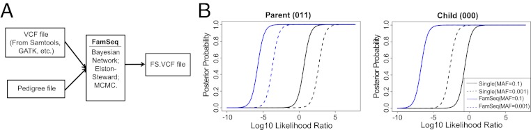
Illustration of variant calling using FamSeq. (A) FamSeq variant calling framework. (B) Two examples in a family trio. We use 0 to denote reference and 1 to denote heterozygous variant. The order of genotypes presented in the parentheses is father, mother, and child. In both cases, FamSeq gives the child a high posterior probability (>0.9) for the true genotype even when the child has a relatively low log10 LLR. This is done in FamSeq by borrowing strength from data of the parents.

Motivating Example: Family with Inherited WT.

Familial transmission of predisposition to WT, a childhood kidney tumor, is consistent with an autosomal dominant mutation with incomplete penetrance. Two predisposition genes have been localized by genetic linkage studies, but neither gene has been identified (15). We generated WGS data for five members of a large WT family and focused on a 5.6 MB linkage region on chr19q. Because genetic linkage has been previously demonstrated, the two distantly related individuals WTX524-708 and WTX524-000 are expected to share the same Mendelian variants as individuals WTX524-709 and WTX524-004 in the trio (Fig. 2). Comparing FamSeq with GATK (with variant recalibration), we found that both methods identified 4,920 positions with variant calls in all four affected family members. FamSeq identified an additional 132 positions and GATK uniquely identified one position.

Fig. 2.

A family with Wilms tumor for genomic sequencing of 19q13-linked region. The family trio is affected mother (WTX524-004), unaffected father (WTX524-029), and affected child (WTX524-709). Two affected distant relatives (WTX524-708, WTX524-000) are also sequenced.

Sanger Validation.

To assess the validity of the FamSeq uniquely called variants, we performed Sanger sequencing on 57 of the 132 positions, which exist in a subregion and meet an additional requirement of presenting reference calls in the unaffected father. This four-variants-plus-one-reference filtering procedure is designed to prioritize variants potentially important for WT and was performed on both FamSeq and GATK-based calls. We obtained reliable Sanger results on 38 FamSeq-unique positions and confirmed that 32 (61 variant calls) are true (SI Appendix, Table S1). Our validation rate is 61/73 = 84% (95% confidence interval: 75–92%). Among the confirmed FamSeq-unique variants, 17 (53%) are rare (not reported or at a minor allele frequency of less than 5%). Other than one position where FamSeq corrected a call from the variant by GATK to reference in the unaffected father, the FamSeq-unique positions were missed by GATK because they were (i) called as reference in one affected individual, (ii) removed during variant quality score recalibration, or (iii) had variant calls at a tranche level of 99.9–100 or lower.

Using simulated and actual data, we identified variables that determine the possible improvements from using our family-based analysis. From here on, we compare FamSeq with the Single method based on their posterior probabilities. First, we describe the results based on simulations.

Genotype Configurations.

FamSeq improved the accuracy in all Mendelian genotypes (15 scenarios for a family trio, Fig. 3A) and made substantial improvements in two scenarios: (i) at positions where all family members have reference genotypes, FamSeq corrected FP calls (∼30%; SI Appendix, Fig. S1), and (ii) at positions where a single parent and child carry heterozygous variants, FamSeq corrected FN calls (20–40%; SI Appendix, Fig. S1). FamSeq identified true Mendelian positions that were erroneously called as variants by the Single method, as shown by the red cells in the heatmap of Fig. 3A. For example, at truth = 000, FamSeq reduced discordant calls of 001; at truth = 101, again FamSeq reduced discordant calls of 001 and 102, made by the Single method. When the de novo mutation rate is high [1 × 10⁻⁵, compared with variants with minor allele frequency (MAF) of 0.01; SI Appendix, Fig. S1B], FamSeq missed 34% of true de novo mutations correctly called by the Single method, suggesting possible underestimations. We made similar observations with a family quartet.

Fig. 3.

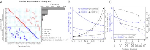
Simulation results. (A) Highlighted results from a full simulation of all possible genotype configurations of a family. Each row is the simulated genotype for the family trio (father, mother, child). Here, 0 is homozygous reference, 1 is heterozygous variant, and 2 is homozygous variant. Each heatmap entry is the percent reduction in discordance from using the Single method to using FamSeq. The values on the diagonal are equal to the sum of all other 63 values in the same row. Only 27 columns are shown. Additionally, there are 37 columns with genotypes containing “no calls.” The corresponding complete results can be found in SI Appendix, Fig. S1. The barplot on the right presents the frequency for observing each configuration. (B) Targeted simulation to evaluate effect of MAF. F stands for FamSeq and S stands for single method. (C) Targeted simulation to evaluate effect of pedigree size and structure.

MAF.

The MAF parameter is used for computing prior probabilities of genotypes, Pr(G), in FamSeq and the Single method and is mostly unknown (Fig. 3B). Setting different values of MAF (from 10⁻⁵ to 0.5) switches the balance between the FNR and FPR in the Single method. As MAF increases, FNRs decrease and FPRs increase. With FamSeq, not only are both error rates lower at all values, but as the MAF varies, the changes in FNRs and in FPRs in the children, and changes in FNRs in the parents, are much attenuated; that is, error rates are less dependent on MAF values. Therefore, by jointly calling variants in all family members, we can set the same MAF at all base positions, for example 0.001, without compromising the detection of true variants.

Family Size and Pedigree Structure.

Starting from a parent–child pair, FamSeq reduced both FNR and FPR when we included the second parent (family size = 2 to size = 3), and then added another sibling (size = 3, 4) (Fig. 3C). Interestingly, adding more children (size = 4, 5, 6) did not further reduce error rates, whereas adding the grandparents (size = 5–7) made additional reductions in both FNR and FPR. When the parental data are not available, we also observed improvements made by FamSeq in analyzing all siblings together (size = 3, FNR 23.5% vs. 13.3%, FPR 0.5% vs. 0.4%). This has important implications when prioritizing individuals from a larger pedigree to accurately and comprehensively detect rare DNA variants.

Contribution to Family Members.

The reduction in error rates using FamSeq is membership-dependent (Fig. 3 B and C). FNRs are better controlled in parents than in children. FPRs are better controlled in children than in parents (founders), which reduces the cost of subsequent sequence verifications. Both reduce the FPs in calling de novo mutations in children. Accordingly, when grandparents’ data are available, the FPRs in the corresponding parent (nonfounder) decrease substantially, which improves the detection of de novo mutations in children.

Next, we present results from the analysis of sequencing data in extended families (SI Appendix, Table S2).

WGS Data Analysis.

We analyzed a three-generation HapMap WGS dataset of five samples. In the whole genomes of HapMap samples, FamSeq found 1,179, 317, and 494 new variant positions across all samples when analyzing pedigrees g3 (grandparent trio), c3 (child trio), and a5 (all five). Within each sample, FamSeq called ∼7,000 to ∼32,000 more variants than the Single method. Samples with lower coverage (NA12892 at ∼25×; SI Appendix, Tables S2 and S3) benefited most from FamSeq analysis, exhibiting a greater percentage of increased variant calls.

HapMap Sample Validation.

In three samples (mean coverage ∼25–30×), we compared FamSeq calls with HapMap calls at ∼1 million single-nucleotide polymorphism (SNP) positions (16) (SI Appendix, Table S3). Homozygous genotypes are more easily identified than heterozygous variants (17). Using known SNP data, we combined all homozygous SNP positions as true negatives and used all heterozygous SNP positions as true positives, from NA12878, NA12891, and NA12892 (∼400,000 true positives for each sample). As expected, FamSeq called more positions at high confidence (7–29% fewer no call positions) and identified more true variants with percent reduction in FNs of 14–33%, and without substantially increasing the number of false discoveries (1–3%; Fig. 4A and SI Appendix, Table S3). In particular, comparing pedigrees c3 and a5, we observed a statistically significant difference in the percent reduction of FNs (15% vs. 33% in NA12878, P < 0.0001). This result is consistent with simulations comparing sizes of 5 and 7 in the parent (Fig. 3C). We also observed low sensitivity to varying MAF values in variant calling when using FamSeq (SI Appendix, Fig. S2). In contrast to the simulations, we did not observe a decrease in FPs in the child (NA12878 in g3). One explanation is we derived the input likelihood estimates from GATK, which may aggressively filter out FPs, but at a price of missing some true positives.

Fig. 4.

Analysis of sequencing data in extended pedigrees. (A) HapMap SNP validation (SI Appendix, Table S3). (B) FamSeq-unique variants found in 45 people (parents) in 25 families affected with mitochondrial disorders. (C) Coverage versus LLR in TS samples. All positions called concordantly by the Single method and FamSeq are shown in the background as a smoothed scatterplot. Red circles represent FamSeq-unique variants; black triangles represent Single-unique variants.

This validation was performed at HapMap SNP positions, including all common SNPs whose known genotypes may have been used for calibration by GATK. Additionally, most of these SNPs (98%) are located in the noncoding region. Therefore, we look for larger improvements from using FamSeq for finding rare DNA variants at sequence sites where variant calling in the Single method has not been optimized.

Targeted Sequencing Data Analysis in Families with Mitochondrial Neurodevelopmental Disorders.

These families vary in size from 2 to 7 and include single-parent, nuclear, as well as three-generation families (SI Appendix, Table S2). In each individual, we sequenced 524 nuclear-encoded mitochondrial candidate genes (18, 19) and focused our analysis on 962 Kb of coding regions in autosomes. We observed a significant increase in new variants called by FamSeq in the parents (Fig. 4B and SI Appendix, Table S4; FamSeq vs. Single method at size = 3: Kolmogorov-Smirnov test P < 0.001; FamSeq vs. Single method at size = 4: P < 0.001; FamSeq at size = 3 vs. size = 4: P < 0.001, FamSeq at size = 4 vs. size > 4, P = 0.06). We measured the significantly increased number of variants as related to family size in a total of 45 individuals from 25 different families, thus accounting for biological and technological variations between different sequenced individuals. We are currently validating these positions using Sanger-based sequencing, which may facilitate finding the unknown gene defects in these families. We did not observe significant increases in variants in the children (Fig. 3C and SI Appendix, Fig. S3). However, the approximate reduction in FNRs (estimated by % FamSeq-unique variants) in the three-generation pedigree was 1–5%, which is substantially larger than the 0.1% observed at HapMap SNP positions (SI Appendix, Table S5) indicating the power of FamSeq in detecting rare variants. In three of these families, we found 15 unique variant positions (SI Appendix, Table S5) that are not reported in the Single Nucleotide Polymorphism Database (dbSNP) or the 1,000 Genomes Project, nine of which are nonsynonymous. We also analyzed family MTF04 in three ways: trio, trio plus either pair of grandparents, and trio plus both pairs of grandparents. Interestingly, compared with the Single method for this family, only the extended pedigree (size = 5 or 7) analysis found new positions in the affected child. This illustrates the limitation of the Single method in detecting rare DNA variants and demonstrates the power of using multigeneration pedigrees to detect rare variants.

Coverage and Log Likelihood Ratios.

FamSeq improved variant calling in both WGS and targeted sequencing (TS) data at mean base coverages from 25× to 1,200×. In the HapMap WGS data (mean coverage 25–60×), FamSeq improved accuracy primarily at positions with low-to-moderate coverage (15–20×; Table 1 and SI Appendix, Fig. S4). NA12892 had the lowest mean coverage (25×) and presented the biggest reduction in error rates among the three samples (Fig. 4A). Compared with the WGS data, the TS data have a wider range of mean coverage (200–1,200×). However, FamSeq still called 1.2% more variants overall, at coverage from 11 to 600× (median 24×; Fig. 4C and SI Appendix, Fig. S3). To explore why, we correlated base coverage with log likelihood ratio (LLR) (input for FamSeq) in all sequence data. We expected a genotype-specific linear relationship between LLR and coverage (SI Appendix, Fig. S5, r = 0.87 for heterozygotes, r = 0.80 for homozygous positions), which can be derived analytically from the underlying binomial distribution used by Samtools and GATK (20). FamSeq strengthens signals at positions with a low LLR (LLR < 10). Therefore, it can improve variant calling in sequencing data at positions with coverage 20× or lower. However, in TS data where most positions are at high coverage, FamSeq called more variants in 381 positions, 234 (61%) of which have high coverage (>20×) but still low LLR (<10), and thus show a relationship that varies from the expected linear relationship (Fig. 4C and SI Appendix, Fig. S5).

Table 1.

Mean base coverage of all loci with HapMap heterozygous calls in FamSeq performance categories

	FamSeq
Single	Concordant	Discordant	N
Concordant	32 (sd = 10, n = 1.3M)	51 (sd = NA, n = 1)	16 (sd = 7, n = 126)
Discordant	16 (sd = 7, n = 254)	25 (sd = 11, n = 1784)	14 (sd = 8, n = 74)
N	15 (sd = 7, n = 658)	16 (sd = 8, n = 55)	14 (sd = 7, n = 758)

Cells in bold are where FamSeq improved on Single method (sd, standard deviation; n, the number of loci in each category).

Discussion

We have developed a family-integrated method, FamSeq, which uses Mendelian transmission information to inform the calling of variants in raw sequence data. Such joint variant calling has been reported to improve variant detection using simulated data (12). In simulations, we identified factors that may affect the level of improvements made by FamSeq, including family genotype configurations, the prior setting of MAF, as well as pedigree size and structure. Using actual sequence data from 28 families, we also evaluated the performance of FamSeq in practical settings, using WGS (WT family) or TS (families with mitochondrial disorders) to determine the effect of variables such as known SNPs versus unknown variants and moderate (20×) versus high sequencing coverage (>200×). By looking across 45 samples from 25 families, we accounted for biological and technical variations in real data and observed a statistically significant increase in variant detection with an increase in family size. From our comparative analysis of data with truth from two different studies using WGS, we found that FamSeq increased the sensitivity of variant calling, while still maintaining specificity. We project that the application of FamSeq to sequencing data for rare variant detection in families with heritable diseases will yield significant improvements at low, moderate, and high sequencing coverage.

To be of practical use, variant calling algorithms that use family data should be computationally efficient and also account for marriage loops and/or consanguinity. FamSeq uses a Bayesian network to compute posterior probabilities, which results in fast computation (in minutes for analyzing WGS data) with a family size less than 7. The use of parallel probability calculations will extend the utility of the Bayesian network approach to larger families.

To allow for uncertainty in the estimates of LLRs, which will further improve variant calling accuracy, FamSeq includes an MCMC approach. The LLRs represent the signal-to-noise information from each family member. In 3,600 SNP positions where both the Single method and FamSeq made mistakes, the coverage as well as LLRs are higher than the average values, suggesting a possible bias in the LLR estimates (SI Appendix, Fig. S4). Thus, when variances on the LLR estimates are available, our MCMC approach may be useful to correct variant calling at more positions. Similarly, variances on the MAF estimates can be incorporated when available.

The overall improvement by FamSeq is measured on a continuous scale as increased confidence in the correct call for a variant or reference position. FamSeq gives a posterior probability as the confidence measure for variant calls. We compared this with two confidence measures derived from GATK. First, we examined the quality tranches that used HapMap SNP truths to define cutoffs; second, the individual-based posterior probability at positions that passed our hard-filtering criteria. We used the quality tranches in analyzing the WGS data for the WT family and used a cutoff at the last tranche level: 99.9–100 (less specific than other levels). We used posterior probabilities in the other analyses and a cutoff at 90%, because these analyses are either for comparison with HapMap SNPs or for TS data (where quality tranches cannot be reliably generated). We considered any call with a confidence measure at or below the cutoff as a “no call.” In the HapMap data, FamSeq reduced the overall no call rate at the SNP positions by giving reference or variant calls at higher confidence (SI Appendix, Table S3). Changing cutoffs can shift the balance between the FNR, FPR, and no call rate in the Single method and in the comparison with FamSeq. Regardless of the cutoffs, FamSeq provides a confidence measure that incorporates family information and, compared with the Single method, better describes the uncertainty of individual genotype calls, which improves the overall accuracy.

We identify two key questions for balancing cost with obtaining adequate data to identify the disease variant of interest. (i) Who should be selected from a large family for initial sequencing? (ii) At what coverage depth should selected family members be sequenced? FN variant calls are of great concern in these types of gene identification studies. We found that adding both parents and then grandparents before adding more siblings was most effective. One explanation is when the LLRs for the parents are similar but only one parent has a heterozygous variant, adding data from one set of grandparents (the parents of one parent) can break the tie and help identify which parent carries the variant, whereas adding data from more children cannot. Additionally, we determined that WGS data generated at an average of 25–30× coverage per person will most benefit from FamSeq analysis. While overall coverage in the WT data were ∼30×, about 5–20% of all base positions had a coverage of <20× nevertheless. FamSeq was highly beneficial in correcting calling errors made at these positions (Table 1). In sequencing data (especially TS data) generated at an overall high coverage (200–1,200×), FamSeq is still valuable for variant calling as there will still be positions with low coverage and also positions with high coverage but small LLR (<10). These outlier positions are likely caused by sequence-specific technical errors, allelic imbalance, or other unobservable factors.

We identified factors that can facilitate the analysis and interpretation of family sequencing studies. Using simulations with FamSeq analysis, we showed the choice of MAF had little effect on the FNRs and FPRs in children, and the FNRs in parents, but can still affect the FPRs in parents (Fig. 3C). This remaining effect can be alleviated in two ways: (i) setting an MAF of 0.001 or less to control for the FPR, while maintaining the power to detect true variants by using FamSeq, and (ii) prefiltering FP positions, which appear to be implemented in GATK for HapMap SNPs (SI Appendix, Fig. S2; little reduction in FPR by FamSeq was observed with the HapMap sample originally processed by GATK). For comparison, we observed FamSeq substantially reduced the FPR in HapMap SNPs on data generated by Samtools, which is less suited to removing FPs.

In both simulations and real data (Fig. 3A and SI Appendix, Figs. S1 and S4 and Table S3), we showed that FamSeq can mistakenly change calls from the individual-based method, although this happens rarely compared with the corrections it makes (1–3% vs. 14–33% in HapMap SNPs, P < 0.001). Therefore, when comparing results from the Single method and FamSeq, we suggest giving high priority to positions at which FamSeq changed a de novo mutation to either a Mendelian mutation or to a reference position, or added variant calls in parents or removed them in children. This prioritization needs to be integrated into the generation of lists of validation variants. In general, family-based analysis improves both sensitivity and specificity of calling Mendelian mutations. However, in the case of de novo mutation calls, this decrease in FPs may increase FNs in some occasions.

We studied two diseases, one with a dominant trait and one with suspected recessive inheritance. For the family affected with WT (autosomal dominant), we took advantage of the large pedigree (Fig. 2) and previous linkage mapping and used a 3+2 design: a family trio with affected parent and child and two affected distant relatives. Sequence variants identified in the affected mother and son and two other relatives but not in the unaffected parent are candidates for follow-up analysis. For further sequencing, we prioritized the grandparents of the trio to uncover additional variants. Linkage information was not available for the families with mitochondrial disease, which is a genetically and clinically heterogeneous (18) group of disorders, making disease-related gene discovery very challenging. One approach relies on filtering against public SNP databases for genes with two rare functional variants (homozygous or compound heterozygous) present only in the affected individuals (1). Notably, an analysis of our targeted sequence data of 524 genes identified relatively more recessive candidate genes in the larger families (e.g., MTF04) compared with smaller families. These positions are being validated.

Our method is implemented in a C++ based software called FamSeq, which is freely available. It can process variable pedigree structures and accommodate de novo mutations. It contains three approaches: a Bayesian network, an MCMC algorithm, and the Elston-Stewart algorithm. For a variant call format (VCF) file containing 3.5 M variant positions for a pedigree of seven members without loops [on an Intel(R) Xeon(R) processor with a CPU at 2.93 GHz], the respective computing times are 550 s, 550 s, and 10,000 s (10,000 iterations) for the Bayesian network, Elston-Stewart, and MCMC, respectively. When a loop is added to this pedigree, we observe little change in computing times for the Bayesian network and MCMC methods, but can increase time of at least 20–50% for loop-cutting within the Elston-Stewart algorithm (21). FamSeq is a stand-alone module that can be integrated with existing analysis pipelines of data generated from different high-throughput platforms, both sequencing-based and array-based data (5–7, 17). Our method can be extended to give joint posterior probabilities for calling short indels in sequenced families (6). Thus, FamSeq provides a fascile and flexible means of reducing FN sequence calls, and will greatly aid in identifying disease-causing variants in next-generation sequencing studies.

Methods

Individual-Based (Single) Method.

Let D_i denote the raw sequencing measurements—that is, read counts, read quality, and mapping quality—and G_i denote the genotype for sample i. For a family of n members, we use to denote a vector { and a vector {. GATK⁵ provides likelihood estimates in VCF files. By following Bayes’ rule, the genotype posterior probabilities are calculated as , where the prior is the expected genotype frequency in the population, and is calculated based on the MAF and Hardy-Weinberg equilibrium.

Family-Based Method (FamSeq).

Let denote the pedigree structure. We calculate a genotype posterior probability , which incorporates the actual pedigree structure and raw sequencing data and accommodates de novo mutations. We use three methods to compute : a Bayesian network, and Elston-Stewart and MCMC algorithms. FamSeq provides an updated VCF file that includes the family-based variant calling results and posterior probabilities.

Bayesian Network.

By treating the entire pedigree as a Bayesian network, we write the posterior probabilities as , where and denote the genotype of sample i’s father and mother. If sample i is the founder of the family, . If sample i is not the founder, we calculate through Mendelian transmission. We allow for de novo mutations by assigning to each parental allele a probability of m for acquiring a new alteration in the germline. For example, when both parents’ genotypes are homozygous reference, the probability of their child having a heterozygous variant would be , rather than 0. We set the default mutation rate m as 1e-7 (11).

MCMC Method.

We used the Gibbs sampler (22) to derive posterior probabilities. The full conditionals are shown below:

where is all possible genotypes for all relatives of sample i in the pedigree denotes the genotype of sample i’s jth child, denotes the genotype of the other parent of sample i’s jth child, and J_i denotes the total number of children of sample i. This method allows us to sample and from probability distributions, rather than set them at fixed values.

Full Simulation.

To evaluate the contribution of family-based analysis to improving variant calling accuracy, we simulated all genotype configurations for a family trio and a family quartet. First, we simulated the two parents’ genotypes at known MAFs. Then based on the parents’ genotypes, we simulated the children’s genotypes according to Mendelian transmission and allowing for de novo mutations. We then simulated likelihoods from the density functions of bivariate normal distributions for each genotype [where μ is equal to (1.7,1.7), (0,0), and (−1.7, −1.7) for the three genotypes, and Σ is equal to (0.3,0.15; 0.15,0.3) for homozygous and (0.45,0.225; 0.225,0.45) for heterozygous genotypes]. We performed this simulation using two settings: (i) MAF = 0.2, m = 1e-3, 10 million iterations, and (ii) MAF = 0.01, m = 1e−5, 100 million iterations. We then calculated likelihoods at the true and at (0.1,0.05; 0.05,0.1). We used different variance matrices to account for additional technical effects that cannot be observed and estimated.

Targeted Simulation.

To evaluate the impact of pedigree size, structure, and MAF, we fixed the genotype configurations to extensions of (father = 0, mother = 0, child = 0) and (father = 0, mother = 1, child = 1), and simulated the raw intensity data based on bivariate normal distributions for each genotype. For pedigree size and structure, we considered the following scenarios: size = 2, parent–child pair; size = 3, family trio; size = 4, nuclear family with two children; size = 5, nuclear family with three children; size = 6, nuclear family with four children, or nuclear family with three children and one grandparent; and size = 7, two grandparents, two parents, and three children. For MAF, we considered 0.5, 0.2, 0.1, 0.05, 0.01, 1e−3, 1e−4, and 1e−5. For each scenario, we repeated the simulation for 1 million times. There are two different groups, one for computing the FPRs and one for computing the FNRs. We computed the FPRs in individuals carrying homozygous references and computed the FNRs in individuals carrying heterozygous variants. When there is only one parent/grandparent, the parent/grandparent is 1. When there are two parents/grandparents, one parent/grandparent is 1 and the other is 0.

WGS Data.

We downloaded the WGS data of NA12891, NA12892, and NA12878 from the 1000 Genomes Project (www.1000genomes.org), and NA12877 and NA12882 sequence data from the Sequence Read Archive (www.ncbi.nlm.nih.gov/Traces/sra). The data for the first three samples are generated using GAII and those for the other two are generated using HiSeq2000. We downloaded the consistent calls from the HapMap Phase II and III merged genotype data for NA12891, NA12892, and NA12878 (http://hapmap.ncbi.nlm.nih.gov). Using HiSeq2000, we also conducted WGS of five samples (one trio plus two distant relatives) from a large pedigree that presented with Wilms tumor. Our analysis focused on a 5.6 MB linkage region in Chr19q. In WGS analysis, we filtered out bases that are noted as simple repeats or segmental duplications by the University of California, Santa Cruz human genome assembly hg19, and those with total allelic counts less than 10.

TS Data.

We performed DNA sequence capture of 524 nuclear-encoded mitochondrial genes (19) from 92 samples in 26 families (SI Appendix, Table S2) and multiplex-sequenced all capture libraries using Illumina HiSeq2000, except for MTF04-b, c, and d, which were sequenced using MiSeq. Our analysis focused on a 762 KB region of autosomes.

Methods Evaluation.

We calculated the FNR as the rate of reference or no calls for a true variant genotype, and the FPR as the rate of variant calls for a reference genotype. We defined concordance as having genotype calls that are identical to the HapMap truth, and discordance as having genotype calls that are different from the HapMap truth.

Unique Variant Calls of FamSeq and the Single Method.

We combined the posterior probability of the heterozygous variant with that of the homozygous variant to evaluate the number of unique variant calls added by either FamSeq or the Single method. We designated a call as a unique variant call if the method of interest changes the calls from those of the alternative method in the following ways: reference to variant, no call to variant, or reference to no call. See SI Appendix for further information on sequencing data analysis pipeline and Sanger experiments.

References

- 1.Ng SB, et al. Exome sequencing identifies the cause of a mendelian disorder. Nat Genet. 2010;42(1):30–35. doi: 10.1038/ng.499. [DOI] [PMC free article] [PubMed] [Google Scholar]
- 2.Glazov EA, et al. Whole-exome re-sequencing in a family quartet identifies POP1 mutations as the cause of a novel skeletal dysplasia. PLoS Genet. 2011;7(3):e1002027. doi: 10.1371/journal.pgen.1002027. [DOI] [PMC free article] [PubMed] [Google Scholar]
- 3. Koenekoop RK, et al. (2012) Mutations in NMNAT1 cause Leber congenital amaurosis and identify a new disease pathway for retinal degeneration. Nat Genet 44(9):1035–1039. [DOI] [PMC free article] [PubMed]
- 4.Li R, et al. SOAP2: An improved ultrafast tool for short read alignment. Bioinformatics. 2009;25(15):1966–1967. doi: 10.1093/bioinformatics/btp336. [DOI] [PubMed] [Google Scholar]
- 5.Li H, et al. 1000 Genome Project Data Processing Subgroup The Sequence Alignment/Map format and SAMtools. Bioinformatics. 2009;25(16):2078–2079. doi: 10.1093/bioinformatics/btp352. [DOI] [PMC free article] [PubMed] [Google Scholar]
- 6.DePristo MA, et al. A framework for variation discovery and genotyping using next-generation DNA sequencing data. Nat Genet. 2011;43(5):491–498. doi: 10.1038/ng.806. [DOI] [PMC free article] [PubMed] [Google Scholar]
- 7.McKenna A, et al. The Genome Analysis Toolkit: A MapReduce framework for analyzing next-generation DNA sequencing data. Genome Res. 2010;20(9):1297–1303. doi: 10.1101/gr.107524.110. [DOI] [PMC free article] [PubMed] [Google Scholar]
- 8.Roach JC, et al. Analysis of genetic inheritance in a family quartet by whole-genome sequencing. Science. 2010;328(5978):636–639. doi: 10.1126/science.1186802. [DOI] [PMC free article] [PubMed] [Google Scholar]
- 9.Zhou B, Whittemore AS. Improving sequence-based genotype calls with linkage disequilibrium and pedigree information. The Annals of Applied Statistics. 2012;6(2):457–475. [Google Scholar]
- 10.Roach JC, et al. Chromosomal haplotypes by genetic phasing of human families. Am J Hum Genet. 2011;89(3):382–397. doi: 10.1016/j.ajhg.2011.07.023. [DOI] [PMC free article] [PubMed] [Google Scholar]
- 11.Conrad DF, et al. 1000 Genomes Project Variation in genome-wide mutation rates within and between human families. Nat Genet. 2011;43(7):712–714. doi: 10.1038/ng.862. [DOI] [PMC free article] [PubMed] [Google Scholar]
- 12.Li B, et al. A likelihood-based framework for variant calling and de novo mutation detection in families. PLoS Genet. 2012;8(10):e1002944. doi: 10.1371/journal.pgen.1002944. [DOI] [PMC free article] [PubMed] [Google Scholar]
- 13.Pearl J. Causality. New York: Cambridge Univ Press; 2000. [Google Scholar]
- 14.Lin S, Thompson E, Wijsman E. An algorithm for Monte Carlo estimation of genotype probabilities on complex pedigrees. Ann Hum Genet. 1994;58(Pt 4):343–357. doi: 10.1111/j.1469-1809.1994.tb00731.x. [DOI] [PubMed] [Google Scholar]
- 15.McDonald JM, et al. Linkage of familial Wilms’ tumor predisposition to chromosome 19 and a two-locus model for the etiology of familial tumors. Cancer Res. 1998;58(7):1387–1390. [PubMed] [Google Scholar]
- 16.Altshuler DM, et al. International HapMap 3 Consortium Integrating common and rare genetic variation in diverse human populations. Nature. 2010;467(7311):52–58. doi: 10.1038/nature09298. [DOI] [PMC free article] [PubMed] [Google Scholar]
- 17.Wang W, et al. Identification of rare DNA variants in mitochondrial disorders with improved array-based sequencing. Nucleic Acids Res. 2011;39(1):44–58. doi: 10.1093/nar/gkq750. [DOI] [PMC free article] [PubMed] [Google Scholar]
- 18.Scharfe C, et al. Mapping gene associations in human mitochondria using clinical disease phenotypes. PLOS Comput Biol. 2009;5(4):e1000374. doi: 10.1371/journal.pcbi.1000374. [DOI] [PMC free article] [PubMed] [Google Scholar]
- 19.Shen P, et al. High-quality DNA sequence capture of 524 disease candidate genes. Proc Natl Acad Sci USA. 2011;108(16):6549–6554. doi: 10.1073/pnas.1018981108. [DOI] [PMC free article] [PubMed] [Google Scholar]
- 20.Li H, Ruan J, Durbin R. Mapping short DNA sequencing reads and calling variants using mapping quality scores. Genome Res. 2008;18(11):1851–1858. doi: 10.1101/gr.078212.108. [DOI] [PMC free article] [PubMed] [Google Scholar]
- 21.Stricker C, Fernando RL, Elston RC. Linkage analysis with an alternative formulation for the mixed model of inheritance: The finite polygenic mixed model. Genetics. 1995;141(4):1651–1656. doi: 10.1093/genetics/141.4.1651. [DOI] [PMC free article] [PubMed] [Google Scholar]
- 22.Geman S, Geman D. Stochastic relaxation, gibbs distributions, and the bayesian restoration of images. IEEE Trans Pattern Anal Mach Intell. 1984;6(6):721–741. doi: 10.1109/tpami.1984.4767596. [DOI] [PubMed] [Google Scholar]
Associated Data
This section collects any data citations, data availability statements, or supplementary materials included in this article.