

Abstract
Evolution of prokaryotes involves extensive loss and gain of genes, which lead to substantial differences in the gene repertoires even among closely related organisms. Through a wide range of phylogenetic depths, gene frequency distributions in prokaryotic pangenomes bear a characteristic, asymmetrical U-shape, with a core of (nearly) universal genes, a “shell” of moderately common genes, and a “cloud” of rare genes. We employ mathematical modeling to investigate evolutionary processes that might underlie this universal pattern. Gene frequency distributions for almost 400 groups of 10 bacterial or archaeal species each over a broad range of evolutionary distances were fit to steady-state, infinite allele models based on the distribution of gene replacement rates and the phylogenetic tree relating the species in each group. The fits of the theoretical frequency distributions to the empirical ones yield model parameters and estimates of the goodness of fit. Using the Akaike Information Criterion, we show that the neutral model of genome evolution, with the same replacement rate for all genes, can be confidently rejected. Of the three tested models with purifying selection, the one in which the distribution of replacement rates is derived from a stochastic population model with additive per-gene fitness yields the best fits to the data. The selection strength estimated from the fits declines with evolutionary divergence while staying well outside the neutral regime. These findings indicate that, unlike some other universal distributions of genomic variables, for example, the distribution of paralogous gene family membership, the gene frequency distribution is substantially affected by selection.
Keywords: gene frequency distribution, steady genome model, goodness of fit, evolution mechanisms
Introduction
Comparative genomics of prokaryotes (archaea and bacteria) provides compelling evidence that the genomes of these organisms are in incessant flux (Snel et al. 2002; Dagan et al. 2008; Koonin and Wolf 2008). Through common and intensive processes of gene loss and gene gain via horizontal gene transfer, gene repertoires of prokaryotes typically diverge rapidly, much faster than the sequences of highly conserved genes that are traditionally used for phylogeny construction, such as ribosomal RNA or ribosomal proteins (Snel et al. 2002; Kunin and Ouzounis 2003; Mirkin et al. 2003; Dagan et al. 2008). As a result, even prokaryotes with (nearly) identical sequences of conserved genes that are classified as strains of the same species often substantially differ in their gene repertoires (Akopyants et al. 1998; Lawrence and Hendrickson 2005; Medini et al. 2005; Kettler et al. 2007; Rasko et al. 2008; Tettelin et al. 2008; Ishmael et al. 2009; Reno et al. 2009; Touchon et al. 2009; den Bakker et al. 2010; Mira et al. 2010). The first to be discovered and by now textbook case of such major interstrain differences involves laboratory and pathogenic strains of Escherichia coli that may differ by as many as 30% of their genes due to the acquisition of so-called pathogenicity islands by the pathogenic strains (Perna et al. 2001; Kudva et al. 2002; Zhang et al. 2007).
At the other end of the spectrum, when genomes of distant prokaryotes, for example, archaea and bacteria, are compared, the fraction of readily identifiable orthologous genes is a small minority of the respective gene sets (Koonin and Wolf 2008). The core set of universally conserved genes is tiny, less than 100, and slowly but steadily shrinking with the growth of the number of sequenced genomes (Koonin 2003; Charlebois and Doolittle 2004; Puigbò et al. 2009).
Collectively, these findings on the fluidity of the prokaryotic gene repertoires led to the concept of pangenome, which may be defined as the totality of the genes found in a particular clade and is sometimes viewed as a new paradigm in microbial genomics (Tetz 2005; Rasko et al. 2008; Mira et al. 2010; Karberg et al. 2011).
Pangenomes can be defined at any phylogenetic depth, from all prokaryotes to strains of a single species or even isolates of a single strain. The diversity of gene repertoires can be quantitatively summarized in a gene frequency distribution, that is, the probability ck that a randomly picked gene is found in precisely k out of K genomes (Baumdicker et al. 2010; Collins and Higgs 2012). Remarkably, the gene frequency distribution shows a characteristic asymmetric U-shape regardless of the phylogenetic depth at which a pangenome is analyzed (Koonin 2011b). All gene frequency distributions consist of a core of common genes (cK), numerous unique genes (c1), and relatively underpopulated intermediate classes (Koonin and Wolf 2008; Touchon et al. 2009).
The gene frequency distribution contains information about the evolutionary mechanisms that shape the gene repertoire of each individual (Medini et al. 2008). Haegeman and Weitz (2012) implemented a population dynamic model that combined birth-and-death processes with additional terms for gene loss and gain and found that this model reproduced the U-shaped gene frequency distribution within a single population sufficiently well to conclude this distribution could result from purely neutral processes. Another neutral evolutionary model, which the authors denoted the Infinite Genes Model (IMG), has been recently introduced to explain the gene frequency distribution (Baumdicker et al. 2010, 2012; Collins and Higgs 2012). In this model, organisms are considered to be “bags of genes” that evolve along a tree. Genes are deleted and acquired at random (hence the neutrality), and when a new gene is acquired, its identity is novel (hence infinite genes). Several versions of the IMG have been examined depending on whether there are essential genes that cannot be lost, the number of categories of dispensable genes, and whether evolution is considered on a fixed tree or on an ensemble of random coalescents. Collins and Higgs (2012) concluded that using the fixed phylogenetic tree is essential for a good fit. In addition, to obtain a reasonable fit, they had to include two classes of dispensable genes and essential genes into the model resulting in a 5-parameter fit. Baumdicker et al. (2012) also recognized the importance of the correct phylogenetic tree. In addition, a formal test of neutrality with correction for sampling bias was applied to the analyzed data set, which included two small groups of closely related bacteria. Contrary to the conclusions of Haegeman and Weitz, Baumdicker et al. concluded that the neutral model could be rejected. In each of these studies, the gene frequency distributions were analyzed only for a handful of bacterial groups.
Here, we undertake to expand the analysis of the gene frequency distributions to a large number of groups of prokaryotes that span a wide range of evolutionary distances. We introduce the stationary genome on a tree (SGT) framework, which allows us to fit empirical gene frequency distributions with fewer parameters than the IMG models yet provides more flexibility in the choice of models with selection. By comparing the goodness of fit to the empirical distributions for different models, we show that the neutral model can be confidently rejected and that the SGT framework is sufficiently rich to distinguish between increasingly complex models with selection.
Materials and Methods
There are three computational components in the present work. 1) Given a group of K species, we compute the gene frequency distribution ck defined as the probability that a randomly picked gene is present in exactly k species (for all  ). 2) Given a phylogenetic tree that relates the species and the distribution of gene replacement rates, we compute the theoretical gene frequency distribution within the SGT framework. We consider four alternative models of the gene replacement rate distribution and estimate the model parameters from a least squares fit of the theoretical to the empirical gene frequency distribution and use the AIC to compare the alternative models of the distribution of gene replacement rates. 3) The distribution of gene replacement rates is calculated within a stochastic population model in which the organism’s fitness is the sum of the individual gene’s contributions.
The Choice of Groups of Prokaryotes
Because the SGT model assumes a fixed genome size, we focus on groups of prokaryotes whose genome sizes differ by at most 5%. Because the computation of the theoretical gene frequency distribution has exponential complexity, the group size was limited to 10 species, allowing us to analyze several hundred diverse groups. The choice of the groups started with the Microbes Online (Dehal et al. 2010) tree (with Eukaryotes removed) of more than 1,600 species. For every internal node, we examined all groups of species with genome sizes differing by less than 5% and had that node as common ancestor. We then chose the highest “starness” subtree of 10 species by a greedy heuristic which adds species one by one each time selecting the leaf that decreases starness the least. “Starness” is a quantitative measure of the star-like nature of a tree. To define starness, we use the number of branches  intersected by a line at height
  above the root. Starness S is then defined as follows:
| (1) |
where K is the number of taxa and  is the length of the longest branch from tip to root. A tree in which all branches split at the root and have the same length has
  . The lowest possible starness is
  . Because high starness trees tend to have branch points close to the root, they do not contain clades of closely related organisms. Because closely related clades yield peaks in gene frequency histogram at the value of k, which corresponds to the size of the clade, their absence results in smooth gene frequency histograms that tend to have better agreement with the theoretical predictions.
The procedure of group choice yielded 3,001 groups of prokaryotes. Because all these groups could not be analyzed in a reasonable time, the data set was trimmed further by ordering the groups in order of the mean tip to root branch length and selecting the highest starness tree in each small window in the mean branch length. The final data set included 392 groups of 10 species comprising 784 species in total.
Empirical Gene Frequency Distributions
An all against all comparison of sequences of 2,505,288 proteins from the 784 selected genomes was performed using BLASTP program (Altschul et al. 1997). We constructed 30 groups of BLASTP hits by applying a combination of the query coverage thresholds of 50%, 60%, 70%, 80%, or 90% and E-value thresholds of 10−5, 10−6, 10−7, 10−8, 10−9, or 10−10. For each group of hits, the proteins were clustered using a single-linkage clustering algorithm, so that each protein had at least one BLAST hit satisfying the threshold criteria to another member of the same cluster. We then counted the number of clusters whose members were found in exactly k species for  and divided it by the total number of genes in all K organisms to obtain ck, the empirical probability that a random gene is found in exactly k species. The exact values of the gene frequencies ck depended on the chosen pair of E-value and coverage thresholds. To account for uncertainties in the homology identification for each k, we computed the median value of ck among the 30 different combinations of the E-value and coverage thresholds. These medians constitute the gene frequency distribution that we aim to fit to a model of genome evolution.
Gene Frequency Distributions Derived from Models
We aim to compute a theoretical gene frequency histograms based on the following four assumptions (see supplementary fig. S2, Supplementary Material online):
The genome size is fixed.
Each locus i in the genome is characterized by a replacement rate ri.
When a gene is replaced, the new gene has a novel identity (infinite allele approximation).
The genome is in steady state, that is, the new gene has the same replacement rate as the old gene.
The theoretical gene frequency histograms are derived from the distribution  of replacement rates and the phylogenetic tree, which relates the chosen species. A gene with replacement rate r has the probability
  of not being replaced on a branch of length
  . The computation of the contribution of this gene to the total gene frequency histogram is illustrated in supplementary figure S2, Supplementary Material online. All possible combinations of keep/replace scenarios on each branch must be considered. In a binary tree with K species, there are
  such combinations. For a particular pattern of keep/replace events on the tree’s branches, the probability of that pattern and its contribution to the gene frequency histogram are computed. The gene’s contribution
  to the total gene frequency histogram is the sum of such contributions weighted by the probability of occurrence of each pattern over the
  possible keep/replace patterns. Finally, given a distribution
  of the replacement rates in the genome, the expected gene frequency ck is as follows:
| (2) |
The theoretical gene frequency histogram depends only on the tree topology and branch lengths and the distribution  of gene replacement rates.
Distribution of Gene Replacement Rates
We used the topology and the branch lengths of the tree from the Microbes Online. The empirical gene frequencies contain information about the distribution of gene replacement rates and can be used to quantitatively differentiate between models, which either postulate the replacement rate distribution or derive it from a stochastic population model. Here, we considered four models of the replacement rate distribution:
A: Neutral model in which all genes have the same replacement rate (one parameter).
B: Gamma-distributed replacement rate (two parameters).
C: Two class model in which a fraction c of the genome has one replacement rate and the remainder evolves with a different replacement rate (three parameters).
D: The replacement rate that comes from a stochastic population model described in the next subsection (two parameters).
The theoretical gene frequencies  were fit to the empirical gene frequencies
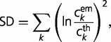
  by minimizing the square log deviation (SLD) in log space
 |
(3) |
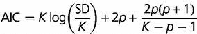
over the parameters of the model and using the corrected AIC (Akaike 1974) to differentiate between models with differing numbers p of parameters
 |
(4) |
Population Model with Additive Fitness
Models A, B, and C postulate parametrized gene replacement rate distributions. A more plausible and perhaps more realistic distribution should emerge from a stochastic population model with selection in which gene loss and acquisition are modeled explicitly. Below we describe such a model and derive the steady-state distribution of gene replacement rates analytically.
Consider a population of N individuals each harboring M genes. Each gene has a fixed additive contribution f to the organism’s fitness. Selection and drift are implemented via a Moran process (Moran 1962). At every iteration of the process, the progeny of the selected individual is subjected to a mutation process in which every gene is replaced with mutation probability V. The fitness effect of the new gene is drawn from an exponential distribution with a unit mean (Gillespie 1984). This distribution is chosen arbitrarily. However, it is generic, parameter free, and produces genes with a broad range of fitness contributions. It remains to be explored how the shape of the new gene fitness distribution affects the steady-state distribution of turnover rates.
In the weak mutation limit  , mutations appear sequentially and are either fixed or purged before the next mutation occurs. Then the distribution
  of fitness effects obeys an evolution equation
| (5) |
where L(f ) is the loss rate and G(f ) is the gain rate of a gene with fitness effect f
| (6) |
 |
(7) |
Here,  is the total fitness of the wild-type organism,
  is the rate of appearance of new genes and
  is the probability of fixation of an organism of fitness
  which appears in a population of size N in which all other organisms have fitness s. For the Moran process (Moran 1962),
| (8) |
Because the fitness contributions of new genes is drawn from an exponential distribution with unit mean, the characteristic fitness on an organism in steady state is  , the genome size. Similarly, the characteristic change in fitness due to a mutation is of order unity. Therefore, the factor
  in equation (8) is different from unity by approximately
  . Because
  is raised to the power N in the denominator of equation (8), the ratio N/M of the population size to the genome size determines the strength of selection. When
  , the fixation probability
  depends weakly on the fitness gain or loss and thus selection is weak. Conversely, in the strong selection limit
  , deleterious mutations are always purged, and beneficial mutations of moderate advantage (
 ) are always fixed.
In steady state, the distribution of fitness effects  is independent of time and is found by solving the nonlinear integral equation
  in conjunction with equations (6–8). We transform the integral equation to a system of nonlinear algebraic equations by discretizing f and
  and solving the resulting system using the Levenberg–Marquardt method (Marquardt 1963).
The distribution of fitness effects  can be converted to the steady-state distribution
  of gene replacement rates by noting that the loss rate in equation (6) is actually the replacement rate
  . Because the relationship between L and f is monotonic, it can be inverted
  . Using the conservation of probabilities we obtain
| (9) |
When selection is weak, that is, when  , the distribution of replacement rates is peaked at the maximum rate, which is approximately
  (see supplementary fig. S4, Supplementary Material online). In the limit of strong selection (
 ), the distribution approaches
  , so that each decade in rate contributes an equal weight to the distribution.
Results
Models of Genome Evolution
In the SGT framework, organisms evolve along a tree, and their genome size is fixed. We justify this assumption by exploring a stochastic population model with gene deletion and innovation (see supplementary information, Supplementary Material online), which indicated that the genome size fluctuations are small for a broad range of parameters. The genes are placed to genomic slots each with an associated turnover rate. When a gene is turned over in a slot, it is replaced by a gene with a novel identity. In this respect, the SGT is similar to the IMG. The genomic slots can have an arbitrary distribution of turnover rates. We investigated four models of evolution within the SGT framework. In the neutral model (model A), nothing differentiates the genes, and all slots have the same turnover rate, that is, the distribution of turnover rates is a delta function. When selection is important and the intrinsic gene deletion rate is uniform among all genes, genes that confer a greater fitness advantage are lost from the population at a lower rate. Therefore, the models in which slots turn over at different rates are labeled as models with selection in this study. In the two-parameter model B, the rates are gamma distributed. The scale parameter of the Gamma distribution sets the overall evolutionary rate, whereas the shape parameter controls the strength of selection. A large shape parameter results in a sharply peaked distribution of turnover rates and therefore signifies weak selection. In model C, just as in Collins and Higgs (2012), there are two classes of genes: slow and fast evolving. Thus, model C has three fitting parameters: the rates of replacement for the slow-evolving genes and fast-evolving genes and the fraction of the genome that is assigned to the slowly evolving genes. Unlike models A, B, and C, in which the distribution of turnover rates is parametrized, in model D, this distribution derives from a stochastic population model described in detail in the Materials and Methods section. Model D has two parameters: first, the ratio of population size to the genome size, which reflects the strength of selection, and second, the rate of evolution.
The models were tested on a data set comprised approximately 400 groups of 10 prokaryotes spanning a wide range of evolutionary distances (see Materials and Methods for the details of the group formation). The empirical gene frequency distribution was computed for each group (see Materials and Methods for details), the frequency distributions derived from each of the four models were fit to each of the empirical distributions, and the goodness of fit was compared using the Akaike Information Criterion (AIC) (see Materials and Methods). Because the data set includes the total of 784 species, there were significant overlaps between the groups. Although the different groups were generally not independent from each other, the conclusions reached for the complete data set did not change qualitatively when the analysis was repeated with a reduced data set, which contained 17 nonoverlapping groups of closely related species (see supplementary information, Supplementary Material online).
Fit of Evolutionary Models to the Empirical Gene Frequency Distributions
Before discussing the fitting of the models to the data, we examine the variation of the empirical gene frequencies with evolutionary divergence. Figure 1 shows the frequencies c1 of unique and c10 of strictly common genes as a function of the mean tip to root branch length. Each point in figure 1 corresponds to one of the 400 groups or species. Predictably, the frequency of unique genes increases, whereas the frequency of common genes drops with the evolutionary distance; both dependencies are roughly linear. Notably, however, the frequency of common genes does not approach unity as the mean evolutionary distance tends to zero. It appears that different isolates of the same species (or even strain) can have as little as 70% of the genes in common. This observation reflects the known fact that closely related bacterial isolates can differ by as much as 30% of their gene sets, in particular due to acquisition of pathogenicity islands (Perna et al. 2001; Kudva et al. 2002; Zhang et al. 2007).
Fig. 1.—
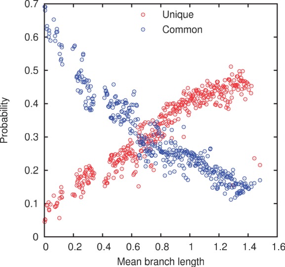
Probabilities c1 of encountering a unique gene and c10 of encountering a strictly common gene.
The gene frequency distributions produced by each of the four models were fit to the empirical distributions using a procedure described in the Materials and Methods. Figure 2 shows the gene frequency distributions and the corresponding model fits for four representative groups of prokaryotes spanning the range of evolutionary divergence analyzed in this work. Clearly, the neutral model (A) yields a substantially inferior fit to the observed gene frequencies compared to the models with selection. The distinction between the models is qualitative rather than only quantitative: unlike each of the models with selection, the neutral models fails to reproduce the U-shaped distribution yielding instead a peak at one of the intermediate gene frequency classes (fig. 2). A quantitative comparison of the fits using in the AIC shows that the difference between the models with selection and the neutral model is highly statistically significant (fig. 3 and table 1). The likelihood that model B fits the data better than model A, for example, is the exponential of the half of the difference in the respective AICs (Akaike 1974), that is, a difference of 10 in the AIC translates to a P value of  . The three models with selection differed from each other much less than each of them differed from the neutral model, but, nevertheless, model D on average yielded a significantly better fit that models B and C (fig. 3 and table 1).
Fig. 2.—

Gene frequency distributions and model fits for four groups of bacteria. The underlying trees and the mean branch lengths are shown in the insets.
Fig. 3.—
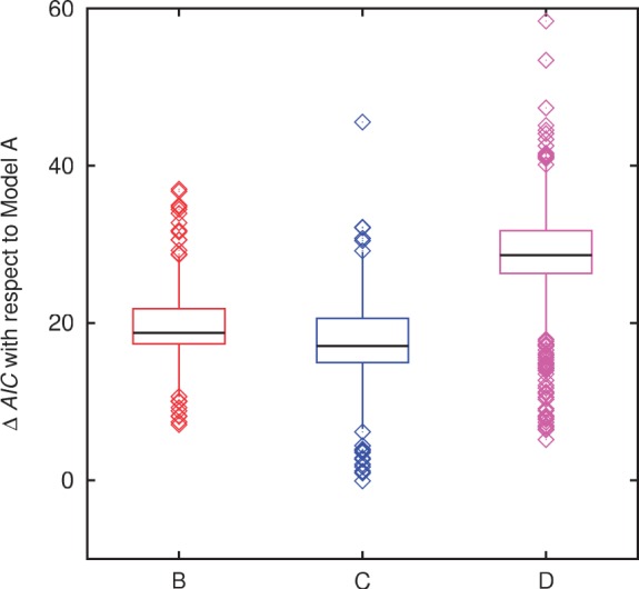
Summary of the distributions of the AIC differences between the models with selection and the neutral model across all 400 analyzed groups of prokaryotes.
Table 1.
P values for the Neutral Model A to Provide a Better Fit than the Three Models with Selection for the Groups Shown in Figure 2
| Group | Branch Length | Model B | Model C | Model D |
|---|---|---|---|---|
| 23 | 0.205 |  |
 |
 |
| 94 | 0.506 |  |
 |
 |
| 184 | 0.784 |  |
 |
 |
| 312 | 1.168 |  |
 |
 |
| Average over all groups |  |
 |
 |
|
Note:—The bottom line shows the geometric mean of the P values among all groups.
Each of the three models with selection included a parameter that reflected selection strength: the inverse shape parameter in model B, the fraction of slowly evolving genes in model C, and the ratio of the population size to the genome size in model D (see Materials and Methods for details). The replacement rate distributions in models B and D are more sharply peaked when selection is weaker. In model C, selection strength is reflected in the fraction of the genome that evolves under stronger selection and therefore has a lower replacement rate. Figure 4 shows the dependence of the estimated selection strength on the evolutionary distance. Perhaps counterintuitively, the selection pressure consistently and sharply declines with divergence under each of the three models. The selection pressure translates into the breadth of the distribution of the gene turnover rates. Weaker selection implies a more peaked distribution of turnover rates with diminished contributions from both the high and the low turnover rates. The dearth of high turnover rates at longer evolutionary distances may be explained by the fact that multiple turnovers in the same slot on the same branch of a tree are undetectable. Thus, the highest detectable turnover rate is set by the shortest branch in the tree. Conversely, for groups of closely related organisms, there might have not been enough time to experience replacements of many genes. The weight of the low turnover rate tail of the distribution may therefore be overestimated in closely related groups. These two factors that probably lead to the observed decrease in the contribution of selection to the observed gene frequency distributions with evolutionary distance effectively stem from the simplifying assumptions of the employed models of evolution (made to ensure model tractability). However, it is also possible that with the increasing divergence of genomes, gene replacements increasingly involve metabolic, signal transduction, and other gene modules, so that selection becomes relevant only for the conservation of the core genes that largely encode components of information processing systems.
Fig. 4.—
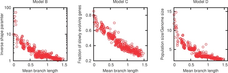
Dependence of the selection strength estimated from the fits of models B, C, and D to the empirical gene frequency distributions on the mean branch length in the phylogenetic tree.
All models include a parameter that reflects the characteristic gene replacement rate. If the gene repertoires of prokaryotes are shaped by the same mechanisms throughout the range of evolutionary divergences and if the SGT model captures these mechanisms, the gene turnover rate should be independent of the mean branch length from tip to root. Figure 5 shows the estimated turnover rates in model C (the evolutionary rate parameter in other models tracks that of model C closely up to a multiplicative factor) measured in gene turnovers per substitution-per-site. The rates are roughly independent of the mean branch length for moderate to large divergences. The slowly evolving genes are replaced on average once for every 10 substitutions per site, whereas the quickly evolving genes turn over when a single substitution per site on average has been accumulated. The sharp increase in the estimated rates at the shortest evolutionary distance apparently indicates that some of the SGT assumptions break down in this distance range. A possible explanation for the spike in the estimated evolutionary rate might be the greater contribution of gene transfer processes that affect multiple genes at a time, such as transfer of pathogenicity and symbiosis islands at short evolutionary distances (Groisman and Ochman 1996; Juhas et al. 2009).
Fig. 5.—
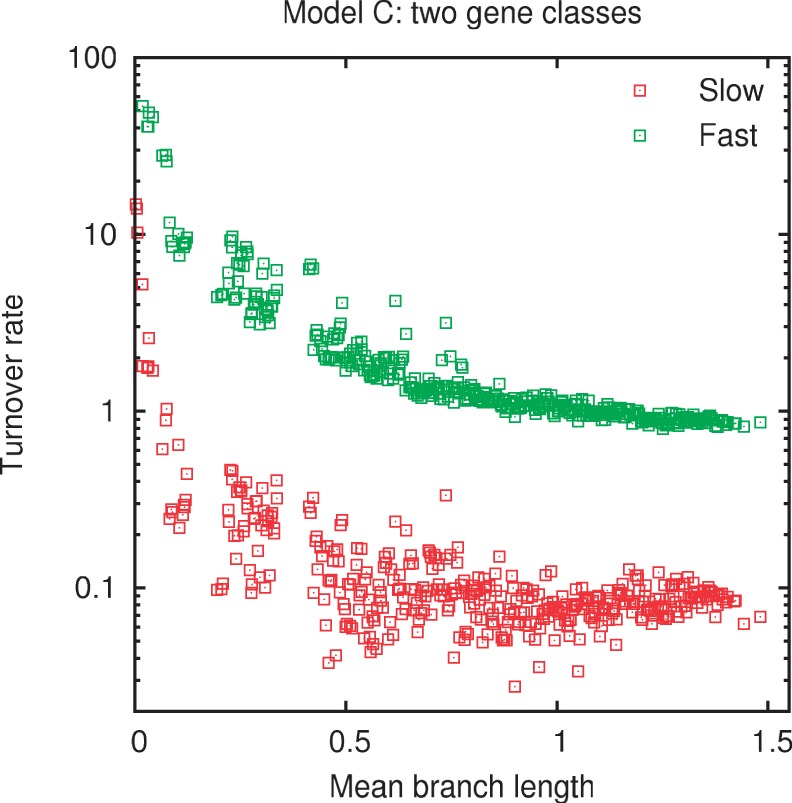
The gene turnover rates estimated from the fits of the two-class model C to the empirical gene frequency distributions.
Discussion
The nontrivial, asymmetrical U-shape of the gene frequency distribution that is observed in prokaryotic pangenomes through a broad range of phylogenetic depths calls for an explanation that arguably would come in the form of a maximally realistic yet tractable model of evolution. Evolutionary genomics and evolutionary systems biology yielded universal distributions of several biologically important quantities and attempts have been made to explain (that is reproduce) these distributions via models of evolution that are either neutral or include various forms of selection (Koonin 2011a). For example, the power law distribution of the size of paralogous families that has essentially the same shape for all available genomes is well approximated with birth–death innovation without selection (Huynen and van Nimwegen 1998; Karev et al. 2002; Koonin et al. 2002). Similar nonadaptive models have been invoked to explain the evolution of genetic networks (Lynch 2007b). In contrast, the universal log-normal distribution of evolutionary rates of orthologous genes seems to require purifying selection as an intrinsic component of the underlying evolutionary model (Lobkovsky et al. 2010). A recent study has suggested that a neutral model might be sufficient to explain the U-shape of the gene frequency distribution (Collins and Higgs 2012), whereas an analysis based on a different underlying model led to the rejection of the neutral model (Baumdicker et al. 2012). Each of these analyses involved a small sample of bacteria and required a moderately large number of parameters for a reasonable fit putting the generality of the conclusions into question.
We sought to investigate whether selection is required to explain the observed shape of the gene frequency distributions by analyzing a large sample of bacterial and archaeal groups that span a wide range of evolutionary divergence. To model genome evolution, we developed the SGT framework. The key assumption of the SGT is that the genome is in steady state throughout evolution. This assumption translates in practice into the fixed genome size and distribution of gene turnover rates. The fixed genome size assumption is certainly a simplification but, given the relatively narrow, sharply peaked distributions of bacterial and archaeal genome sizes (Koonin and Wolf 2008; Koonin 2011b), assuming stationary genomes on the evolutionary scale appears to be realistic. In addition, the results of a stochastic population model with gene duplication and deletion suggest that the genome size fluctuations are small in a broad parameter range.
The SGT framework is flexible because it admits an arbitrary distribution of gene replacement rates. The breadth of this distribution reflects the selection pressure that constrains the underlying evolutionary processes ultimately responsible for gene turnover. We compared the fits of the empirical gene frequency distributions for 400 groups of bacteria and archaea to the neutral model, in which all genes have the same turnover rate, to the fits produced by three other models with selection. The goodness of fit measured by the AIC indicates that the neutral model does not account for the observed gene frequency histograms nearly as well as the models with selection. Moreover, the difference between the neutral model and the models that incorporate selection is qualitative: the neutral model fails to mimic the U-shaped gene frequency distribution yielding no core of highly conserved genes. Among the three examined models with selection, the best fit on average resulted from using the distribution of gene turnover rates produced by stochastic population dynamics with additive per-gene fitness effects in which the fixation of mutant genes was considered explicitly. Although this model is the most complicated and arguably most realistic of the three models with selection, it is still oversimplified (even apart from the general SGT assumptions) because it ignores intergenic epistasis, undoubtedly an important aspect of evolution (Phillips 2008). A more detailed examination of the model D fit to the empirical gene frequency distributions shows that the model systematically overestimates the fraction of rare genes and underestimates the fraction of the common genes (fig. 6). This effect could result from the underestimation of the selection strength. The positive intergenic epistasis ignored by the additive fitness assumption could render the selective coefficient for a group of genes greater than the sum of the selective coefficients of the constituent individual genes.
Fig. 6.—

The fit of the stochastic model D to the empirical gene frequency histogram: the residuals for gene commonality classes among all groups.
The model fits yield information about the effective selection pressure that is responsible for the observed gene frequency distribution. We found a sharp decline of the selection strength with evolutionary distance, which manifested in the sharper peaked, more narrow distributions of replacement rates for groups of organisms with high mean divergence. We suggest that narrowing of the estimated distribution of replacement rates—and accordingly diminished selection with divergence—is at least in part due to two limitations of comparative genome analysis. First, the weight of low replacement rates is overestimated in closely related groups and second, the high replacement rates cannot be measured in divergent groups. However, these limitations notwithstanding, it cannot be ruled out that at large evolutionary distances, when entire gene modules are replaced in the compared organisms, selection is evident only for small cores of highly conserved, essential genes, primarily those involved in genomic information processing.
Fitting the gene frequencies in model D to the empirical gene frequencies yields estimates of the ratios of the population size to the genome size. The best fits translate to effective population sizes of  . The population sizes that are measured for bacteria typically are at least an order of magnitude larger (Lynch 2006). However, the small effective population size that emerges as the best fit in our models of genome evolution might reflect the substantial evolutionary effect of population bottlenecks (Lynch 2007a).
The characteristic rate of evolution yielded by the explored models with selection is roughly constant over a large portion of the range of evolutionary divergence. This observation implies that the SGT assumptions could be reasonable in that range. However, the extracted rates of evolution exhibit a large spike at short evolutionary distances, possibly due to horizontal transfer of large genomic segments including many genes. For this range of evolutionary distances, a modified approach to evolutionary modeling is probably required.
The main conclusion of this work is that selection made a substantial contribution to the mechanisms that shaped the universal gene frequency distribution in prokaryotes. Certainly, it would be unreasonable to question the existence of selection affecting genes responsible for key biological functions. However, it was far from obvious whether the effect of selection and its strength could be detected and measured at the level of the overall frequency distribution, without turning to individual genes. We believe that the present results solve this problem by demonstrating that a neutral model fails to explain the existence of the conserved gene core and moreover that models with different implementations of selection could be readily distinguished.
Supplementary Material
Supplementary information, table S1, and figures S1–S5 are available at Genome Biology and Evolution online (http://www.gbe.oxfordjournals.org/).
Literature Cited
- Akaike H. New look at statistical-model identification. IEEE Trans Automat Control. AC. 1974;19(6):716–723. [Google Scholar]
- Akopyants NS, et al. PCR-based subtractive hybridization and differences in gene content among strains of Helicobacter pylori. Proc Natl Acad Sci U S A. 1998;95(22):13108–13113. doi: 10.1073/pnas.95.22.13108. [DOI] [PMC free article] [PubMed] [Google Scholar]
- Altschul SF, et al. Gapped BLAST and PSI-BLAST: a new generation of protein database search programs. Nucleic Acids Res. 1997;25(17):3389–3402. doi: 10.1093/nar/25.17.3389. [DOI] [PMC free article] [PubMed] [Google Scholar]
- Baumdicker F, Hess WR, Pfaffelhuber P. The diversity of a distributed genome in bacterial populations. Ann Appl Probab. 2010;20(5):1567–1606. [Google Scholar]
- Baumdicker F, Hess WR, Pfaffelhuber P. The infinitely many genes model for the distributed genome of bacteria. Genome Biol Evol. 2012;4(4):443–456. doi: 10.1093/gbe/evs016. [DOI] [PMC free article] [PubMed] [Google Scholar]
- Charlebois RL, Doolittle WF. Computing prokaryotic gene ubiquity: rescuing the core from extinction. Genome Res. 2004;14(12):2469–2477. doi: 10.1101/gr.3024704. [DOI] [PMC free article] [PubMed] [Google Scholar]
- Collins RE, Higgs PG. Testing the infinitely many genes model for the evolution of the bacterial core genome and pangenome. Mol Biol Evol. 2012;4(4):443–465. doi: 10.1093/molbev/mss163. [DOI] [PubMed] [Google Scholar]
- Dagan T, Artzy-Randrup Y, Martin W. Modular networks and cumulative impact of lateral transfer in prokaryote genome evolution. Proc Natl Acad Sci U S A. 2008;105(29):10039–10044. doi: 10.1073/pnas.0800679105. [DOI] [PMC free article] [PubMed] [Google Scholar]
- Dehal PS, et al. MicrobesOnline: an integrated portal for comparative and functional genomics. Nucleic Acids Res. 2010;38(Database issue):396–400. doi: 10.1093/nar/gkp919. [DOI] [PMC free article] [PubMed] [Google Scholar]
- den Bakker HC, et al. Comparative genomics of the bacterial genus Listeria: genome evolution is characterized by limited gene acquisition and limited gene loss. BMC Genomics. 2010;11:688. doi: 10.1186/1471-2164-11-688. [DOI] [PMC free article] [PubMed] [Google Scholar]
- Gillespie JH. Molecular evolution over the mutational landscape. Evolution. 1984;38(5):1116–1129. doi: 10.1111/j.1558-5646.1984.tb00380.x. [DOI] [PubMed] [Google Scholar]
- Groisman EA, Ochman H. Pathogenicity islands: bacterial evolution in quantum leaps. Cell. 1996;87(5):791–794. doi: 10.1016/s0092-8674(00)81985-6. [DOI] [PubMed] [Google Scholar]
- Haegeman B, Weitz JS. A neutral theory of genome evolution and the frequency distribution of genes. BMC Genomics. 2012;13:196. doi: 10.1186/1471-2164-13-196. [DOI] [PMC free article] [PubMed] [Google Scholar]
- Huynen MA, van Nimwegen E. The frequency distribution of gene family sizes in complete genomes. Mol Biol Evol. 1998;15(5):583–589. doi: 10.1093/oxfordjournals.molbev.a025959. [DOI] [PubMed] [Google Scholar]
- Ishmael N, et al. Extensive genomic diversity of closely related Wolbachia strains. Microbiology. 2009;155(Pt 7):2211–2222. doi: 10.1099/mic.0.027581-0. [DOI] [PMC free article] [PubMed] [Google Scholar]
- Juhas M, et al. Genomic islands: tools of bacterial horizontal gene transfer and evolution. FEMS Microbiol Rev. 2009;33(2):376–393. doi: 10.1111/j.1574-6976.2008.00136.x. [DOI] [PMC free article] [PubMed] [Google Scholar]
- Karberg KA, Olsen GJ, Davis JJ. Similarity of genes horizontally acquired by Escherichia coli and Salmonella enterica is evidence of a supraspecies pangenome. Proc Natl Acad Sci U S A. 2011;108(50):20154–20159. doi: 10.1073/pnas.1109451108. [DOI] [PMC free article] [PubMed] [Google Scholar]
- Karev GP, Wolf YI, Rzhetsky AY, Berezovskaya FS, Koonin EV. Birth and death of protein domains: a simple model of evolution explains power law behavior. BMC Evol Biol. 2002;2:18. doi: 10.1186/1471-2148-2-18. [DOI] [PMC free article] [PubMed] [Google Scholar]
- Kettler GC, et al. Patterns and implications of gene gain and loss in the evolution of Prochlorococcus. PLoS Genet. 2007;3(12):e231. doi: 10.1371/journal.pgen.0030231. [DOI] [PMC free article] [PubMed] [Google Scholar]
- Koonin EV. Comparative genomics, minimal gene-sets and the last universal common ancestor. Nat Rev Microbiol. 2003;1(2):127–136. doi: 10.1038/nrmicro751. [DOI] [PubMed] [Google Scholar]
- Koonin EV. Are there laws of genome evolution? PLoS Comput Biol. 2011a;7(8):e1002173. doi: 10.1371/journal.pcbi.1002173. [DOI] [PMC free article] [PubMed] [Google Scholar]
- Koonin EV. 2011b. The logic of chance: the nature and origin of biological evolution. Chapter 3. FT Press Science Series. Upper Saddle River (NJ): Pearson Education. [Google Scholar]
- Koonin EV, Wolf YI. Genomics of bacteria and archaea: the emerging dynamic view of the prokaryotic world. Nucleic Acids Res. 2008;36(21):6688–6719. doi: 10.1093/nar/gkn668. [DOI] [PMC free article] [PubMed] [Google Scholar]
- Koonin EV, Wolf YI, Karev GP. The structure of the protein universe and genome evolution. Nature. 2002;420(6912):218–223. doi: 10.1038/nature01256. [DOI] [PubMed] [Google Scholar]
- Kudva IT, et al. Strains of Escherichia coli O157:H7 differ primarily by insertions or deletions, not single-nucleotide polymorphisms. J Bacteriol. 2002;184(7):1873–1879. doi: 10.1128/JB.184.7.1873-1879.2002. [DOI] [PMC free article] [PubMed] [Google Scholar]
- Kunin V, Ouzounis CA. The balance of driving forces during genome evolution in prokaryotes. Genome Res. 2003;13(7):1589–1594. doi: 10.1101/gr.1092603. [DOI] [PMC free article] [PubMed] [Google Scholar]
- Lawrence JG, Hendrickson H. Genome evolution in bacteria: order beneath chaos. Curr Opin Microbiol. 2005;8(5):572–578. doi: 10.1016/j.mib.2005.08.005. [DOI] [PubMed] [Google Scholar]
- Lobkovsky AE, Wolf YI, Koonin EV. Universal distribution of protein evolution rates as a consequence of protein folding physics. Proc Natl Acad Sci U S A. 2010;107(7):2983–2988. doi: 10.1073/pnas.0910445107. [DOI] [PMC free article] [PubMed] [Google Scholar]
- Lynch M. Streamlining and simplification of microbial genome architecture. Annu Rev Microbiol. 2006;60:327–349. doi: 10.1146/annurev.micro.60.080805.142300. [DOI] [PubMed] [Google Scholar]
- Lynch M. Sunderland (MA): Sinauer Associates; 2007a. The origins of genome architecture. [Google Scholar]
- Lynch M. The evolution of genetic networks by non-adaptive processes. Nat Rev Genet. 2007b;8(10):803–813. doi: 10.1038/nrg2192. [DOI] [PubMed] [Google Scholar]
- Marquardt DW. An algorithm for least-squares estimation of nonlinear parameters. J Soc Ind Appl Math. 1963;11(2):431–441. [Google Scholar]
- Medini D, Donati C, Tettelin H, Masignani V, Rappuoli R. The microbial pan-genome. Curr Opin Genet Dev. 2005;15(6):589–594. doi: 10.1016/j.gde.2005.09.006. [DOI] [PubMed] [Google Scholar]
- Medini D, et al. Microbiology in the post-genomic era. Nat Rev Microbiol. 2008;6(6):419–430. doi: 10.1038/nrmicro1901. [DOI] [PubMed] [Google Scholar]
- Mira A, Martin-Cuadrado AB, D’Auria G, Rodriguez-Valera F. The bacterial pan-genome: a new paradigm in microbiology. Int Microbiol. 2010;13(2):45–57. doi: 10.2436/20.1501.01.110. [DOI] [PubMed] [Google Scholar]
- Mirkin BG, Fenner TI, Galperin MY, Koonin EV. Algorithms for computing parsimonious evolutionary scenarios for genome evolution, the last universal common ancestor and dominance of horizontal gene transfer in the evolution of prokaryotes. BMC Evol Biol. 2003;3:2. doi: 10.1186/1471-2148-3-2. [DOI] [PMC free article] [PubMed] [Google Scholar]
- Moran PAP. The statistical processes of evolutionary theory. Oxford. 1962: Clarendon Press. [Google Scholar]
- Perna NT, et al. Genome sequence of enterohaemorrhagic Escherichia coli O157:H7. Nature. 2001;409(6819):529–533. doi: 10.1038/35054089. [DOI] [PubMed] [Google Scholar]
- Phillips PC. Epistasis—the essential role of gene interactions in the structure and evolution of genetic systems. Nat Rev Genet. 2008;9(11):855–867. doi: 10.1038/nrg2452. [DOI] [PMC free article] [PubMed] [Google Scholar]
- Puigbò P, Wolf YI, Koonin EV. Search for a “tree of life” in the thicket of the phylogenetic forest. J Biol. 2009;8(6):59. doi: 10.1186/jbiol159. [DOI] [PMC free article] [PubMed] [Google Scholar]
- Rasko DA, et al. The pangenome structure of Escherichia coli: comparative genomic analysis of E. coli commensal and pathogenic isolates. J Bacteriol. 2008;190(20):6881–6893. doi: 10.1128/JB.00619-08. [DOI] [PMC free article] [PubMed] [Google Scholar]
- Reno ML, Held NL, Fields CJ, Burke PV, Whitaker RJ. Biogeography of the Sulfolobus islandicus pan-genome. Proc Natl Acad Sci U S A. 2009;106(21):8605–8610. doi: 10.1073/pnas.0808945106. [DOI] [PMC free article] [PubMed] [Google Scholar]
- Snel B, Bork P, Huynen MA. Genomes in flux: the evolution of archaeal and proteobacterial gene content. Genome Res. 2002;12(1):17–25. doi: 10.1101/gr.176501. [DOI] [PubMed] [Google Scholar]
- Tettelin H, Riley D, Cattuto C, Medini D. Comparative genomics: the bacterial pan-genome. Curr Opin Microbiol. 2008;11(5):472–477. doi: 10.1016/j.mib.2008.09.006. [DOI] [PubMed] [Google Scholar]
- Tetz VV. The pangenome concept: a unifying view of genetic information. Med Sci Monit. 2005;11(7):Y24–Y29. [PubMed] [Google Scholar]
- Touchon M, et al. Organised genome dynamics in the Escherichia coli species results in highly diverse adaptive paths. PLoS Genet. 2009;5(1):e1000344. doi: 10.1371/journal.pgen.1000344. [DOI] [PMC free article] [PubMed] [Google Scholar]
- Zhang Y, et al. Genome evolution in major Escherichia coli O157:H7 lineages. BMC Genomics. 2007;8:121. doi: 10.1186/1471-2164-8-121. [DOI] [PMC free article] [PubMed] [Google Scholar]
Associated Data
This section collects any data citations, data availability statements, or supplementary materials included in this article.