Some sampling properties of common phase estimators

Abstract

The instantaneous phase of neural rhythms is important to many neuroscience related studies. In this short note, the statistical sampling properties of three instantaneous phase estimators commonly employed to analyze neuroscience data are shown to share common features allowing for an analytical investigation into their behaviour. These three phase estimators – the Hilbert, complex Morlet, and discrete Fourier transform – are each shown to maximize the likelihood of the data, assuming the observation of different neural signals. This connection, explored with the use of a geometric argument, is used to describe the bias and variance properties of each of the phase estimators, their temporal dependence, as well as the effect of model miss-specification. This analysis suggests how prior knowledge about a rhythmic signal can be used to improve the accuracy of phase estimates.

1 Introduction

Coordination of brain activity across spatial and temporal scales is essential to healthy brain function, (Quyen, 2011). Understanding the mechanisms supporting this coordination remains an active research area. Rhythmic neural activity has been proposed to support dynamic coordination of collective neural behavior and function (Buzsaki, 2006; Buzsáki and Draguhn, 2004; Gray et al., 1989; Schroeder and Lakatos, 2008; Varela et al., 2001). Although many measures exist to characterize neural rhythms (e.g., Pereda et al. (2005); Young and Eggermont (2009)), recent interest has focused on the phase of neural rhythms, (e.g., Quyen and Bragin (2007)). For example, phase synchronization has been proposed as a basic mechanism for integration of brain activity in studies such as Harris et al. (2003); Varela et al. (2001); Womelsdorf et al. (2007), and the phase of low frequency rhythms has been shown to modulate high frequency fluctuations (i.e., cross-frequency coupling) in Canolty et al. (2006); Canolty and Knight (2010); Cohen (2008); Lakatos et al. (2008); Tort et al. (2008).

This brief communication focuses upon three estimators of instantaneous rhythm phase. These estimators are the discrete Fourier transform (DFT) based estimator, an estimator employing the Hilbert transform, and a phase estimator using the complex Morlet wavelet. Studies employing the Hilbert transform based phase estimator to estimate the phase of neurological signals include Buzsaki et al. (2003); Canolty et al. (2006); Hentschke et al. (2007); Palva et al. (2005); Sirota et al. (2008); Tort et al. (2008). The complex Morlet phase estimator is used for the same purpose in studies such as Lakatos et al. (2005); Rizzuto et al. (2006, 2003); Rutishauser et al. (2010). The DFT phase estimator is classically treated in books, for e.g. (Kay, 1993, p. 33).

The relative performance of the DFT, Hilbert and complex Morlet phase estimators has been documented in the neuroscience literature. In Guevara et al. (2005), the effect of reference on phase estimators applied to electroencephalographic data is investigated and in Hurtado et al. (2003) the phase-locking value is introduced which uses an a priori phase estimate. In these works comparisons are made via simulation without explicitly exploring the effect of parameter choice upon estimator accuracy and the relative performance of phase estimators for data in general. In Aviyente et al. (2011) & Aviyente and Mutlu (2011) a phase estimator based upon a time-frequency distribution is compared to a wavelet phase estimator. In these latter papers the statistical data model associated with the DFT phase estimator is presented.

The accuracy of the Hilbert and complex Morlet phase estimators is compared using both simulated and recorded neural data in Quyen et al. (2001), with a focus on derivative measures of phase synchrony. It is found that little practical difference exists between the Hilbert and complex Morlet phase estimators; but, the effect of parameter choice, time series length, noise level, signal amplitude and signal morphology is not fully addressed and relevant analytic expressions are not provided. In Bruns (2004), phase estimator differences are explored through deterministic calculation and by an analysis of a recording obtained from a subdurally implanted electrode on the cortical surface of a patient with epilepsy. It is found that two phase estimators considered in this scenario, identical to the Hilbert and complex Morlet phase estimators considered within the current work, can each be computed as a convolution of the data with an oscillatory window function. Further, when the oscillatory window functions are specified to have similar effective bandwidths, it is found that the Hilbert and Morlet phase estimators yield similar phase estimates. Unlike these previous works, the current work considers each method as a projection from which insight into the sampling properties of these phase estimators can be analytically derived. In this framework, by explicitly introducing noise and considering signal morphology, phase estimate accuracy is shown to explicitly depend on the number of measurements, on the additive noise variance, on the amplitude of the signal envelope, and upon the dimension of a relevant subspace. Further, it is shown that each of the three phase estimators considered are associated with different a priori information regarding the signal type, and each of these three estimators performs best when the actual signal present conforms to the a priori information. Thus, this paper further quantifies the nature of phase estimate accuracy in the neurosciences providing both an analytical basis for further theoretical advance as well as suggesting the appropriate use of a priori neural signal knowledge when estimating the phase of a neurological rhythm.

In this short note, by an application of classical statistics and a geometrical connection, the DFT, Hilbert, and complex Morlet instantaneous phase estimators are shown to be related; a result consistent with results presented in Bruns (2004) and in Quyen et al. (2001). Each of the three discussed estimators are shown to be maximum likelihood estimators; each estimator maximizing the likelihood associated with a unique, “matched” statistical data model. Facilitated by geometry, asymptotic estimator variance is given for each of the estimators, as well as induced temporal dependencies. All three can be computed as projection operations, where each method has its own projection matrix. The distribution of the phase estimator is determined by the effect of the projection on a signal vector term and upon a noise vector term. The note ends with a discussion on the impact of the current work upon practical instantaneous phase estimation. To the best of the authors’ knowledge this work is the first paper in the neuroscience literature documenting analytical sampling properties of commonly employed estimators of instantaneous phase.

2 Phase Estimator Properties

In the following sections, it is shown that the three estimators of instantaneous phase, the DFT, Hilbert and complex Morlet wavelet phase estimators, are each maximum-likelihood estimators associated with specific data models (Section (3)). The results of this paper are summarized in Table (1). Each row of Table (1) describes a specific type of instantaneous phase estimator. The columns of each row, from left to right, specify the estimator, the signal model for which the estimator is least-squares optimal, the equation in the text defining the model matrix in the linear statistical model for which the phase estimator is maximum likelihood, the dimension, p, of the span of the columns of the model matrix, and the equivalent prior information that is incorporated into the associated data model. These results, in conjunction with the geometry described in Fig. (1), and the phase estimator probability density function Eqn. (18), describe the essence of this work.

Table 1.

Phase Estimator Summary

Estimator	Matching Signal	Model Matrix	Projected Dimension, p	Prior Information
DFT	α ei2πf0t	Eqn. (23)	1	Sinusoid at f0
Hilbert	${\displaystyle \sum _{\text{k}=1}^{\text{N}\times \text{BW}\times \mathrm{\Delta }}}{\alpha }_{\text{k}}{\text{e}}^{\text{i}2\pi {\text{f}}_{\text{k}}\text{t}}$	Eqn. (26)	N × BW × Δ	Frequency interval centered upon f0.
Complex Morlet	$\alpha {\text{e}}^{-\frac{1}{{\text{f}}_{\text{b}}}\frac{{(\text{t}-\text{b})}^2}{{\text{a}}^2}}{\text{e}}^{\text{i}2\pi {\text{f}}_0\text{t}}$	Eqn. (33)	1	Gaussian envelope at time, b, modulated to frequency f0.

Figure 1.

The j^th element of the MLE signal estimate, (ŝ_mle)_j, is decomposed in the complex plane into a sum of the random noise vector (n_p)_j = (P_Hn_a)_j with the actual complex signal vector, (s_a)_j, directed along the actual instantaneous phase angle (φ_s)_j. The noise vector is randomly oriented, and when the variance, var {(ŝ_mle)_j} is small relative to |(s_a)_j|², φ_n is approximately equal to $\frac{{\left[{({\mathbf{n}}_{\text{p}})}_{\text{j}}\right]}_{\perp }}{\left|{({\mathbf{s}}_{\text{a}})}_{\text{j}}\right|}$.

3 Classical Theory

The following sections review relevant theory from classical statistics adapted to the problem of instantaneous phase estimation. This material will be used to develop the sampling properties of the three phase estimators discussed in this work.

3.1 Statistical Linear Model

The three phase estimators discussed in this note – the DFT, Hilbert and complex Morlet phase estimators – all involve taking the complex angle of a complex valued time-series. As shown in Section (4), these estimators can be associated with differing signal models in a classical, linear statistical model of the analytic signal, d_a, of the observed data, d, for a specific frequency of interest f₀.¹ The analytic signal is a complex-valued representation of the data consisting of only positive frequency components. For real-valued measurements, the discrete Fourier transform of the data, d, is redundant, in that all information is contained within the non-negative frequencies. Because of this, the analytic signal of the data, d_a, is lossless, possessing all of the information contained within the original time-series of measurements. That is, the measured data, d is related to the analytic signal, d_a, as Kay (1993),

$$\mathbf{d}=2\text{Re}\{{\mathbf{d}}_{\text{a}}\},$$ (1)

where Re {x} denotes the real part of the complex variable x.² In this work, the analytic signal, d_a, of the observed data, d is modeled as,

$${\mathbf{d}}_{\text{a}}={\mathbf{s}}_{\text{a}}+{\mathbf{n}}_{\text{a}}.$$ (2)

Here, s_a is the analytic signal representation of a rhythmic signal whose phase is to be estimated, and n_a is a zero-mean noise vector with Gaussian distributed and independent elements, each with variance σ². Relaxation of the Gaussian assumption is discussed in Section (6). Each of the phase estimators considered in this work correspond to maximum likelihood estimators associated with unique models of the signal s_a. The generic phase estimator, φ̂ is the complex angle of the maximum-likelihood estimator of the signal, ŝ_a,

$$\widehat{\mathit{\phi }}=\angle \{{\widehat{\mathbf{s}}}_{\text{a}}\},$$ (3)

and thus is also a maximum-likelihood estimator of the instantaneous phase, φ, since the transform of a maximum likelihood estimator is itself a maximum likelihood estimator of the transformed quantity (Hogg et al., 2005, p. 316). Here φ̂ is a vector of instantaneous phase estimators, the j^th element is associated with the phase (φ)_j of the signal, (s)_j, evaluated at time-index j. It is useful to model this signal in a linear relationship with an unknown vector of parameters, α. That is,

$${\mathbf{s}}_{\text{a}}=\mathbf{H}\mathit{\alpha }.$$ (4)

Here the model matrix, H depends on the type of phase estimator - DFT (dft), Hilbert (h), or complex Morlet (cm) - and has N rows, corresponding to the length of the data, and a number of columns that depends on the type of phase estimator.

3.2 Maximum-Likelihood Estimation

As previously discussed, φ̂ is maximum-likelihood (ML) if ŝ_a is maximum likelihood. The ML estimator of s_a is constructed by first estimating its transform in the frequency domain. The log-likelihood, ℓ(α), corresponding to the DFT of Eqn. (2) after substituting Eqn. (4), is

$$\ell (\mathit{\alpha })=\frac{-1}{2{\sigma }^2}\times {\left(\stackrel{\sim }{\mathbf{d}}-{\mathbf{U}}^{†}\mathbf{H}\mathit{\alpha }\right)}^{†}\left(\stackrel{\sim }{\mathbf{d}}-{\mathbf{U}}^{†}\mathbf{H}\mathit{\alpha }\right),$$ (5)

where U is the Fourier matrix specified as,

$${(\mathbf{U})}_{\text{j},\text{k}}=\frac{{\text{e}}^{\text{i}2\pi {\text{f}}_{\text{k}}{\text{t}}_{\text{j}}}}{\sqrt{\text{N}}},\text{j},\text{k}=0,\dots \frac{\text{N}}{2}-1,$$ (6)

where d̃ denotes discrete Fourier transformation of d, ${\text{f}}_{\text{k}}=\frac{\text{k}}{\text{N}\mathrm{\Delta }}$, t_j = jΔ, and Δ is the sample period. Here, without loss of generality, N is specified to be an integer power of 2. The j^th time-index and the k^th Fourier frequency are represented in the j^th row and the k^th column of U. Thus specified, U^†d computes the DFT, d̃ of the vector random data, d evaluated at the frequencies, f_k, $\text{k}=0,\dots ,\frac{\text{N}}{2}-1$ and is equal to U^†d_a, due to the restriction of the computation to the non-negative frequencies. Here ^† denotes transpose conjugation. Since U is invertible, all information contained in d_a is contained in d̃; the operation is lossless.

Now,

$${\widehat{\mathit{\alpha }}}_{\text{mle}}={({\mathbf{H}}^{†}{\mathbf{UU}}^{†}\mathbf{H})}^{-1}{\mathbf{H}}^{†}\stackrel{\sim }{\mathbf{Ud}},$$ (7)

$$={({\mathbf{H}}^{†}\mathbf{H})}^{-1}{\mathbf{H}}^{†}{\mathbf{d}}_{\text{a}}.$$ (8)

Thus, the projection of the analytic signal of the data onto the space spanned by the columns of H yields the maximum-likelihood estimator, ŝ_mle.³

$${\widehat{\mathbf{s}}}_{\text{mle}}=\mathbf{H}{({\mathbf{H}}^{†}\mathbf{H})}^{-1}{\mathbf{H}}^{†}{\mathbf{d}}_{\text{a}},$$ (9)

$$={\mathbf{P}}_{\text{H}}{\mathbf{d}}_{\text{a}},$$ (10)

where P_H is the projection matrix projecting onto the space spanned by the columns of the model matrix H. Thus, as specified in Eqn. (10), the maximum liklihood estimator of s_a is the projection of d_a onto the span of the columns of H. The maximum liklihood estimator, φ̂ of φ is,

$${\widehat{\mathit{\phi }}}_{\text{mle}}={tan}^{-1}\left(\frac{Im\{{\widehat{\mathbf{s}}}_{\text{mle}}\}}{Re\{{\widehat{\mathbf{s}}}_{\text{mle}}\}}\right).$$ (11)

In Section (4), φ̂_mle will be shown to be equal to the DFT, Hilbert and complex Morlet phase estimators for suitable choices of the model matrix, H.

3.3 bias {ŝ_mle}

The bias of the signal estimator depends upon the range of the projection matrix, P_H, and hence upon the range, or the span, of the columns of H. That is, if s_a belongs to the range of H, then s_a can be represented by a linear combination of the columns of H, and P_Hs_a = s_a. Since the noise is zero mean, the projected noise is also zero mean and E {P_Hd_a} = s_a. When P_Hs_a 6 ≠ s_a, ŝ_mle is biased. This mathematical description can be summarized as follows: when the model matrix H is matched to the transformed signal, the signal estimator is unbiased.

3.4 The distribution of (n_p)_j

The projected noise n_p = P_Hn_a, at time-index j, is shown in Appendix A to be distributed,⁴

$${({\mathbf{n}}_{\text{p}})}_{\text{j}}~\mathcal{C}\mathcal{N}\left(\mathbf{0},\frac{\text{p}{\sigma }^2}{\text{N}}\right).$$ (12)

Here, p = tr {P_H}, where tr {X}, is the trace of the matrix X. The projection decomposes the variance of the noise, σ², into fluctuations occuring within the span of H and fluctuations occuring within the space orthogonal to the span of H. Projected noise variance grows linearly with the dimension, p, that is, with the number of columns of H, and hence with the number of model unknowns. The projection is a geometrical way to understand the effect of estimator complexity on inferred signal. As expected, projected noise variance decreases as one over the number of measurements, N, and increases with model complexity.

3.5 var {(φ̂_mle)_j}

The situation describing the phase estimator performance at time-index j is shown in Figure (1) for the situation when ŝ_mle is unbiased. In this figure, the circularly-symmetric Gaussian projected noise, n_p, at time-index j, adds to the signal vector, s, in the complex plane to form the estimated signal vector, ŝ_mle,

$${\widehat{\mathbf{s}}}_{\text{mle}}={\mathbf{P}}_{\text{H}}{\mathbf{d}}_{\text{a}},$$ (13)

$$={\mathbf{s}}_{\text{a}}+{\mathbf{n}}_{\text{p}}.$$ (14)

When the variance of the real and imaginary parts of the projected noise, n_p is small relative to signal magnitude, the small angle approximation is valid, (s_a)_j + [(n_p)_j]_|| ≈ (s_a)_j and the phase estimator, (φ̂_mle)_j equals,

$${\left({\widehat{\mathit{\phi }}}_{\text{mle}}\right)}_{\text{j}}={({\mathit{\phi }}_{\text{s}})}_{\text{j}}+{tan}^{-1}\left(\frac{\left[{({\mathbf{n}}_{\text{p}})}_{\text{j}}\right]}{{({\mathbf{s}}_{\text{a}})}_{\text{j}}+{[{({\mathbf{n}}_{\text{p}})}_{\text{j}}]}_{\parallel }}\right),$$ (15)

$$\approx {({\mathit{\phi }}_{\text{s}})}_{\text{j}}+\frac{{\left[{({\mathbf{n}}_{\text{p}})}_{\text{j}}\right]}_{\perp }}{\left|{({\mathbf{s}}_{\text{a}})}_{\text{j}}\right|},$$ (16)

$$\stackrel{\text{d}}{=}{({\mathit{\phi }}_{\text{s}})}_{\text{j}}+\frac{Re\left\{{({\mathbf{n}}_{\text{p}})}_{\text{j}}\right\}}{\left|{({\mathbf{s}}_{\text{a}})}_{\text{j}}\right|}.$$ (17)

The equality in Eqn. (17) is equality in probability distribution. It results by noting that the projected noise, (n_p)_j, is isotropic due to circular symmetry; any two orthogonal components of (n_p)_j in the complex plane have identical distributions.

Here (φ_s)_j is the actual, unknown phase at time index j. In this large instantaneous SNR regime the phase estimator is a linear function of a normally distributed random variable; it too is normally distributed.⁵ In particular,

$${\left({\widehat{\mathit{\phi }}}_{\text{mle}}\right)}_{\text{j}}~\mathcal{N}\left({({\mathit{\phi }}_{\text{s}})}_{\text{j}},\frac{\text{p}{\sigma }^2}{2\text{N}{\left|{({\mathbf{s}}_{\text{a}})}_{\text{j}}\right|}^2}\right).$$ (18)

This result is established formally in the situation of the DFT phase estimator in, again for example, Kay (1993). In this situation, p = 1 and |(s_a)_j| = a for j = 0, … , N − 1. Note, |(s_a)_j| in the expression for the variance of the phase estimator, (φ̂_mle)_j. The accuracy of phase estimation depends upon amplitude.

While Eqn. (18) is accurate when the small angle approximation is valid, note that this geometry provides the basis to explore low signal to noise ratio regimes. One expects Taylor expansions to be useful in this regard.

3.6 Model Miss-Specification

Model miss-specification occurs when ŝ_mle is biased. In this situation, Fig. (1), is modified in the following way. Instead of (s_a)_j adding to the noise vector (n_p)_j to form the signal estimator, (ŝ_mle)_j, the expected signal, (E {ŝ_mle})_j adds to the noise vector to produce the signal estimator, (ŝ_mle)_j. Due to this replacement, (φ_s)_j is replaced with some other angle, in general differing from the actual angle (φ_s)_j, and angle estimator bias may be introduced. Further, this bias reduces the signal amplitude within the column space of H. This reduction increases φ_n, which increases phase angle estimator variance. That is, the signal s_a, can be decomposed as a sum of the expected maximum likelihood estimator, E {Ŝ_mle} with an error vector, b, describing estimator bias,

$$\text{E}\{{\widehat{\mathbf{s}}}_{\text{mle}}\}={\mathbf{s}}_{\text{a}}+\mathbf{b}.$$ (19)

Let E {ŝ_mle} = s₀. Then,

$${\mathbf{s}}_{\text{a}}={\mathbf{s}}_0-\mathbf{b},$$ (20)

$$=\text{E}\{{\mathbf{P}}_{\text{H}}{\mathbf{d}}_{\text{a}}\}-\text{E}\{{\mathbf{P}}_{{\text{H}}_{\perp }}{\mathbf{d}}_{\text{a}}\},$$ (21)

where P_H⊥ is the projection matrix that projects orthogonal to the column space of H. Now, through orthogonality, the signal energy, E_s, can be decomposed into the sum of two non-negative terms,

$$\begin{array}{l}{\text{E}}_{\text{s}}={\mathbf{s}}_{\text{a}}^{†}{\mathbf{s}}_{\text{a}},\\ ={\mathbf{s}}_0^{†}{\mathbf{s}}_0+{\mathbf{b}}^{†}\mathbf{b}.\end{array}$$

The signal energy unaccounted for by the maximum likelihood estimator of s_a is due to that part of the signal, b, lying outside the column space of H. In essence, s_a in Fig. (1) is replaced by E {ŝ_a}, which on average has a magnitude less than that of s_a. Thus, model miss-specification reduces the average estimated signal energy and tends to increase the variance of (φ̂_mle)_j.

3.7 Temporal Dependence of φ̂_mle

Conditioned upon (ŝ_mle)_j, (φ̂_mle)_j is independent of (φ̂_mle)_k, for k ≠ j. Thus, it suffices to study the temporal dependence of ŝ_mle. As this quantity is multivariate Gaussian, dependency is quantified via the second central moment:

$$\begin{array}{l}cov\{{\widehat{\mathbf{s}}}_{\text{mle}}\}=\text{E}\left\{{\mathbf{P}}_{\text{H}}{\mathbf{n}}_{\text{a}}{\mathbf{n}}_{\text{a}}^{†}{\mathbf{P}}_{\text{H}}^{†}\right\},\\ ={\sigma }^2{\mathbf{P}}_{\text{H}}.\end{array}$$ (22)

Note that Eqn. (22) is a matrix with complex values describing the temporal dependency both temporally within the real and imaginary parts, as well as between the real and the imaginary components temporally. When H is sinusoidal, temporal dependence is periodic and long-range. When H is narrowband, temporal dependence will be inversely proportional to the bandwidth. When H has finite-support, then temporal dependence is limited to the domain of support.

4 Results

Given the general instantaneous phase estimator properties reviewed in Section (3), all that remains to establish the performance of the DFT, Hilbert and complex Morlet wavelet estimators is to equate their computation with a specific projection, P_H, and matching signal type. The results are summarized in Table (1).

4.1 DFT Phase Estimator

The DFT model is that of a pure sinusoid. The analytic signal of a pure sinusoid at time index, j, with phase φ₀ and frequency f₀ is e^i2πf₀t_j. Thus,

$${({\mathbf{H}}^{(\text{dft})})}_{\text{j}}={\text{e}}^{\text{i}2\pi {\text{f}}_0{\text{t}}_{\text{j}}}.$$ (23)

4.2 Hilbert Phase Estimator

The DFT model is a reduced rank version of the Hilbert model. The Hilbert transform phase estimator is computed in the following manner. First, the data is band-pass filtered about a frequency of interest to obtain, d_bp. Then, the band-pass filtered data is Hilbert transformed to obtain d_hbp and finally an analytic signal representation of the data is constructed,

$${\mathbf{d}}_{\text{abp}}={\mathbf{d}}_{\text{bp}}+\text{i}{\mathbf{d}}_{\text{hbp}}.$$ (24)

The instantaneous Hilbert phase estimator is then the complex angle of the analytic signal representation of the bandpass filtered data,

$${\widehat{\mathit{\phi }}}_{\text{h}}=\angle \{{\mathbf{d}}_{\text{abp}}\}.$$ (25)

In the Fourier domain the Hilbert transform introduces a 90° phase shift to the negative frequencies and a −90° phase shift to the positive frequencies Kay (1993). Hence, the multiplication by i in Eqn. (24) introduces an overall phase shift of 180° for the data components at negative frequencies and a zero degree phase shift for the data components at positive frequencies. The result is that the complex valued quantity, d_abp is zero for negative frequencies and twice the discrete Fourier transform of d_bp for positive frequencies. Thus, the combined effect on d_abp is, up to non-ideal band-pass filtering effects, the projection of the data d onto the space spanned by the complex exponentials at positive frequencies belonging to the pass-band of the band-pass filter. That is,

$${\mathbf{H}}^{(\text{H})}=\left(\begin{array}{ccc}⋮& & ⋮\\ {\text{e}}^{\text{i}2\pi {\text{f}}_{{\text{J}}_0}{\text{t}}_{\text{m}}}& \dots & {\text{e}}^{\text{i}2\pi {\text{f}}_{{\text{J}}_1}{\text{t}}_{\text{m}}}\\ ⋮& & ⋮\end{array}\right)$$ (26)

where f_J0 is the frequency at which the pass-band of frequencies begins, and f_J1 is the frequency at which the pass-band ends. Here p, the dimension of the projection range, is equal to the number of Fourier components in the pass-band of the band-pass filter. Thus,

$$\text{p}=\text{N}\times \text{BW}\times \mathrm{\Delta },$$ (27)

where BW is the pass-band interval width in Hz.

4.3 Complex Morlet Phase Estimator

The complex Morlet phase estimator is typically obtained for a specific scale parameter, a, shift parameter b, bandwidth parameter f_b and center frequency, f_c, as the complex angle of the wavelet coefficient, Ψ_a,b,fc,fb,

$${\mathrm{\Psi }}_{\text{a},\text{b},{\text{f}}_{\text{c}},{\text{f}}_{\text{b}}}(\text{d})={\int }_{-\infty }^{\infty }\text{d}({\text{t}}^{\prime }){\psi }^{\ast }(\frac{{\text{t}}^{\prime }-\text{b}}{\text{a}})\text{d}{\text{t}}^{\prime },$$ (28)

where d(t) is the ideal, continuous-time data and,

$${\psi }^{\ast }(\frac{\text{t}-\text{b}}{\text{a}})={\text{e}}^{-\frac{1}{{\text{f}}_{\text{b}}}\frac{{(\text{t}-\text{b})}^2}{{\text{a}}^2}}{\text{e}}^{\text{i}2\pi {\text{f}}_{\text{c}}\left(\frac{\text{t}-\text{b}}{\text{a}}\right)}.$$ (29)

In practice, the integral in Eqn. (28) is approximated from finite duration data consisting of samples of the continuous-time data d(t). Modeling the finite, sampled data in vector form as a realization of the random vector d, and approximating the integral in Eqn. (28) with a truncated Riemann sum, one obtains Ψ̃_a,b,fc,fb,

$${\stackrel{\sim }{\mathrm{\Psi }}}_{\text{a},\text{b},{\text{f}}_{\text{c}},{\text{f}}_{\text{b}}}(\mathbf{d})=\mathrm{\Delta }\sum _{\text{n}=0}^{\text{N}-1}{(\mathbf{d})}_{\text{n}}{\text{e}}^{-\frac{1}{{\text{f}}_{\text{b}}}\frac{{(\text{n}\mathrm{\Delta }-\text{b})}^2}{{\text{a}}^2}}{\text{e}}^{\text{i}2\pi {\text{f}}_{\text{c}}\left(\frac{\text{n}\mathrm{\Delta }-\text{b}}{\text{a}}\right)}.$$ (30)

Taking the complex angle yields an estimator for the instantaneous phase evaluated at time, b. ie.

$${\widehat{\phi }}_{\text{b}}^{(\text{cm})}=\angle \left\{{\stackrel{\sim }{\mathrm{\Psi }}}_{\text{a},\text{b},{\text{f}}_{\text{c}},{\text{f}}_{\text{b}}}(\mathbf{d})\right\},$$ (31)

$$=\angle \{{\mathbf{P}}_{\text{H}}\mathbf{d}\},$$ (32)

where in this case, H is a single column with m^th element equal to,

$${({\mathbf{H}}^{(\text{cm})})}_{\text{m}}={\text{e}}^{-\frac{1}{{\text{f}}_{\text{b}}}\frac{{(\text{m}\mathrm{\Delta }-\text{b})}^2}{{\text{a}}^2}}{\text{e}}^{\text{i}2\pi {\text{f}}_{\text{c}}\left(\frac{\text{m}\mathrm{\Delta }-\text{b}}{\text{a}}\right)}.$$ (33)

Note that in this situation, the projection matrix depends upon the time-index, b, and further, the projection introduces real-valued scalings that do not affect the estimated phase.

5 Simulation

The three instantaneous phase estimators, for the j^th time step, are compared in simulation. Each simulation involves 100 iterations in which synthetic data are created, and the phase of a signal estimated using the three phase estimators. These phase estimates are then used, in a kernel-smoothing procedure, to estimate the probability density functions for each of the three phase estimators. The estimated probability density functions, along with a representative time-series, are shown for two signals measured with additive white Gaussian noise (AWGN). In the first simulation the signal is a sinusoid and the resulting estimator probability density functions are shown in Fig. (2), top. In this case, the DFT phase estimator matches the signal and has the minimum column space dimension, p, of one. This estimator out-performs the other two phase estimators. Here the Hilbert estimator is using a narrow band of frequencies centred upon the actual sinusoid frequency; it suffers no bias, but has a slightly increased column space dimension, p, and performs nearly as well as the DFT based phase estimator. The complex Morlet phase estimator possesses a model column space dimension of 1; but, does not match the sinusoid and hence has a biased signal estimate resulting in increased phase estimator variance due to signal mismatch. Next, this simulation is repeated with differing sinusoid amplitudes but with the standard deviation of the additive noise held constant.⁶ The standard deviation of the resulting phase estimators is plotted as a function of sinusoid amplitude in the bottom of Fig. (2), along with the theoretical standard deviation obtained from Eqn. (18). The actual phase estimator standard deviations are larger than the theoretical standard deviation with a discrepancy that reduces with signal amplitude. This discrepancy is due to the fact that the small angle approximation, used to obtain an expression for φ_n in Fig. (1), underestimates the actual value.

Figure 2.

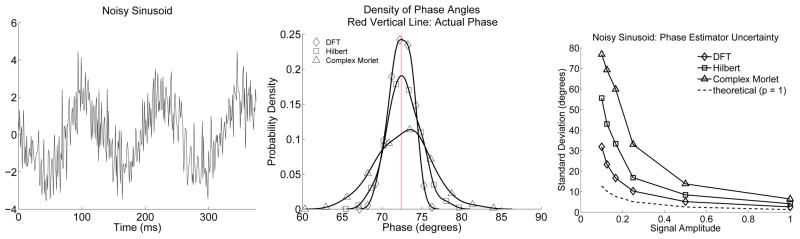
Left plot: A single realization of a sinusoid measured in AWGN. The signal to noise ratio (SNR) is 2, where here SNR is the average signal energy divided by average noise energy or, equivalently, divide by the noise variance. Middle plot: Probability density estimates at a specific time-index for the three instantaneous phase estimators, when used to estimate the phase of the sinusoid. Right plot: Phase estimator standard deviation plotted as a function of amplitude. The estimator employing the DFT has the least variance of the three phase estimators. The complex Morlet phase estimator uses a miss-specified model for this situation, and suffers increased variance and increased bias relative to the variance and bias of the other two phase estimators. The results are qualitatively consistent with theoretical developments, but note that the theoretical standard deviation (bottom plot) lower-bounds the realized standard deviation. This discrepancy decreases with sinusoid amplitude and results from the small angle approximation used to represent φ_n as $\frac{{\left[{({\mathbf{n}}_{\text{p}})}_{\text{j}}\right]}_{\perp }}{\mid {({\mathbf{s}}_{\text{a}})}_{\text{j}}\mid }$.

In the second simulation the signal is a broad-band pulse measured in AWGN. The resulting phase estimator densities are shown in Fig. (3). Now the performance ordering of the phase estimators is reversed. The Morlet estimator matches the signal, has a minimum model column space dimension, p, of 1, and outperforms the other phase estimators. The Hilbert estimator has less model mismatch than the DFT estimator, but pays for this better signal match in terms of column space dimension and only slightly out-performs the DFT estimator, which is mismatched to the broad-band pulse. Next, this simulation is repeated with differing pulse amplitudes but with the standard deviation of the additive noise held constant.¹ The standard deviation of the resulting phase estimators is plotted as a function of pulse amplitude in the bottom of Fig. (3), along with the theoretical standard deviation obtained from Eqn. (18). As in the first simulation, the actual phase estimator standard deviations are always larger than the theoretical standard deviation with a discrepancy that reduces with signal amplitude. Again, this discrepancy is due to the fact that the small angle approximation, used to obtain an expression for φ_n in Fig. (1), underestimates the actual value.

Figure 3.

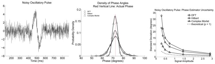
Left plot: A single realization of a Gaussian modulated pulse measured in AWGN. The signal to noise ratio is 0.84. Middle plot: Probability density estimates at a specific time-index for the three instantaneous phase estimators, when used to estimate the phase of a sinusoidally modulated Gaussian pulse. Right plot: Phase estimator standard deviation plotted as a function of pulse amplitude. The phase estimator based upon the DFT has the largest variance of the three phase estimators, consistent with the effect of model miss-specification. The complex Morlet phase estimator out-performs the other two estimators, owing to the fact that it uses a projection operator with a range of minimal dimension, while projecting the signal onto itself. The Hilbert phase estimator is not optimal, but rather suffers some model miss-specification and some increased variance due to the dimensionality of its assocatiated model matrix H^(H). The results are qualitatively consistent with theoretical developments, but note that the theoretical standard deviation (bottom plot) lower-bounds the realized standard deviation. This discrepancy decreases with pulse amplitude and results from the small angle approximation used to represent φ_n as $\frac{{\left[{({\mathbf{n}}_{\text{p}})}_{\text{j}}\right]}_{\perp }}{\mid {({\mathbf{s}}_{\text{a}})}_{\text{j}}\mid }$.

6 Discussion

The variance, bias and asymptotic distribution of the DFT, Hilbert transform based, and complex Morlet instantaneous phase estimators are established. Each of these estimators is shown to be a maximum likelihood estimator based upon a different signal model. Both the bias and variance are shown, in simulation and in theory, to depend upon the extent to which signal present in the data is matched to the phase estimator. The variance of each phase estimator is also shown to depend upon the complexity of the signal model to which it is associated; more complicated signal models yield models with a greater number of unknowns, and thus increased uncertainty, as described by the projection dimension, p; which is equal to the number of model unknowns. As represented in the right-most column in Table (1), estimator quality depends upon the quality of the information which its associated model embodies: if specific waveform shapes are known they can be used to form explicit phase estimators with a p of 1 and minimum variance, provided the actual signal matches the specified waveform. When model miss-specification occurs, a penalty is paid both in terms of bias and variance. This latter effect, due to a reduction in signal amplitude within the column space of the model matrix H, magnifies the effect of noise. On the other hand, increasing the model uncertainty, as in the Hilbert type estimator decreases susceptibility to model miss-specification; but, at the price of an increased p, and increased estimator variance.

In this work, the additive noise vector is assumed to be multivariate Gaussian and the elements of this vector are assumed to be uncorrelated; consistent with temporal independence. The assumption of Gaussianity is overly-restrictive since in the narrowband case (the case of interest), n_a, is dominated by a linear combination of a small number of DFT coefficients which are each asymptotically circularly-symmetric Gaussian without an a priori assumption of normality on the pre-Fourier transformed noise, see for example Walker (2000) and (Priestly, 1981, p. 466). The assumption of temporally uncorrelated noise, on the other hand, is important to the current results. If temporal correlation exists, then the real and imaginary parts of n_a for a given time index are correlated. When this occurs, the additive randomly oriented noise vector in Fig. (1), is no longer randomly oriented. One expects in this situation that estimators preferentially weighting time-indices where the additive noise vector is expected to lie parrallel to the signal will possess advantageous sampling properties.

The classical analysis presented in this paper provides an explicit relation governing the accuracy of commonly employed estimates of phase computed from noisy data. This relation, specifying both the effect of signal amplitude and the role of a priori signal knowledge on phase estimate accuracy, provides neuroscienctists with increased awareness when conducting phase based studies, as well as a basis for further understanding derivative quantities, such as measures of phase synchrony.

A The Distribution of (n_a)_j

The additive, complex valued noise vector, n_a in Eqn. (2) is equal to the analytic signal of the additive noise term, n, in the data model, d = s + n, where, for the sake of generality, E {n} = 0, and E {nn^T} = R is Toeplitz. In this case, the covariance between elements of the noise vector, n depends upon the absolute difference between element indices, consistent with a weak-sense stationary assumption. The analytic signal, n_a of the noise, n, is distributed mean-zero circularly-symmetric normal. This is shown by examining the moments of the real and imaginary parts of n_a, making use of the Fourier decomposition,

$${\mathbf{n}}_{\text{a}}=\sum _{\text{k}\in {\text{F}}_{+}}{\stackrel{\sim }{\mathbf{n}}}_{\text{k}}{\text{e}}^{\text{i}2\pi \frac{\text{kt}}{\text{N}}}.$$ (34)

Let ${\stackrel{\sim }{\text{n}}}_{\text{k}}^{(\text{r})}=Re\{{\stackrel{\sim }{\mathbf{n}}}_{\text{k}}\}$, and let ${\stackrel{\sim }{\text{n}}}_{\text{k}}^{(\text{i})}=Im\{{\stackrel{\sim }{\mathbf{n}}}_{\text{k}}\}$, denote the real and imaginary parts of the k^th element of ñ. Then,

$$\begin{array}{l}\text{E}\{Re\{{({\mathbf{n}}_{\text{a}})}_{\text{t}}\}Im\{{({\mathbf{n}}_{\text{a}})}_{{\text{t}}^{\prime }}\}\}=\frac{1}{\text{N}}\text{E}\left\{\sum _{\text{k},{\text{k}}^{\prime }\in {\text{F}}_{+}}Re\left\{{\stackrel{\sim }{\mathbf{n}}}_{\text{k}}{\text{e}}^{\text{i}2\pi \frac{\text{kt}}{\text{N}}}\right\}Im\left\{{\stackrel{\sim }{\mathbf{n}}}_{\text{k}}{\text{e}}^{\text{i}2\pi \frac{{\text{k}}^{\prime }{\text{t}}^{\prime }}{\text{N}}}\right\}\right\},\\ =\frac{1}{\text{N}}\text{E}\left\{\sum _{\text{k},{\text{k}}^{\prime }\in {\text{F}}_{+}}\left[{\text{n}}_{\text{k}}^{(\text{r})}cos2\pi \frac{\text{kt}}{\text{N}}-{\text{n}}_{\text{k}}^{(\text{i})}sin2\pi \frac{\text{kt}}{\text{N}}\right]\times \left[{\text{n}}_{\text{k}}^{(\text{r})}sin2\pi \frac{{\text{k}}^{\prime }{\text{t}}^{\prime }}{\text{N}}+{\text{n}}_{\text{k}}^{(\text{i})}cos2\pi \frac{{\text{k}}^{\prime }{\text{t}}^{\prime }}{\text{N}}\right]\right\},\\ =\frac{1}{\text{N}}\sum _{\text{k},{\text{k}}^{\prime }\in {\text{F}}_{+}}\text{E}\left\{{\text{n}}_{\text{k}}^{(\text{r})}{\text{n}}_{{\text{k}}^{\prime }}^{(\text{r})}\right\}cos2\pi \frac{\text{kt}}{\text{N}}sin2\pi \frac{{\text{k}}^{\prime }{\text{t}}^{\prime }}{\text{N}}-\text{E}\left\{{\text{n}}_{\text{k}}^{(\text{i})}{\text{n}}_{{\text{k}}^{\prime }}^{(\text{i})}\right\}cos2\pi \frac{\text{kt}}{\text{N}}sin2\pi \frac{{\text{k}}^{\prime }{\text{t}}^{\prime }}{\text{N}}.\end{array}$$ (35)

Here ${\text{F}}_{+}=\{\text{k}:0<\frac{\text{k}}{\text{N}}\le \frac{1}{2}\}$ is the set of positive frequencies, t, t′ are integer. Because $\text{E}\left\{{\text{n}}_{\text{k}}^{(\text{r})}{\text{n}}_{{\text{k}}^{\prime }}^{(\text{i})}\right\}$ is equal to zero due to circular symmetry for k, k′ ∈ F₊, terms involving $\text{E}\left\{{\text{n}}_{\text{k}}^{(\text{r})}{\text{n}}_{{\text{k}}^{\prime }}^{(\text{i})}\right\}$ do not contribute to Eqn. (35), and for clarity have been left out. Continuing,

$$\text{E}\left\{{\text{n}}_{\text{k}}^{(\text{r})}{\text{n}}_{{\text{k}}^{\prime }}^{(\text{r})}\right\}=\{\begin{array}{ccc}\frac{\text{S}({\text{f}}_{\text{k}})}{2}& ,& \text{k}={\text{k}}^{\prime },\text{k}\in {\text{F}}_{+}\\ 0& ,& \text{k}\ne {\text{k}}^{\prime }\end{array},$$ (36)

where S_n(f_k) is the spectrum of the additive noise, n, evaluated at frequency, ${\text{f}}_{\text{k}}=\frac{\text{k}}{\text{N}}$. When n has uncorrelated elements, S_n (f_k) is equal to σ² for k ∈ F₊. Note that without loss in generality, in this development the sample interval is taken to be 1. The spectrum requires scaling for the situation where the sample interval differs from 1 (so do the frequencies, but this scaling is cancelled by the time terms in the complex exponential).

$$\begin{array}{l}\text{E}\{Re\{{({\mathbf{n}}_{\text{a}})}_{\text{t}}\}Im\{{({\mathbf{n}}_{\text{a}})}_{{\text{t}}^{\prime }}\}\}=\frac{{\sigma }^2}{\text{N}}\sum _{\text{k}\in {\text{F}}_{+}}cos2\pi \frac{\text{kt}}{\text{N}}sin2\pi \frac{\text{k}{\text{t}}^{\prime }}{\text{N}}-cos2\pi \frac{\text{kt}}{\text{N}}sin2\pi \frac{\text{k}{\text{t}}^{\prime }}{\text{N}},\\ =0(\text{by}\text{orthogonality}),\end{array}$$ (37)

for t, t′ = 0, 1, … , N − 1. A similar argument yields,

$$\text{E}\{Re\{{({\mathbf{n}}_{\text{a}})}_{\text{t}}\}Re\{{({\mathbf{n}}_{\text{a}})}_{{\text{t}}^{\prime }}\}\}=\frac{1}{2\text{N}}\sum _{\text{k}\in {\text{F}}_{+}}\text{S}({\text{f}}_{\text{k}})cos2\pi \frac{\text{kt}}{\text{N}}cos2\pi \frac{\text{k}{\text{t}}^{\prime }}{\text{N}}+\text{S}({\text{f}}_{\text{k}})sin2\pi \frac{\text{kt}}{\text{N}}sin2\pi \frac{\text{k}{\text{t}}^{\prime }}{\text{N}}.$$ (38)

When the spectrum, S(f_k) is white,

$$\begin{array}{l}\text{E}\{Re\{{({\mathbf{n}}_{\text{a}})}_{\text{t}}\}Re\{{({\mathbf{n}}_{\text{a}})}_{{\text{t}}^{\prime }}\}\}=\{\begin{array}{cc}\frac{1}{2\text{N}}\sum _{\text{k}\in {\text{F}}_{+}}{\text{S}}_{\text{n}}({\text{f}}_{\text{k}})& \text{t}={\text{t}}^{\prime }\\ 0& \text{t}\ne {\text{t}}^{\prime }\end{array},\\ =\{\begin{array}{cc}\frac{{\sigma }^2}{2}& \text{t}={\text{t}}^{\prime }\\ 0& \text{t}\ne {\text{t}}^{\prime }\end{array}.\end{array}$$ (39)

Thus, when the additive noise vector, n_a in Eqn. (2) has independent elements, each element is circularly-symmetric Gaussian with real and imaginary components that are independent. Each of these components possess a variance equal to $\frac{{\sigma }^2}{2}$. With an application of Eqn. (37) and Eqn. (39), one obtains,

$$\text{E}\left\{{\mathbf{n}}_{\text{a}}{\mathbf{n}}_{\text{a}}^{†}\right\}={\sigma }^2\mathbf{I},$$ (40)

where I is the identity matrix. The variance of the projected noise, n_p = P_Hn_a, is computed as follows:

$$\begin{array}{l}\text{E}\left\{\sum _{\text{j}}{\mid {({\mathbf{n}}_{\mathbf{p}})}_{\text{j}}\mid }^2\right\}=\sum _{\text{j}}\text{E}\{{\mid {({\mathbf{n}}_{\mathbf{p}})}_{\text{j}}\mid }^2\},\\ \text{N}\text{E}\{{\mid {({\mathbf{n}}_{\mathbf{p}})}_{\text{j}}\mid }^2\}=\text{E}\{{{\mathbf{n}}_{\mathbf{p}}}^{†}{\mathbf{n}}_{\mathbf{p}}\},\\ \text{N}\text{E}\{{\mid {({\mathbf{n}}_{\mathbf{p}})}_{\text{j}}\mid }^2\}=\text{E}\left\{\text{trace}\left\{{\mathbf{P}}_{\mathbf{H}}{\text{n}}_{\text{a}}{\mathbf{n}}_{\text{a}}^{†}{\mathbf{P}}_{\text{H}}^{†}\right\}\right\},\\ \text{E}\{{\mid {({\mathbf{n}}_{\mathbf{p}})}_{\text{j}}\mid }^2\}=\frac{{\sigma }^2\text{trace}\{{\mathbf{P}}_{\mathbf{H}}\}}{\text{N}},\\ \text{E}\{{\mid {({\mathbf{n}}_{\mathbf{p}})}_{\text{j}}\mid }^2\}=\frac{\text{p}{\sigma }^2}{\text{N}}.\end{array}$$

Thus,

$$\begin{array}{l}\text{E}\{{\mid {({\mathbf{n}}_{\mathbf{p}})}_{\text{j}}\mid }^2\}=\text{E}{\{Re\{{({\mathbf{n}}_{\text{p}})}_{\text{j}}\}\}}^2+\text{E}{\{Im\{{({\mathbf{n}}_{\text{p}})}_{\text{j}}\}\}}^2,\\ =\frac{\text{p}{\sigma }^2}{\text{N}},\end{array}$$ (41)

implying,

$$\begin{array}{l}var\{Re\{{({\mathbf{n}}_{\text{p}})}_{\text{j}}\}\}=\frac{\text{p}{\sigma }^2}{2\text{N}},\\ =var\{Im\{{({\mathbf{n}}_{\text{p}})}_{\text{j}}\}\}.\end{array}$$ (42)

Thus, Eqn. (12) is established.

References

- Aviyente S, Bernat EM, Evans WS, Sponheim SR. A phase synchrony measure for quantifying dynamic functional integration in the brain. Human Brain Mapping. 2011;32 (1):80–93. doi: 10.1002/hbm.21000. [DOI] [PMC free article] [PubMed] [Google Scholar]
- Aviyente S, Mutlu A. A time-frequency-based approach to phase and phase synchrony estimation. Signal Processing, IEEE Transactions on. 2011 Jul;59 (7):3086–3098. [Google Scholar]
- Bruns A. Fourier-, hilbert-and wavelet-based signal analysis: are they really different approaches? Journal of neuroscience methods. 2004;137 (2):321–332. doi: 10.1016/j.jneumeth.2004.03.002. [DOI] [PubMed] [Google Scholar]
- Buzsaki G. Rhythms of the Brain. Oxford University Press; 2006. [Google Scholar]
- Buzsaki G, Buhl DL, Harris KD, Csicsvari J, Czeh B, Morozov A. Hippocampal network patterns of activity in a mouse. Neuroscience. 2003;116:201–211. doi: 10.1016/s0306-4522(02)00669-3. [DOI] [PubMed] [Google Scholar]
- Buzsáki G, Draguhn A. Neuronal oscillations in cortical networks. Science. 2004 Jun;304 (5679):1926–9. doi: 10.1126/science.1099745. [DOI] [PubMed] [Google Scholar]
- Canolty RT, Edwards E, Dalal SS, Soltani M, Nagarajan SS, Kirsch HE, Berger MS, Barbaro NM, Knight RT. High gamma power is phase-locked to theta oscillations in human neocortex. Science. 2006 Sep;313 (5793):1626–8. doi: 10.1126/science.1128115. [DOI] [PMC free article] [PubMed] [Google Scholar]
- Canolty RT, Knight RT. The functional role of cross-frequency coupling. Trends Cogn Sci (Regul Ed) 2010 Nov;14 (11):506–15. doi: 10.1016/j.tics.2010.09.001. [DOI] [PMC free article] [PubMed] [Google Scholar]
- Cohen MX. Assessing transient cross-frequency coupling in eeg data. J Neurosci Methods. 2008 Mar;168 (2):494–9. doi: 10.1016/j.jneumeth.2007.10.012. [DOI] [PubMed] [Google Scholar]
- Gray CM, König P, Engel AK, Singer W. Oscillatory responses in cat visual cortex exhibit inter-columnar synchronization which reflects global stimulus properties. Nature. 1989 Mar;338 (6213):334–7. doi: 10.1038/338334a0. [DOI] [PubMed] [Google Scholar]
- Guevara R, Velazquez J, Nenadovic V, Wennberg R, Senjanovi G, Dominguez L. Phase synchronization measurements using electroencephalographic recordings. Neuroinformatics. 2005;3(4):301–313. doi: 10.1385/NI:3:4:301. [DOI] [PubMed] [Google Scholar]
- Harris KD, Csicsvari J, Hirase H, Dragoi G, Buzsáki G. Organization of cell assemblies in the hippocampus. Nature. 2003 Jul;424 (6948):552–6. doi: 10.1038/nature01834. [DOI] [PubMed] [Google Scholar]
- Hentschke H, Perkins MG, Pearce RA, Banks MI. Muscarinic blockade weakens interaction of gamma with theta rhythms in mouse hippocampus. European Journal of Neuroscience. 2007;26:1642–1656. doi: 10.1111/j.1460-9568.2007.05779.x. [DOI] [PubMed] [Google Scholar]
- Hogg RV, McKean JW, Craig AT. Introduction to Mathematical Statistics. 6. Pearson Prentice Hall; 2005. [Google Scholar]
- Hurtado JM, Rubchinsky LL, Sigvardt KA. Statistical method for detection of phase-locking episodes in neural oscillations. Journal of Neurophysiology. 2003;91:1883–1898. doi: 10.1152/jn.00853.2003. [DOI] [PubMed] [Google Scholar]
- Kay SM. Fundamentals of Statistical Signal Processing: Estimation Theory. Prentice Hall PTR; Upper Saddle River, New Jersey: 1993. [Google Scholar]
- Lakatos P, Karmos G, Mehta AD, Ulbert I, Schroeder CE. Entrainment of neuronal oscillations as a mechanism of attentional selection. Science. 2008 Apr;320 (5872):110–3. doi: 10.1126/science.1154735. [DOI] [PubMed] [Google Scholar]
- Lakatos P, Shah AS, Knuth KH, Ulbert I, Karmos G, Schroeder CE. An oscillatory hierarchy controlling neuronal excitability and stimulus processing in the auditory cortex. Journal of Neurophysiology. 2005;94:1904–1911. doi: 10.1152/jn.00263.2005. [DOI] [PubMed] [Google Scholar]
- Palva JM, Palva S, Kaila K. Phase synchrony among neuronal oscillations in the human cortex. J Neurosci. 2005 Apr;25 (15):3962–72. doi: 10.1523/JNEUROSCI.4250-04.2005. [DOI] [PMC free article] [PubMed] [Google Scholar]
- Pereda E, Quiroga R, Bhattacharya J. Nonlinear multivariate analysis of neurophysiological signals. Progress in Neurobiology. 2005 Jan; doi: 10.1016/j.pneurobio.2005.10.003. [DOI] [PubMed] [Google Scholar]
- Priestly MB. Spectral Analysis and Time Series. Elsevier Academic Press; 1981. [Google Scholar]
- Quyen MLV. The brainweb of cross-scale interactions. New Ideas in Psychology. 2011;29 (2):57–63. [Google Scholar]
- Quyen MLV, Bragin A. Analysis of dynamic brain oscillations: methodological advances. Trends Neurosci. 2007 Jul;30 (7):365–73. doi: 10.1016/j.tins.2007.05.006. [DOI] [PubMed] [Google Scholar]
- Quyen MLV, Foucher J, Lachaux JP, Rodriguez E, Lutz A, Martinerie J, Varela FJ. Comparison of hilbert transform and wavelet methods for the analysis of neuronal synchrony. Journal of Neuroscience Methods. 2001;111 (2):83– 98. doi: 10.1016/s0165-0270(01)00372-7. [DOI] [PubMed] [Google Scholar]
- Rizzuto DS, Madsen JR, Bromfield E, Schulze-Bonhage A, Kahana MJ. Human neocortical oscillations exhibit theta phase differences between encoding and retrieval. NeuroImage. 2006;31:1352–1358. doi: 10.1016/j.neuroimage.2006.01.009. [DOI] [PubMed] [Google Scholar]
- Rizzuto DS, Madsen JR, Bromfield EB, Schulze-Bonhage A, Seelig D, Aschenbrenner-Scheibe R, Kahana MJ. Reset of human neocortical oscillations during a working memory task. Proceedings of the National Academy of Sciences, Neuroscience. 2003;100 (13):7931–7936. doi: 10.1073/pnas.0732061100. [DOI] [PMC free article] [PubMed] [Google Scholar]
- Rutishauser U, Ross IB, Mamelak AN, Schuman EM. Human memory strength is predicted by theta-frequency phase-locking of single neurons. Nature. 2010 Apr;464 (7290):903–7. doi: 10.1038/nature08860. [DOI] [PubMed] [Google Scholar]
- Scharf LL. Statistical Signal Processing: detection, estimation, and time series analysis. Addison-Wesley Publishing Company, Inc; 1991. [Google Scholar]
- Schroeder C, Lakatos P. Low-frequency neuronal oscillations as instruments of sensory selection. Trends Neurosci. 2008 Nov; doi: 10.1016/j.tins.2008.09.012. [DOI] [PMC free article] [PubMed] [Google Scholar]
- Sirota A, Montgomery S, Fujisawa S, Isomura Y, Zugaro M, Buzsaki G. Entrainment of neocortical neurons and gamma oscillations by the hippocampal theta rhythm. Neuron. 2008;60:683–697. doi: 10.1016/j.neuron.2008.09.014. [DOI] [PMC free article] [PubMed] [Google Scholar]
- Tort ABL, Kramer MA, Thorn C, Gibson DJ, Kubota Y, Graybiel AM, Kopell NJ. Dynamic cross-frequency couplings of local field potential oscillations in rat striatum and hippocampus during performance of a t-maze task. PROCEEDINGS OF THE NATIONAL ACADEMY OF SCIENCES OF THE UNITED STATES OF AMERICA. 2008 Dec;105 (51):20517–22. doi: 10.1073/pnas.0810524105. [DOI] [PMC free article] [PubMed] [Google Scholar]
- Tort ABL, Kramer MA, Thorn C, Gibson DJ, Kubota Y, Graybiel AM, Kopell NJ. Dynamic cross-frequency couplings of local field potential oscillations in rat striatum and hippocampus during performance of a t-maze task. Proceedings of the National Academy of Sciences of the United States of America. 2008;105(51) doi: 10.1073/pnas.0810524105. [DOI] [PMC free article] [PubMed] [Google Scholar]
- Varela F, Lachaux JP, Rodriguez E, Martinerie J. The brainweb: phase synchronization and large-scale integration. Nat Rev Neurosci. 2001 Apr;2 (4):229–39. doi: 10.1038/35067550. [DOI] [PubMed] [Google Scholar]
- Walker A. Some results concerning the asymptotic distribution of sample fourier transforms and periodograms for a discrete-time stationary process with a continuous spectrum. Journal of Time Series Analysis. 2000;21 (1):95–109. [Google Scholar]
- Womelsdorf T, Schoffelen JM, Oostenveld R, Singer W, Desimone R, Engel AK, Fries P. Modulation of neuronal interactions through neuronal synchronization. Science. 2007 Jun;316 (5831):1609–12. doi: 10.1126/science.1139597. [DOI] [PubMed] [Google Scholar]
- Young CK, Eggermont JJ. Coupling of mesoscopic brain oscillations: recent advances in analytical and theoretical perspectives. Prog Neurobiol. 2009 Sep;89 (1):61–78. doi: 10.1016/j.pneurobio.2009.06.002. [DOI] [PubMed] [Google Scholar]