The ‘39 steps’: an algorithm for performing statistical analysis of data on energy intake and expenditure

Abstract

The epidemics of obesity and diabetes have aroused great interest in the analysis of energy balance, with the use of organisms ranging from nematode worms to humans. Although generating energy-intake or -expenditure data is relatively straightforward, the most appropriate way to analyse the data has been an issue of contention for many decades. In the last few years, a consensus has been reached regarding the best methods for analysing such data. To facilitate using these best-practice methods, we present here an algorithm that provides a step-by-step guide for analysing energy-intake or -expenditure data. The algorithm can be used to analyse data from either humans or experimental animals, such as small mammals or invertebrates. It can be used in combination with any commercial statistics package; however, to assist with analysis, we have included detailed instructions for performing each step for three popular statistics packages (SPSS, MINITAB and R). We also provide interpretations of the results obtained at each step. We hope that this algorithm will assist in the statistically appropriate analysis of such data, a field in which there has been much confusion and some controversy.

Introduction

The twin epidemics of obesity and diabetes have placed a great premium on understanding more about the regulation of energy balance and how its dysregulation affects fat deposition and glucose homeostasis. Research in this area is being carried out using many organisms, including invertebrates such as Drosophila melanogaster and Caenorhabditis elegans, small mammals such as mice and rats, non-human primates, and humans. In particular, progress has been greatly facilitated by the generation of genetically manipulated animals (involving knockout, conditional knockout, knockdown, transgenic overexpression or optogenetic manipulation of targeted genes) in the last decade. Moreover, as our understanding of systems regulating energy balance improves, an increasing number of pharmaceutical and nutraceutical agents are being developed that aim to normalise energy balance.

The diversity of experimental approaches and organisms used to investigate energy balance calls for harmonisation in how data are analysed. This will mean that data derived using different approaches and organisms can be interpreted and compared with greater consistency. A particular concern in recent studies of small mammals has been how to normalise intake or expenditure data for differences in body mass or body composition of the animals (Arch et al., 2006; Butler and Kozak, 2010; Kaiyala and Schwartz, 2011; Tschöp et al., 2012). These issues are not new – the discussion of the optimal methods by which to normalise for body-mass effects began at least a century ago (Rubner, 1883; Kleiber, 1932; Kleiber, 1961). However, a consensus on this issue emerged in the 1990s in human studies. It was agreed that the best way forward was not to perform simple ratio calculations (e.g. expenditure divided by body mass, or lean body mass) because these approaches do not adequately normalise for the mass effect (Allison et al., 1995; Poehlman and Toth, 1995). Rather, the optimal approach is to correct for mass effects using a regression-based approach called analysis of covariance (ANCOVA) or general linear modelling (GLM). More recently, the same consensus has emerged among many researchers studying energy balance in small mammals (Kaiyala and Schwartz, 2011; Tschöp et al., 2012). Thus, a common framework for this analysis is now widely agreed on by researchers from the entire field, from those working with model organisms such as mice and flies, to those studying humans.

Despite this agreement of what should be done to analyse energy-balance data, researchers do not necessarily know how to do it. Therefore, the aim of this paper is to provide an algorithm as a step-by-step guide for performing this type of analysis. In an ideal world, the data generated from energy-balance experiments would be analysed with the help of a professional statistician. Our aim is not to replace that gold standard; if professional help is at hand then that will always be the best route for data analysis. However, access to professional statistical expertise is not always available. Indeed, two recent papers (Butler and Kozak, 2010; Tschöp et al., 2012) show that, in most cases, analyses of energy-balance data have been most frequently performed using approaches that would not be advised by a trained statistician, and that are at odds with the consensus that has been reached regarding analysis methods. Thus, we believe that a standardized algorithm that can be taken up by researchers throughout the field is of great importance. Even if professional help is at hand, researchers might find it useful to work through the analysis process before checking the outputs with a qualified statistician so as to better understand their own data.

The algorithm presented in this paper can be used in combination with any commercial statistics package. To assist with the analysis, we have provided the commands that should be used for three popular statistics packages (SPSS, MINITAB and R) in the supplementary material (supplementary material Appendices I, II and III, respectively). To use these commands, you simply go to the supplementary material Appendix for your preferred program, find the step in the algorithm you are at, and you will find details of the commands to use to run the analysis. We also provide with each supplementary material Appendix example outputs for the analysis, using example data we provide (see later), as well as guidance on how to interpret the outputs. Note that it is not possible to use this algorithm, or to correctly analyse this type of data, using packages designed principally to generate graphics or work as spreadsheets (such as PRISMGRAPH or Microsoft Excel) unless you perform complex programming to execute the appropriate tests. Because this requires specialist knowledge of the calculations involved in the statistical tests used, and how to program the packages, we strongly urge researchers to invest in statistical software that enables the analyses described. Note that, although we include the names of the statistical tests that are applied to the data, we do not detail the formulas on which the tests are based (beyond the scope of this manuscript). The formulas underlying the statistical tests used can be found in any advanced biostatistical textbook (e.g. Sokal and Rohlf, 2012; Zar, 2009). We cannot emphasise enough the importance of checking outputs with a qualified statistician before progressing to publication.

The data analysed using this algorithm should be of good quality, and involve a sufficiently large sample size. It is often assumed that sample sizes of six to ten individuals are adequate for this type of analysis, but studies based on such sample sizes are often underpowered (see e.g. Speakman, 2010). No level of statistical analysis can rescue poorly collected data or a dataset with a very small number of observations. The problem of having a small sample size is generally not resolved by combining the small sample with an inappropriate statistical analysis! Consulting a statistician before an experiment starts is useful for obtaining advice on a priori power analysis and sufficient sample sizes. In addition, advice on techniques and common pitfalls in available methods for measurements of food intake, energy expenditure and body composition can be found elsewhere (Lighton, 2008; Tschöp et al., 2012).

Preparing the data for analysis

Before using the algorithm, you should prepare the data and familiarise yourself with the terminology we use. We assume that a typical experiment involves measurements of either food intake [in grams or kg eaten, or kilojoules (kJ) or megajoules (MJ) of energy consumed in a given time period – usually a day] or energy expenditure [this can be expressed as oxygen consumption (e.g. ml of oxygen per minute or per hour), carbon dioxide production (ml of CO₂ per minute or per hour) or energy burned per unit of time (in watts, which are equivalent to joules per second, or expenditure over some other relevant time period, e.g. MJ/day or kJ/day)]. Note that mass does not feature in any of these units. In a typical experiment, these measurements will have been determined for several individuals, for which you will also have additional data, such as body mass and potentially body composition (e.g. fat mass, fat-free mass or even the masses of individual organs).

It is important to note that each individual should only appear in the dataset once in any given condition. It is not valid to include multiple data points for a single individual. For example, you might measure food intake every day for 10 days. The 10 separate days of data for a given individual are not ‘independent’ samples. All of the statistics mentioned in this algorithm assume the data being used are independent. In this example, if all the individuals have been measured in the same way, then you should use either the accumulated food intake over the entire 10 days or the mean over the 10 days – hence providing one independent data point per individual.

It is also important to note that data points should not be ‘normalised’ by dividing by body mass or lean body mass. Unfortunately, some of the equipment used to measure energy expenditure of animals (such as the CLAMS system) automatically makes this division before generating the final output data. To avoid this problem, we advise entering a body mass of 1.0 instead of the actual subject body mass when making measurements with this type of equipment. Alternatively, you can multiply output data from this type of equipment by body mass before proceeding.

The individuals that have been measured in your experiment can be divided into groups. This grouping reflects the treatment being performed. For example, the ‘treatment’ group could be animals deficient for a particular gene and the ‘control’ group would be animals with a wild-type genotype. A given experiment can have multiple treatments (e.g. multiple genotypes). Treatments can also have different ‘levels’. For example, the animals could be exposed to a drug thought to affect energy balance, and different animals could be given different doses of the drug. When using the algorithm, it is important to separate between different levels within a treatment, and different treatments. Homozygote and heterozygote animals for a particular gene should be treated as levels of a single treatment: they are effectively allele dosages.

Once the data are prepared, you should enter them into a statistical package to run the analysis. The three packages that we provide detailed instructions for are similar to most statistical packages in that all use a column-based operational structure. That is, comparisons and relationships are made between columns rather than between rows. For MINITAB and SPSS, data are entered into columns within the statistics package itself. In contrast, for R, datasets should be entered into a spreadsheet program (e.g. Microsoft Excel) and saved as tab-delimited .txt files. For all three packages, we suggest the following structure for data entry to analyse independent data:

• Column 1: subject ID (any alphanumeric code).

• Column 2: the data on food intake or energy expenditure. Recall that this must be the raw data, and should not be manipulated by dividing by mass or lean body mass.

• Column 3: the subject body mass.

• Column 4: the treatment group. Use a code such as C for control and T for treatment or any other alphanumeric code.

• Column 5: if appropriate, the different levels of the treatment. You can use numerical data here if referring to doses, or use an arbitrary alphanumerical code if levels are not doses.

• Column 6: data on lean body mass (if available).

• Column 7: data on fat mass (if available).

• Columns 8 onwards: other relevant data, such as masses of individual organs.

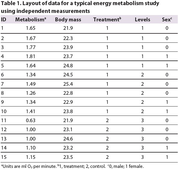
A typical dataset for this type of analysis is shown in Table 1. In this example, there are 15 individual animals in which metabolism and body mass were measured; animals were exposed to either a treatment (1) or control (2). The treatment had two levels. Note that the control is treated as a third level of the treatment in the column labelled ‘Levels’.

Table 1.

Layout of data for a typical energy metabolism study using independent measurements

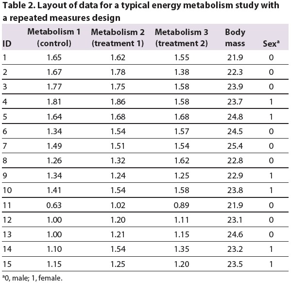
When you are using a study design in which repeated measurements are performed on the same individual under different conditions (i.e. a paired or repeated measures design), the data need to be organised as shown in Table 2. The example shows a study in which the same 15 animals were measured under a control and two treatment conditions.

Table 2.

Layout of data for a typical energy metabolism study with a repeated measures design

Formatting data for use with ‘R’

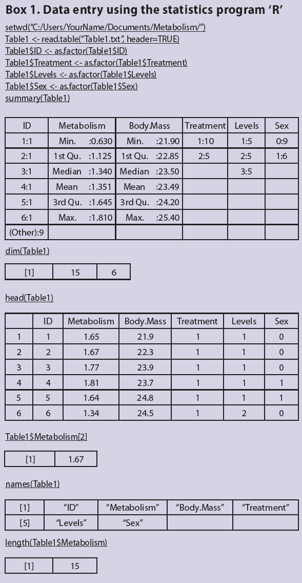
If using the statistics package R, note that it works in a slightly different way than MINITAB and SPSS. In R, functions are entered into a script editor and these functions are sent to the R terminal to be processed. Scripts can be written using the built-in script editors in R or via external script editors [e.g. Rstudio (www.rstudio.org) or Tinn-R (www.sciviews.org/Tinn-R/)]. Scripts can be saved and re-opened, thus allowing users to easily re-run and edit the analyses they want to perform. In this article, commands entered into the script editors are underlined and the output is shown in the tables within the box (note that not all commands result in an output).

Before importing data, the working directory must be specified using the setwd() function (this path will be user-specific). The working directory is the location where all data files are stored and where all outputs from R (e.g. figures) will be saved. Tab-delimited .txt files are imported into R using the read.table() function. Imported data are called data frames (e.g. Table1). Note that R is a case-sensitive language. Names are assigned to data frames and vectors using ‘<-’. Variables within a data frame are referred to using the following syntax: dataframe$variable (e.g. Table1$ID). Spaces are not allowed in data frame or variable names. Spaces within variable names in .txt files are replaced with periods when the .txt files are imported. For help on all functions, enter, e.g. ‘help(read.table)’.

Before proceeding, all categorical variables (e.g. ID, treatment, levels and sex) must be specified as factors using the as.factor() function. Ensure that you also do this after importing the data in Table 2. To ensure that the data has been imported correctly and all variables are specified correctly, the summary() function can be used. The dim() function can be used to ensure that the data frame is the correct size (i.e. Table 1 is 15 rows by 6 columns). The head() function can be used to see the first 6 rows of data. If you want to see the entire data frame, or a variable within a data frame, enter their names: e.g. Table1 or Table1$Metabolism. To refer to a specific value in a vector, for example the second value in the Table1$Metabolism, enter: Table1$Metabolism[2]. The names() function can be used to see all variable names within a data frame. To determine the number of elements in a variable, the length() function can be used (see Box 1 for an example).

The algorithm

Once the data have been entered into the statistics package of your choice using the above format, you are ready to use the algorithm. Beginning with step 1 below, work your way through the algorithm, deciding where to go next according to the results of the analyses at each step. In all steps, the statistical tests that should be used are indicated in bold capital letters. The analysis is finished when you get to step 39: the ‘END’ statement. A flowchart of the 39 steps of the algorithm (Fig. 1) allows you to see where you are in the overall analysis process at any stage.

Fig. 1.

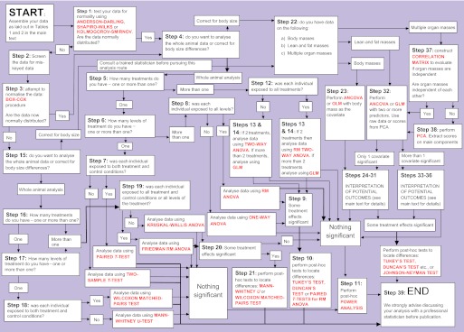
‘The 39 steps’: an algorithm for analysis of food intake and energy expenditure data. Statistical tests are shown in red text. For more details on each step in the flowchart, refer to the step-by-step instructions in the main text of this article. For instructions on applying this analysis using the statistics packages SSPS, MINITAB or R, see supplementary material Appendices I, II or III, respectively. GLM, general linear modelling; PCA, principal components analysis; RM ANOVA, repeated measures ANOVA.

Step 1. Are the data for the variables you are testing normally distributed? Use, for example, the ANDERSON-DARLING, SHAPIRO-WILKS or KOLMOGOROV-SMIRNOV test to determine the distributions. You need to do this for the dependent variable (food intake or energy expenditure) and the predictor variables (body mass or body composition). If the data are not normally distributed, go to step 2. If they are normally distributed, go to step 4.

Step 2. Check that the lack of normality in the data are not due to any mistyped data items etc. If it is due to typographical error, correct this error and go back to 1. If data are OK, go to step 3. NOTE: An easy way to check if there are typographical errors in a large data set is to plot the data as a histogram, or plot two columns of continuous data against each other. Any outlying data points will be immediately apparent, and you can then check whether they were mistyped.

Step 3. Attempt to normalise the distribution by transforming it. Applying the square root or log conversion will often normalise skewed data. More sophisticated transformations involve the BOX-COX procedure. After transformation, go back to step 1 to check if the data are normalised. If this normalises the distribution, go to step 4. If the distribution is still not normal, go to step 15.

Step 4. Do you want to analyse the whole animal data (go to step 5) or do you want to correct the data for differences in body size (go to step 22)?

Step 5. How many treatments (e.g. diet, drug, temperature) do you have? (Remember to distinguish separate treatments from levels of the same treatment; i.e. different doses of the same drug are levels, but different drugs are different treatments.) If you have just one treatment, go to step 6. If more than one treatment, go to step 12.

Step 6. How many levels are there? If there are just two levels (e.g. one treatment level and control) go to step 7. If there are more than two levels go to step 8.

Step 7. Was each individual exposed to both treatment levels? If no, analyse the data using TWO-SAMPLE T-TEST. If yes, analyse data using PAIRED T-TEST. Was the test result significant according to the accepted P-value of less than 0.05? If yes, go to step 39: END. If no, go to step 11. NOTE: you should not mix the design here. Either all of the individuals should appear just once (i.e. either in control or treatment groups), or all individuals should appear twice (i.e. in both treatment and control groups).

Step 8. Was each individual exposed to all the treatment levels? If no, analyse the data using ONE-WAY ANALYSIS OF VARIANCE (ANOVA) with treatment as a fixed factor. If yes, analyse the data using REPEATED MEASURES ONE-WAY ANOVA with treatment as the factor. (An alternative is to use ONE-WAY ANOVA with individual as a random factor.) Go to step 9.

Step 9. Was the treatment effect significant? If yes, go to step 10. If no, go to step 11.

Step 10. If the treatment was significant, you can probe exactly where the pair-wise differences are located in the data between treatment levels using a post-hoc comparison test. There are many to choose from, including TUKEY'S TEST or DUNCAN'S MULTIPLE RANGE TEST. For repeated measures, analyse using ANOVA probe difference using PAIRED T-TESTS. Go to step 39: END.

Step 11. Perform POWER ANALYSIS to evaluate power of the test. A power of 80% or greater is generally considered sufficient to make a strong statement about the absence of an effect. Lower levels of power mean the absence of an effect has a greater possibility of being a type 2 error. A power below 20% indicates that a statement that there is no effect is very dubious. Go to step 39: END.

Step 12. If you only have two treatments (e.g. diet and drug) or two factors (e.g. diet and sex), go to step 13. Otherwise go to step 14.

Step 13. If each individual did not receive all treatments, analyse the data using TWO-WAY ANOVA. If individuals received all treatments, use REPEATED MEASURES TWO-WAY ANOVA or GENERAL LINEAR MODEL with individual as a random factor. If you have significant effects (i.e. if the P-value for any effect is less than 0.05) go to step 10. If effects are not significant, go to step 11.

Step 14. If you have more than two treatments, you can analyse the data at this point using higher level ANOVAs (i.e. 3-WAY, 4-WAY etc.); another option is to use the GENERAL LINEAR MODEL. To start this part of the analysis, define each factor in the model and all of the higher-level interactions. Run the analysis. If higher-level interactions are not significant, remove them and re-run the model. Note that you cannot remove a non-significant primary treatment variable if it has a significant higher-level interaction. Successive removal of non-significant interactions yields the simplest significant model. Alternatively, different models can be evaluated using the AKAIKE INFORMATION CRITERION TEST (AIC TEST). If you have significant effects go to step 10. If effects are not significant, go to step 11.

Step 15. You have reached this step because it seems your data are not normally distributed. If you wish to analyse the whole animal data without correcting for body size differences, then a series of non-parametric statistical tests are available. However, if you want to correct for body size differences, then non-parametric tests are not readily available to do this. If the deviation from normal is not large, you can probably proceed with the parametric tests. We advise taking advice from a qualified statistician on whether your data are appropriate for these analyses. Do you want to analyse the whole animal data (go to step 16), or do you want to correct the data for body size differences (go to step 22)?

Step 16. How many treatments do you have (i.e. diet, drug, temperature etc.)? Remember to distinguish separate treatments from levels of the same treatment (i.e. different doses of the same drug are levels, but different drugs are different treatments). If just one treatment, go to step 17. If more than one treatment, go to step 19.

Step 17. How many levels are there? If just two levels (e.g. one treatment and control) go to step 18. If more than two levels, go to step 19.

Step 18. Was each individual exposed to both treatment levels? If not, analyse data using MANN-WHITNEY U-TEST. If yes, analyse data using WILCOXON MATCHED-PAIRS TEST. Was the test result significant according to the accepted P-value of less than 0.05? If yes, go to step 39: END. If no, go to step 11.

Step 19. Was each individual exposed to all of the treatments and levels? If not, analyse data using KRUSKAL-WALLIS ANOVA with treatment(s) as the factor(s). If yes, one option is to analyse the data using the REPEATED MEASURES FRIEDMAN TEST (ANOVA) with treatment(s) as the factor(s). Go to step 20.

Step 20. Was the treatment effect significant? If yes, go to step 21. If not, go to step 11.

Step 21. If the treatment was significant, you can probe exactly where the pairwise differences are located in the data between treatment levels using a post-hoc comparison test (MANN-WHITNEY U-TEST). For repeated measures, probe difference using WILCOXON MATCHED-PAIRS TEST. Go to step 39: END.

Step 22. Do you have:

1. measures of body size (e.g. length) or whole body mass? Go to step 23.

2. measures of lean and fat mass, e.g. from magnetic resonance spectroscopy (MRS) or dual-energy X-ray absorptiometry (DXA)? Go to step 32.

3. measures of multiple organ masses? Go to step 37.

Step 23. Analyse the data using ANALYSIS OF COVARIANCE (ANCOVA) or the GENERAL LINEAR MODEL. Enter the treatment variable as a dependent or response factor. If the same individuals were exposed to multiple treatment levels, or treatments, then include individual into the model as a random factor. Include the body size variable values as a covariate in the analysis. Include also the covariate by treatment-factor interaction. If the interaction is not significant, remove it and re-run the analysis. Go to step 24.

Step 24. If the treatment, covariate and interaction effects are all non-significant, go to step 11. Steps 25-31 detail how to interpret all of the other potential outcomes from the analysis detailed in step 23. Go to step 25.

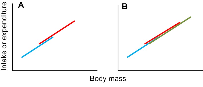
Step 25. If the covariate effect is significant, but there are no treatment or interaction effects (including a continued covariate effect and no treatment effect after the interaction has been removed), the results mean that a difference between the different treatment levels that was picked up in an analysis of whole body levels (i.e. in steps 1-21 above) is due only to the difference in size between the different treatment groups. In other words, there is no treatment effect on expenditure (or intake) above that caused by the effects of treatment on body mass (or size). That is, the plot of intake or expenditure against body mass looks like Fig. 2A (if there are two treatment levels) or Fig. 2B (if there are multiple treatment levels) (treatment levels are shown in red, green and blue). If this was not your result, go to step 26. Otherwise go to step 39: END.

Fig. 2.

Relationships between intake or expenditure and body mass when there is a significant mass effect but no significant treatment effect.

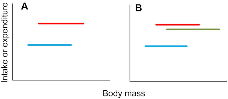
Step 26. If the treatment effect is significant, but there are no covariate or interaction effects (including a treatment effect and no covariate effect after the interaction has been removed – as occurred in step 24), this means that the effect of body mass on intake or expenditure is non-significant, but that there are significant differences between treatment levels. That is, the plot of intake or expenditure against body mass looks like Fig. 3A (if there are two treatment levels) or Fig. 3B (if there are multiple treatment levels) (treatment levels in red, green and blue). If you had multiple treatment levels (e.g. as illustrated in Fig. 3B) and this was your result, go to step 27. If this was not your result, go to step 28.

Fig. 3.

Relationships between intake or expenditure and body mass when there is a significant treatment effect but no significant mass effect.

Step 27. To find out which treatment levels differ from each other in the situation illustrated in Fig. 3B above, use a post-hoc multiple-comparison test such as the TUKEY'S TEST or DUNCAN'S MULTIPLE RANGE TEST. For example, in the case illustrated in Fig. 3B, it could be that the intake or expenditure of the blue group is significantly lower than the red and green groups, which do not differ from each other. Go to step 39: END.

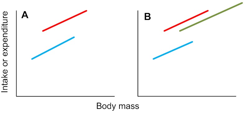
Step 28. If the treatment effect is significant and the covariate is significant, but the interaction is not significant (and the treatment and covariate effects remain when the interaction is removed), this means that there is an effect of body weight on intake or expenditure; on top of this, there is also a treatment effect. That is, the plot of intake or expenditure against body mass looks like Fig. 4A (if there are two treatment levels) or Fig. 4B (if there are multiple treatment levels) (treatment levels are shown in red, green and blue). If you had multiple treatment levels and your result was as shown in Fig. 4B, go to step 29. If this was not your result, go to step 30.

Fig. 4.

Relationships between intake or expenditure and body mass when there is a significant treatment effect and a significant mass effect.

Step 29. The key point about the result described in step 28 is that there is no significant interaction effect. This means that the lines in the plots shown in Fig. 4 all run parallel to each other. The difference between the treatment levels is the same at all body sizes. To find out which treatment levels differ from each other in the situation illustrated in Fig. 4B above, use a post-hoc multiple-comparison test such as the TUKEY'S TEST or DUNCAN'S MULTIPLE RANGE TEST. In this case, the test needs to be performed taking the body mass effect into account. Most statistical packages include this comparison option among the output options for the general linear model or ANCOVA. Go to step 39: END.

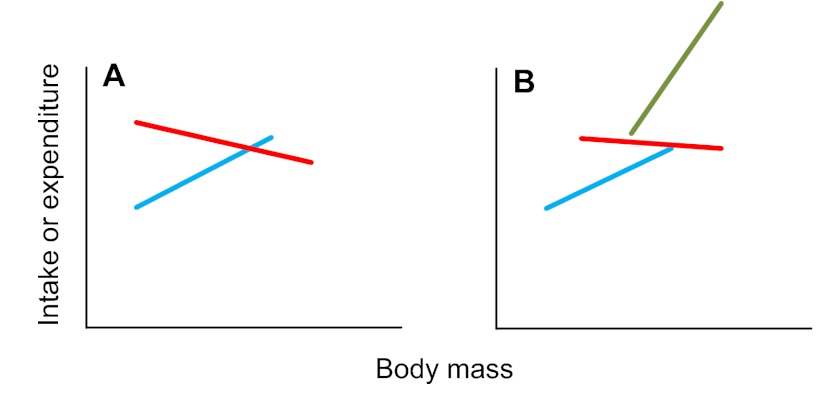
Step 30. If the treatment effect is significant and the covariate is significant, but the interaction is also significant, this means that there is an effect of body mass on intake or expenditure. On top of this, there is also a treatment effect, but that treatment effect differs depending on the treatment level. That is, the plot of intake or expenditure against body mass looks like Fig. 5A (if there are two treatment levels) or Fig. 5B (if there are multiple treatment levels) (treatment levels are shown in red, green and blue). If you had multiple treatment levels and your result was as shown in Fig. 5B, go to step 31. If this was not your result go to step 39: END.

Fig. 5.

Relationships between intake or expenditure and body mass when there is a significant treatment effect and a significant mass effect and a significant interaction effect.

Step 31. The key point about the plots in Fig. 5 is that the lines do not run parallel. This means that, at some point, the lines must cross. The issue of testing for the treatment level effects, therefore, boils down to determining the range of values on the x-axis between which the lines are significantly separated. This test is called the JOHNSON-NEYMAN TEST. This test only works for situations like that shown in Fig. 5A, where there are two levels. To address the situation shown in Fig. 5B, there is no single overall test; the different levels need to be compared separately on a pair-wise basis. Go to step 39: END.

For instructions on performing the JOHNSON-NEYMAN TEST, see White (White, 2003). This test is not available as an option in SPSS, MINITAB or R, and needs to be calculated manually.

Step 32. If you have measures of lean and fat mass available (for example, from MRS or DXA analyses), or data from a principal components analysis (PCA) derived in step 38, analyse the data using ANCOVA or the GENERAL LINEAR MODEL (for detailed instructions see step 9 above). Enter the treatment variable as a fixed factor. If the same individuals are exposed to multiple treatment levels, or treatments, then include individual into the model as a random factor. Include the fat mass and lean mass as independent covariates in the analysis. The assumption of the test is that the fat mass and lean mass are independent. This is often not true and should be borne in mind when interpreting the data. Include also all the covariate-by-treatment factor interactions. Once the analysis has been run, check whether higher-level interactions are non-significant; remove them from the model and then re-run the analysis until the model is maximally simplified. Because there are two covariates in this analysis, the outcomes are potentially more complex. The extra covariate effect can be envisaged as a third dimension in the output plots. If one of the covariates is non-significant, the interpretations resolve down to those with a single covariate (go to step 24 and progress from there). If both of the covariates are significant, the interpretations are as follows – go to step 33. If the treatment and both covariates are non-significant, go to step 11.

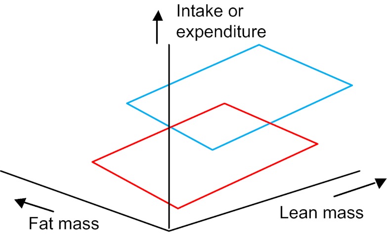
Step 33. Both of the covariates are significant, the treatment effect is significant but there are no significant interactions. This situation can be envisaged as two planes that are overlaid in parallel with each other (Fig. 6).

Fig. 6.

3D plot showing intake or expenditure (vertical axis) in relation to both fat and lean body mass in a situation where there are significant mass effects and a significant treatment effect but no interactions.

The key thing to note about Fig. 6 is that the planes lie a fixed distance apart. This is the treatment effect. If there are only two treatment levels and the treatment effect is significant, then you can infer that the difference between the planes at all fat and lean masses is significant. If there are multiple levels, then the next step is to analyse which planes differ from each other using a post-hoc multiple-comparison test (e.g. TUKEY'S TEST or DUNCAN'S MULTIPLE RANGE TEST). Note that these tests need to be done as an option within the GLM, rather than as separate tests. In this way, the covariate effects are accounted for. If this was not your result, go to step 34. Otherwise go to step 39: END.

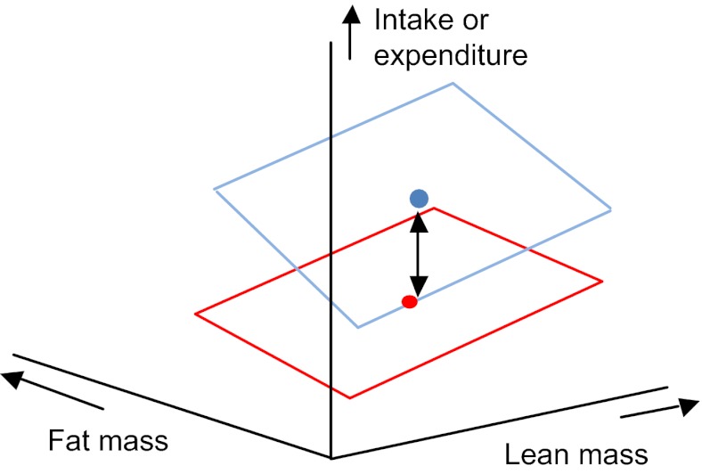
Step 34. The treatment effect is significant, both covariates are significant, one of the covariate-by-treatment interactions is also significant, but there is no covariate-by-covariate interaction. This result represents an effect that can be illustrated as shown in Fig. 7. If the fat-by-treatment effect is significant, this means that the gradient of the mass effect is different for the two treatment levels, but that the planes are parallel along the lean mass axis because there is no lean-by-treatment interaction.

Fig. 7.

3D plot showing intake or expenditure (vertical axis) in relation to both fat and lean body mass in a situation where there are significant mass effects and a significant treatment effect and a significant fat mass by treatment interaction but no lean mass by treatment interaction or covariate by covariate interaction.

In this situation, the first step is to normalise the data for both fat and lean mass, and then compare treatments using a post-hoc multiple-comparison test (e.g. TUKEY'S TEST or DUNCAN'S MULTIPLE RANGE TEST). This effectively only asks if the treatment is significant at the average lean and fat mass – i.e. at the central point of each plane indicated by blue and red dots in Fig. 7. A more sophisticated analysis would be proceed in two stages: (1) normalise the data for fat mass and perform the same test and (2) go back to the original data and normalise for lean mass, and then perform the JOHNSON-NEYMAN TEST to ask at what fat masses the effect of treatment is significant. If both covariate-by-treatment interactions are significant, go to step 35. Otherwise go to step 39: END.

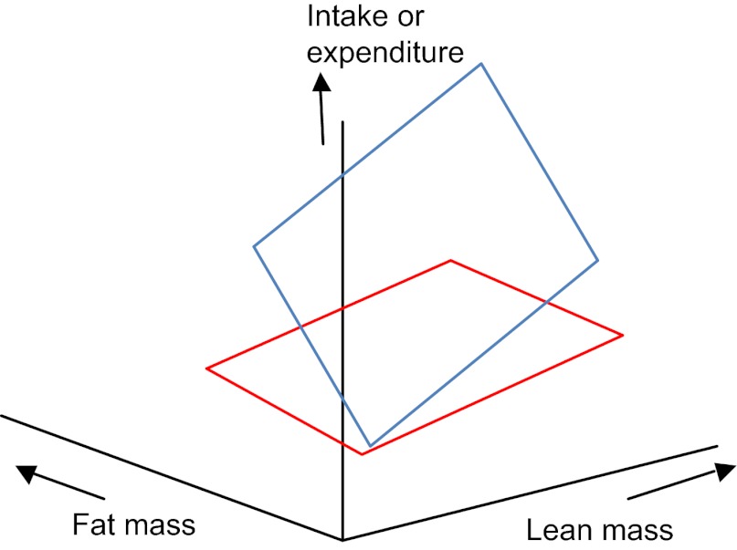
Step 35. When both the covariates and treatment are significant, and both of the treatment-by-covariate interactions are significant, but there is no covariate-by-covariate interaction, the effect can be illustrated by the plot shown in Fig. 8. In this situation, the upper plane is not parallel to the lower plane in either lean or fat dimensions. In this situation, one can normalise the data for both fat and lean mass, and then compare treatments using a post-hoc multiple-comparison test (e.g. TUKEY'S TEST or DUNCAN'S MULTIPLE RANGE TEST).

Fig. 8.

3D plot showing intake or expenditure (vertical axis) in relation to both fat and lean body mass in a situation where there are significant mass and treatment effects and both a significant fat mass by treatment interaction and a significant lean mass by treatment interaction but no covariate by covariate interaction.

Again, this effectively only asks if the treatment is significant at the average lean and fat mass – i.e. at the central point of each plane. A more sophisticated analysis would be to again proceed in two stages: (1) normalise the data for fat mass, and then perform the JOHNSON-NEYMAN TEST to ask at what lean masses the effect of treatment is significant and (2) go back to the original data and normalise for lean mass and then perform the JOHNSON-NEYMAN TEST to ask at what fat masses the effect of treatment is significant. If the covariate-by-covariate interaction is also significant, this is the most complex situation of all: go to step 36. Otherwise, go to step 39: END.

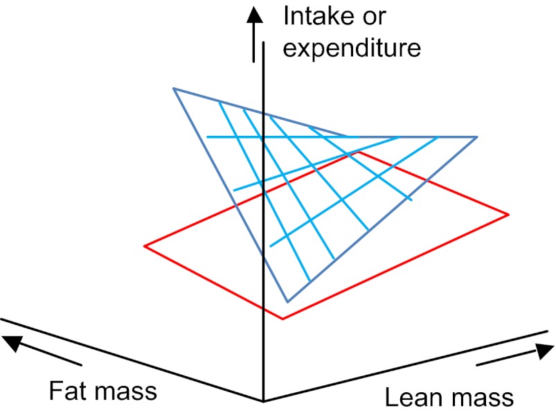
Step 36. When the covariate-by-covariate interaction is significant, the planes no longer remain flat. This is illustrated in Fig. 9. In this instance, there is a strong positive effect of the treatment on fat mass when lean mass is low, but a strong negative effect when lean mass is high. In this situation, unless the sample size of individuals is very high, the best way to proceed is to plot the actual data in a 3D plot, and to overlay theoretical planes from the derived model parameters to illustrate how the planes interact. Go to step 39: END.

Fig. 9.

3D plot showing intake or expenditure (vertical axis) in relation to both fat and lean body mass in a situation where there are significant mass and treatment effects as well as significant mass by treatment and covariate by covariate interactions.

Step 37. If you have multiple organ masses, then each organ mass can be entered as a covariate in the GENERAL LINEAR MODEL analysis described above for the situation where lean and fat mass are known. This then becomes a multidimensional extension of the situations illustrated in 32-36. Such an analysis is not possible to represent graphically. It is important to recognise that the use of multiple predictors assumes that the predictors are independent of each other. The first step in this analysis is therefore to construct a CORRELATION MATRIX showing the correlation coefficients between all of the pair-wise organ masses. If the correlation matrix indicates that the organ masses are largely independent of each other, go to step 32 and enter the individual organs as independent predictors in the GLM. If the correlation matrix indicates that there are significant correlations between the organ masses across individuals, go to step 38.

Step 38. An alternative approach if there are high numbers of correlated predictor variables is to re-describe the variation using a PRINCIPAL COMPONENTS ANALYSIS. This generates scores for each individual along a number of uncorrelated predictor variables from the original data matrix that can then be used as predictors in the GENERAL LINEAR MODEL (see e.g. Selman et al., 2005). The advantage of using this approach is that the uncorrelated predictor variables are statistically independent and hence this is a more valid statistical procedure. Unfortunately, the principal components are sometimes difficult to interpret biologically. You must therefore either proceed with the raw data, as in step 37 (which is statistically suspect but generally biologically easier to interpret) or carry out the procedure in this step (which is statistically appropriate but difficult to interpret biologically). Once you have generated scores on the principal component axis, go to step 32 and enter these scores as independent predictors in the GLM analysis.

Step 39. Remember to consult with a trained statistician before publishing results generated by this algorithm. END.

Suggestions for publication of statistics

Following Tschöp et al. (Tschöp et al., 2012), we recommend that the use of histograms to compare treatment groups should be avoided whenever possible, when preparing publications. Instead, we recommend that the dependent variable is plotted against either body mass or lean body mass.

Alongside this type of plot, the results of the ANCOVA should be presented; these should include the F-values, degrees of freedom and P-values for the treatment effect, each covariate (e.g. fat mass and lean body mass), and the interactions.

Where it is claimed that there is no significant effect of a given treatment, the results of a power analysis should be included, stating the power of the particular analysis to detect a given effect size. For example, “This analysis had a power of 40% to detect an effect size of 10% between the treatment and control groups”.

Conclusion

Analysis of energy-intake and expenditure data is complex and involves several key issues: notably, the problems of having sufficient power to establish a treatment effect and how to overcome the pervasive impact of individual differences in body mass. We hope this step-by-step guide and the attached flowchart will assist readers in carrying out the most appropriate statistical approaches for these issues, and thereby avoid the common pitfalls of such analysis.

References

- Allison D. B., Paultre F., Goran M. I., Poehlman E. T., Heymsfield S. B. (1995). Statistical considerations regarding the use of ratios to adjust data. Int. J. Obes. Relat. Metab. Disord. 19, 644-652 [PubMed] [Google Scholar]
- Arch J. R., Hislop D., Wang S. J., Speakman J. R. (2006). Some mathematical and technical issues in the measurement and interpretation of open-circuit indirect calorimetry in small animals. Int. J. Obes. (Lond.) 30, 1322-1331 [DOI] [PubMed] [Google Scholar]
- Butler A. A., Kozak L. P. (2010). A recurring problem with the analysis of energy expenditure in genetic models expressing lean and obese phenotypes. Diabetes 59, 323-329 [DOI] [PMC free article] [PubMed] [Google Scholar]
- Kaiyala K. J., Schwartz M. W. (2011). Toward a more complete (and less controversial) understanding of energy expenditure and its role in obesity pathogenesis. Diabetes 60, 17-23 [DOI] [PMC free article] [PubMed] [Google Scholar]
- Kleiber M. (1932). Body size and metabolism. Hilgardia 6, 315-353 [Google Scholar]
- Kleiber M. (1961). The Fire of Life: An Introduction to Animal Energetics. New York, NY: Wiley [Google Scholar]
- Lighton J. R. B. (2008). Measuring Metabolic Rates, a Manual for Scientists. Oxford: Oxford University Press [Google Scholar]
- Poehlman E. T., Toth M. J. (1995). Mathematical ratios lead to spurious conclusions regarding age- and sex-related differences in resting metabolic rate. Am. J. Clin. Nutr. 61, 482-485 [DOI] [PubMed] [Google Scholar]
- Rubner M. (1883). Über den einfluss der körpergrösse auf stoff- und kraftwechsel. Z. Biol. 19, 536-562 [Google Scholar]
- Selman C., Phillips T., Staib J. L., Duncan J. S., Leeuwenburgh C., Speakman J. R. (2005). Energy expenditure of calorically restricted rats is higher than predicted from their altered body composition. Mech. Ageing Dev. 126, 783-793 [DOI] [PubMed] [Google Scholar]
- Sokal R. R., Rohlf F. J. (2012). Biometry: The Principles and Practice of Statistics in Biological Research, 4th edn. New York, NY: Freeman [Google Scholar]
- Speakman J. R. (2010). FTO effect on energy demand versus food intake. Nature 464, E1, discussion E2. [DOI] [PubMed] [Google Scholar]
- Tschöp M. H., Speakman J. R., Arch J. R., Auwerx J., Brüning J. C., Chan L., Eckel R. H., Farese R. V., Jr, Galgani J. E., Hambly C., et al. (2012). A guide to analysis of mouse energy metabolism. Nat. Methods 9, 57-63 [DOI] [PMC free article] [PubMed] [Google Scholar]
- White C. R. (2003). Allometric analysis beyond heterogeneous regression slopes: use of the Johnson-Neyman technique in comparative biology. Physiol. Biochem. Zool. 76, 135-140 [DOI] [PubMed] [Google Scholar]
- Zar J. H. (2009)Biostatistical Analysis, 5th edn. New York, NY: Wiley [Google Scholar]
Associated Data
This section collects any data citations, data availability statements, or supplementary materials included in this article.