Evaluation of Sparse-view Reconstruction from Flat-panel-detector Cone-beam CT

Abstract

Flat-panel-detector X-ray cone-beam computed tomography (CBCT) is used in a rapidly increasing host of imaging applications, including image-guided surgery and radiotherapy. The purpose of the work is to investigate and evaluate image reconstruction from data collected at projection views significantly fewer than what is used in current CBCT imaging. Specifically, we carried out imaging experiments by use of a bench-top CBCT system that was designed to mimic imaging conditions in image-guided surgery and radiotherapy; we applied an image reconstruction algorithm based on constrained total-variation (TV)-minimization to data acquired with sparsely sampled view-angles; and we conducted extensive evaluation of algorithm performance. Results of the evaluation studies demonstrate that, depending upon scanning conditions and imaging tasks, algorithms based on constrained TV-minimization can reconstruct images of potential utility from a small fraction of the data used in typical, current CBCT applications. A practical implication of the study is that the optimization of algorithm design and implementation can be exploited for considerably reducing imaging effort and radiation dose in CBCT.

I. Introduction

Flat-panel-detector X-ray cone-beam computed tomography (CBCT) is used in a rapidly increasing host of imaging applications. Although current flat-panel-detector CBCT (for convenience, we simply refer to flat-panel-detector CBCT as CBCT throughout the paper) is not designed generally for achieving image quality of advanced diagnostic CT in terms of spatial, contrast, and temporal resolution, it can yield images containing information of high practical utility in image-guided interventions and have a greater scanning-configuration flexibility than diagnostic CT. C-arm CBCT in surgery and on-board CBCT in radiotherapy represent two examples of medical CBCT applications for determining the position and status of a target area and the surrounding tissues inside a patient.

As in diagnostic CT, radiation dose to the subject in CBCT imaging is also a paramount concern. In particular, when CBCT is used for guiding and evaluating interventional procedures, repeated scans of the same subject are carried out, such as multiple scans during a surgical operation or over the course of fractionated radiation therapy. Therefore, the accumulated radiation dose of repeated CBCT imaging to the patient poses a serious radiation safety concern. Studies indicate that dose from CT scans may have a lifetime attributable risk of cancer higher than previously assumed [1]–[3], Reducing CT dose has been an area of active research in medical imaging. In CBCT, one can reduce imaging dose by reducing the number of projection views at which data are collected. The use of fewer projection views can also lead to a reduced imaging time in step-and-shoot CBCT, improving workflow, and minimizing potential motion artifacts. However, reducing the number of projection views leads to a challenging image-reconstruction task. When the projection views are sparsely sampled, the analytic reconstruction algorithms [4]–[7], which require densely sampled projection views, can result in prominent streak artifacts [8], [9]. Efforts have been made to interpolate additional projection views from measured data [10], [11]. Such an approach may be useful for certain scanning configurations and particular subjects. It is, however, difficult to make general conclusions about the practical utility of such an approach. Prior efforts exist in developing algorithms for image reconstruction from parallel-and fan-beam projections [12], [13] or cone-beam projections of sparse objects [14] acquired at a small number of views, some of which can be extended to image reconstruction from CBCT data acquired at a reduced number of views.

Initial articles [15], [16], which led off the study of compressive sensing (CS) as a distinct field, showed examples of image reconstruction from ideal, sparse Fourier data by use of constrained minimization of the image’s total variation (TV). The illustrated Fourier sampling patterns, and results, were highly suggestive and encouraging for sparse-view sampling in CT. Recent work on translating constrained TV-minimization to application with divergent-beam transforms indeed showed, largely in simulation, that highly accurate image reconstruction from sparsely sampled projection views may be possible [17]. An adaptive steepest descent-projection onto convex sets (ASD-POCS) algorithm, for accurately solving constrained TV-minimization with the divergent-beam transform was formalized [17], [18]; the ASD-POCS algorithm combines steepest descent on the image TV with an adaptive step size and POCS to enforce image constraints, including a tolerance on the data divergence.

Under ideal conditions of noiseless simulation, it appears that sparse-view sampling in CT can yield exact reconstruction. But theoretically there is, as yet, no proof of an exact recovery principle (ERP) [15] for the divergent-beam transform. Our limited study on the 2D Radon transform [19] using the restricted isometry principle (RIP) [20] yields very large isometry constants, which would seem to exclude an ERP. Yet, these sampling configurations appear to yield highly accurate reconstruction in simulation even with challenging phantoms designed to “break” the algorithm. This apparent contradiction, however, is likely due to the fact that CS theory for deterministic sampling is not yet mature enough to be applied to the X-ray transform. A goal of the present work is to carry out a comprehensive study of the use of constrained TV-minimization for sparse-view reconstruction of real CT data, which contain various non-idealities with respect to the ideal imaging model. In the study, data were collected in two imaging experiments using a bench-top CBCT system that was designed to mimic imaging conditions in image-guided surgery and radiotherapy. We show that the ASD-POCS algorithm for solving constrained TV-minimization is effective at mitigating artifacts that often dominate sparse-view image reconstruction.

A major question, hardly addressed in the literature, is that, even though algorithms based on constrained TV-minimization appear to effectively remove streaks, other aspects of image quality have never been carefully analyzed. Indeed, application of TV regularization is criticized often for producing blocky, cartoonish images. To address this concern, we display a multitude of images showing various ROIs at different contrast levels. In addition to this, we employ a spectrum of quantitative performance metrics from the image science literature with the purpose of rigorously elucidating image quality characteristics of resulting reconstructions, including image noise, correlation, similarity (to a “true” reference image,) and task-based detectability. In particular, some metrics can be impacted by subjective qualities such as blockiness. To gauge the performance of the ASD-POCS algorithm, we also included reconstruction and evaluation results obtained with carefully coded implementations of the expectation-maximization (EM) [21], [22] and projection-onto-convex-sets (POCS) [23]–[25] algorithms.

We organize the paper as follows. In Sec. II, we discuss the bench-top CBCT system, data acquisition, and imaged subjects. In Sec. III, reconstruction algorithms, including the EM, POCS, and ASD-POCS algorithms, are described. A leading focus of the work is to carry out an extensive, quantitative evaluation of image quality. Therefore, we introduce in Sec. IV a number of evaluation metrics that are designed for characterizing different aspects of multi-faceted image quality. In Secs. V, VI, and VII, we present and analyze in detail the study results, which are followed by discussion and conclusion in Sec. VIII and IX.

II. CBCT system and data acquisition

A. CBCT system

A bench-top CBCT system [26], developed to simulate imaging tasks in image-guided surgery and radiotherapy, was used in this study. The X-ray tube has a 0.4–0.8 mm focal spot and 14° anode (Rad94 in Sapphire, Varian Medical Systems, Salt Lake City, UT,) powered by a constant potential generator CPX-380 (EMD Inc., Montreal, QC); the flat-panel detector, with a pitch of 400 μm, was based on a 1024×1024 (41×41 cm²) active matrix of a-Si:H photo diodes, thin-film transistors, and CsI:Tl X-ray converter (RID-1640A, PerkinElmer Optoelectronics, Santa Clara, CA); and the imaged subject was placed on a rotation stage. The distances of the source to the center of rotation and to the detector plane were 93.5 cm and 144.4 cm, respectively, yielding a field of view (FOV) of 26×26×26 cm³. In our experiments, to mimic typical imaging conditions in image-guided surgery and radiotherapy, we used a circular trajectory to collect data at 120 kVp exposure. In the imaging coordinate system, the trajectory is within a plane at z = 0 cm. We also added a filtration of 2.0 mm Al + 1.1 mm Cu to the source so that it yields beam quality comparable to that of clinical CT scanners. An anti-scatter grid was not used in the current study. The mAs per projection was 1.2 mAs. The dose (to the center of a 16cm water cylinder) therefore varied linearly from 0.39 mGy at 30 views to 12.43 mGy at 960 views, resulting an effective dose of about 0.023 mSv and 0.74 mSv to the head for 30 and 960 views.

B. Experimental phantoms

We used two phantoms: a cylindrical phantom and an anthropomorphic head phantom. Images displayed in row 1 of Fig. 1 were reconstructed from full, 960-view data by use of the FDK algorithm. Because the “truth” of the physical phantoms is unknown, we use the images as the surrogate “truth” and refer to them as the FDK-reference images.. The cylindrical phantom is formed of 16 cm diameter SolidWater^™ material (Gammex RMI, Madison WI), containing six different tissue-simulating plastic inserts with electron densities approximating cortical bone (2x), breast, brain, liver, and adipose tissue. In addition, the central region of the cylindrical phantom also has an air pencil-chamber cavity with an inserted thin wire. Although the spatial structure of the cylindrical phantom is relatively simple, different contrast levels offered by different inserts provide an opportunity to evaluate reconstruction contrast and spatial resolution. The anthropomorphic head phantom was designed for realistically simulating human head [27], it features not only a natural human skeleton but also contrast-detail spheres approximating soft tissues. These fine and low-contrast structures pose challenges for tasks of image reconstruction from reduced numbers of projections and provide opportunities for evaluating algorithm performance.

Figure 1.

Images of the cylindrical and head phantoms within a transverse slice at z = 0 cm reconstructed from full data by use of the FDK (row 1) and ASD-POCS (row 2) algorithms. For the cylindrical-phantom, the entire images are displayed with a wide (i.e., bone-grayscale) window [−1000, 714] HU; rectangle regions enclosed by dashed lines (i.e., ROIs 1 and 2) are redisplayed in the upper-left and lower-left corners with a narrow (i.e., soft-tissue-grayscale) window [−257, 143] HU; and the rectangle region enclosed by solid lines (i.e., ROI 3) is re-displayed in the lower-right corner with a zoomed-in view in a grayscale window of [−1000, −143] HU, with an arrow pointing to a wire insert. For the head phantom, the entire images are displayed with a wide bone-grayscale window [−1000, 1000] HU; ROIs 1 and 2 are re-displayed in the upper-left and lower-left corners with a narrow window [−429, 429] HU; ROI 3 is re-displayed in the lower-right corner by use of a zoomed-in view with the bone-grayscale window.

C. Data acquisition

In the experiment, data were collected from each of the two phantoms with the detector at a rate of about 1 frame/second. We estimated reference measurements (i.e., I₀) by averaging the detector-pixel values over a selected region on the detector plane corresponding to the unattenuated beam. Subsequently, projection data were calculated from the reference and transmission measurements. In each of the two imaging experiments, we collected measurements at 960 views uniformly distributed over 2π and converted them into projection data. Throughout the paper, we refer to the 960-view data as the full data. Images displayed in Fig. 1 were reconstructed from the full data sets of the phantoms by use of the FDK and ASD-POCS algorithms, which, as mentioned above, were used as the surrogate truth for the corresponding phantoms and are referred to as FDK-reference and ASD-POCS-reference images. In the study below, we extracted sparse-view data from the full data.

III. Reconstruction Algorithms

A. Imaging model

In practical imaging applications, data g acquired, and image f reconstructed, can be interpreted as vectors of sizes M and N, i.e., g = (g₁, g₂, …, g_M)^T and f = (f₁, f₂, …, f_N)^T, where T denotes the matrix transpose, and M and N the numbers of transmission rays and image voxels. We assume that the imaging model in CBCT is a discrete linear system

$$\mathbf{g}=\mathcal{H}\mathbf{f},$$ (1)

where is an M × N system matrix modeling the cone-beam X-ray transform. With this discrete data model, image reconstruction can be thought of as an inversion of Eq. (1) given knowledge of the projection data. In practical CBCT imaging, the huge size of the linear system prevents one from directly inverting Eq. (1). Moreover, for problems such as image reconstruction from a reduced number of projections, the linear system can be severely under-determined, i.e., M ≪ N, admitting multiple solutions. Obviously, a particular entry of M depends on the selection of image-expansion basis set and the discrete computation of the X-ray transform. Throughout the work, we have used voxels as the image-expansion-basis set and a ray-driven projector for computing the X-ray transform.

B. EM and POCS algorithms for unconstrained optimization reconstruction

Optimization-based approach can be designed for reconstructing images, which generally consists of an optimization formulation and algorithms solving for the formulation. For the CBCT-imaging model in Eq. (1), an unconstrained minimization problem can be devised in which the objective function is the Kullback-Leibler (KL) divergence between the measured and estimated data [28]. It is well-known that the EM algorithm yields a solution to the unconstrained minimization problem through minimizing the KL-data divergence. In the work, for comparison, we implemented the EM algorithm and compared its reconstruction with those of other algorithms. Because POCS algorithm is used widely for solving a discrete linear system in Eq. (1) and because, as shown below, it is used as a component of the ASD-POCS algorithm, we also implemented the POCS algorithm and compared its reconstruction with those of other algorithms under study. In fact, when data are consistent with the imaging model in Eq. (1), the POCS algorithm solves an unconstrained minimization problem in which the object function is the Euclidean-data divergence

$$D(\mathbf{f})=\mid \mathcal{H}\mathbf{f}-\mathbf{g}\mid .$$ (2)

In the numerical studies described below, the POCS and EM algorithms were terminated at 240 and 300 iterations, which were chosen at which the Euclidean- and KL-data divergences change little for the cases under study. Throughout the study, f = 0 and 1 were used as the initial image estimates for POCS and EM algorithms, respectively.

C. ASD-POCS algorithm for constrained TV-minimization reconstruction

The POCS and EM algorithms provide solutions to unconstrained optimization problems in which the Euclidean- and KL-data divergences, respectively, are the objective functions. For under-sampled data, where M ≪ N the solution arrived at by these algorithms can generally be dependent on initial images. As discussed in detail previously [17], [18], [29], image reconstruction based upon Eq. (1) can also be formulated as a constrained optimization problem:

$${\mathbf{f}}^{\ast }=argmin{\left|\right|\mathbf{f}\left|\right|}_{\text{TV}}\text{s}.\text{t}.D(\mathbf{f})\le \epsilon \text{and}{f}_n\ge 0,$$ (3)

where ||f||_TV, referred to as the image TV, denotes the ℓ₁ norm of the discrete gradient magnitude of the image. This optimization formulation selects the image with minimum TV amongst those that satisfy the constraints, and the solution can be unique even when M ≪ N. The data divergence D can reach zero in the absence of data inconsistency. In practice, however, measurements always contain inconsistent components, and a tolerance parameter ε (discussed further below) is selected for controlling the impact level of potential data inconsistency on image reconstruction [18].

We point out here that there is a distinction between an iterative reconstruction algorithm and the optimization formulation upon which an algorithm is based. For example, the iteration of the EM algorithm is often truncated well short of convergence to the minimizer of the KL-data divergence. One of the themes of this work is to investigate the properties of the solution to Eq. (3). To attain this, we employed the same ASD-POCS algorithm as that described in detail in Ref. [18] to accurately solve the constrained TV-minimization problem in Eq. (3). An efficient form of ASD-POCS was developed for application to digital breast tomosynthesis [30]. But the algorithm was designed to yield clinically useful images in less than 20 iterations, and not necessarily to solve constrained TV-minimization. As there is no proof of convergence for ASD-POCS, we have derived necessary conditions for convergence [18]. First, The image constraints must be satisfied: f ≥ 0 and D(f) ≤ ε. The latter constraint is satisfied with equality, because the zero-TV image lies outside the data tolerance constraint if there is something in the CBCT scanner. Second, there is a parameter c_α, which can be computed from an image estimate [18]. Physically, this parameter is the cosine of an angle in the N-dimensional space of images; this angle lies between the gradient vectors of the data divergence and image TV; and these vectors should be back-to-back or, equivalently, c_α should be −1, at the solution to Eq. (3). Due to the high dimensionality of the space of images, c_α is a quite sensitive parameter, and it has been our experience that, with actual scanner data, changes to the image estimate become imperceptible when c_α < −0.5 and the image constraints are satisfied.

In the present study, a modification was made to the ASD-POCS algorithm for improving its convergence in solving the constrained optimization problem in Eq. (3). This modification involves employing the POCS-step to reduce the data divergence until about 80 iterations, after which gradient descent is employed for reducing the data-divergence. With this modification, accurate solutions to Eq. (3) are obtained within 200 iterations. We point out that this ASD-POCS algorithm is developed in the spirit of a plug-and-play algorithm, as discussed in Ref. [29], and contains adaptive steps that make proof of convergence quite difficult, if not impossible. On the other hand, resulting images are checked against the necessary optimality conditions, c_α = −1, f ≥ 0, and D(f) = ε.

The motivation for solving Eq. (3) accurately is two-fold: (1) for a given system matrix and data set g, the reconstructed image is only a function of ε; and (2) assuming that an ERP exists for CBCT, the solution to Eq. (3) may be highly accurate for small ε. Small ε constrains the possible images so that the estimated data agrees closely with the available data. In general, ε must be larger than 0 in order for there to be a feasible image because of inconsistency between the actual data and the system model. Relaxing ε (going to larger values) includes images with lower TV, thereby allowing for greater TV regularization. The spirit of CS-style image reconstruction involves solving Eq. (3) for small ε, which is technically challenging. Note that, with ideal data, CS calls for solving Eq. (3) with ε = 0. The idea is that the sparse-view sampling has a large null space, where many images could agree with the available data within a small ε. If an ERP exists for the system matrix, one can expect that the minimum-TV image with a tight ε could accurately represent the underlying object function. Indeed, it is likely that many over-regularized, blocky images, which arise from TV regularization, correspond to solving Eq. (3) with too large an ε. The POCS-data divergence provides a lower bound of ε, and we select a final ε in the neighborhood of the bound.

IV. Performance evaluation of image reconstruction

The performance of various TV-minimization-based algorithms in CT-image reconstruction has been evaluated in simulation studies [17], [18], [31], [32]. A focus of the work reported here is on evaluation of the ASD-POCS algorithm with real CBCT data in imaging experiments of potential practical significance. We also implemented the POCS and EM algorithms in order to establish a relative performance benchmark for the ASD-POCS algorithm. It should be pointed out that additional, different algorithms may be devised for solving the optimization problems mentioned in Secs. III-B and III-C and that additional, different optimization formulations and the associated algorithms may be devised for image reconstruction based upon the imaging model in Eq. (1). It is possible that these algorithms may yield potentially improved reconstruction. However, research on these optimization formulations and algorithms is beyond the scope of the current work.

A. Qualitative-visualization-based evaluation

In this study, we first conducted a qualitative evaluation by using visual inspection and comparison of reconstructed images. To reveal the structure and contrast details in a reconstruction, we also display selected regions of interest (ROIs) with a narrowed display grayscale and/or zoomed-in view, Although visual inspection of images provides only a qualitative comparison of algorithm performance, it can be an informative assessment of the image quality especially in the presence of image artifacts that are otherwise difficult to quantify meaningfully by use of general metrics. Images were displayed with separate grayscale windows to facilitate bone or soft-tissue visualization. When a narrow grayscale window is used, it may reveal considerable reconstruction artifacts that may be otherwise invisible in a wide grayscale window. In our study, we have used grayscale windows that are consistent between images reconstructed by use of different algorithms for purpose of comparison.

B. Quantitative-metric-based evaluation

It is well recognized that image quality is multiple faceted, depending upon the tasks for which images are reconstructed. This is particularly true in real-data studies in which the “truth” about the underlying object function is unknown. To evaluate different aspects of image quality in real-data studies under consideration, we also use a number of technical-efficacy-based metrics, which are illustrated below.

1) Image-similarity metrics

Currently, in a practical application of CBCT, an image, f₀ = (f₀₁, f₀₂, …, f_0N)^T, is reconstructed from full data by use of the FDK algorithm with a Hann filter, which is used as a surrogate truth. We first evaluate quantitatively the reconstruction quality by considering the following two metrics: universal quality index (UQI) [33] and mutual information (MI) [34], which can be used for measuring the degree of similarity between the reconstructed and FDK-reference images. It should be pointed out that the FDK-reference image f₀ is not the real “truth”, and as discussed in Sec. VII below, the use of different reference images in the computation of image-similarity metrics can lead to quantitatively different evaluation results. We use f₁ = (f₁₁, f₁₂, …, f_1N)^T to denote an image reconstructed from sparse-view data.

For a selected ROI within the reconstructed and reference images, we define image means, variances, and covariances over an ROI as

$${\overline{\text{f}}}_j=\frac{1}{N^{\prime }}\sum _{n=1}^{N^{\prime }}{f}_{jn},{\sigma }_j^2=\frac{1}{N^{\prime }-1}\sum _{n=1}^{N^{\prime }}{(f_{jn}-{\overline{\text{f}}}_j)}^2,$$ (4)

where j = 0 and 1, and

$$\text{Cov}\{{\mathbf{f}}_1,{\mathbf{f}}_0\}=\frac{1}{N^{\prime }-1}\sum _{n=1}^{N^{\prime }}(f_{1n}-{\overline{\text{f}}}_1)(f_{0n}-{\overline{\text{f}}}_0),$$ (5)

where N′ denotes the number of voxels within the ROI.

Using Eqs. (4) and (5), the UQI is defined as

$$\text{UQI}=\frac{2\text{Cov}\{{\mathbf{f}}_1,{\mathbf{f}}_0\}}{{\sigma }_1^2+{\sigma }_0^2}\frac{2{\overline{\text{f}}}_1{\overline{\text{f}}}_0}{{\overline{\text{f}}}_1^2+{\overline{\text{f}}}_0^2}$$ (6)

UQI measures the pixel-to-pixel similarity between the reconstructed and reference images, and its value ranges between 0 and 1. The closer to 1 the UQI value, the more similar to the reference image the corresponding reconstruction.

When reconstructed and reference images are interpreted as “stochastic processes”, the MI between them can be used for measuring their mutual dependence:

$$\text{MI}\{{\mathbf{f}}_1,{\mathbf{f}}_0\}=\sum _{n=1}^{N^{\prime }}\sum _{n^{\prime }=1}^{N^{\prime }}p(f_{1n},f_{0n^{\prime }})log\left(\frac{p(f_{1n},f_{0n^{\prime }})}{p(f_{1n})p(f_{0n^{\prime }})}\right),$$ (7)

where the “marginal densities” p(f_1n) and p(f_0n) are determined by use of the corresponding histograms of f₁ and f₀, whereas the joint density p(f_1n, f_0n′) is estimated from a 2D joint histogram of f₁ and f₀. We normalized the MI by the MI of the reference image and refer to the normalized MI simply as MI afterwards. Unlike UQI, which measures the pixel-to-pixel dependence of a reconstructed image on the reference image, MI measures the histogram correlation between them. As such, it can be highly sensitive to small differences between visually similar images [34]. The higher the similarity-metric values, the higher degree of similarity of the reconstructed images to the reference image.

2) Contrast-to-noise ratio

The contrast-to-noise ratio (CNR) is a metric commonly used for evaluation of image contrast and noise properties within a selected ROI relative to its background ROI. For the computation of CNR, we select two ROIs of same size, which contain the low-contrast structures and background, and refer to them as the s-ROI and b-ROI. The CNR is defined as

$$\text{CNR}=\frac{2|{\overline{\text{f}}}^{(s)}-{\overline{\text{f}}}^{(b)}|}{{\sigma }^{(s)}+{\sigma }^{(b)}},$$ (8)

where f̄^(s) and σ^(s), or f̄^(b) and σ^(b), denote the mean and standard deviation over the s-ROI, or b-ROI, which are computed by use of Eq. (4). For the cylindrical phantom, as shown in Fig. 2, the solid-line square embedded, and the dashed-line square near, an insert indicate the s-ROI, and the corresponding b-ROI. As Fig. 2 shows, the head phantom contains several low-contrast objects mimicking tumors of different sizes and locations. Again, the solid-line square embedded in, and the dashed-line square near, a low-contrast object indicate an s-ROI and its corresponding b-ROI. We calculate below CNR between each pair of the s- and b-ROIs.

Figure 2.

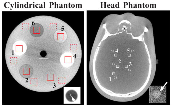
s-ROIs (solid-line squares) and b-ROIs (dashed-line squares) selected within transverse slices at z = 2.0 cm in the cylindrical phantom (left) and z = 1.2 cm in the head phantom (right) for CNR computation. The ROIs in cylindrical phantom correspond to cortical bone (ROI 1 and ROI 4) and breast (ROI 2), brain (ROI 3), liver (ROI 5) and adipose (ROI 6) tissues. The cylindrical and head phantom images are displayed with soft-tissue-grayscale windows of [−257, 143] HU and [−429, 429] HU. The wire insert in the central region of the cylindrical phantom and ROI 2 of the head phantom, which are displayed with a zoomed-in view using grayscale windows of [−1000, −143] HU and [−200, 28] HU, are used as the signals for the detectability calculation. Cupping artifacts can be observed as a result of physical factors, such as beam-hardening and scatter, when the image is displayed with a narrow grayscale window.

C. Image-power-spectrum evaluation

Recognizing the distinction from a true “noise-power spectrum” (NPS) [35]–[37] as useful in the characterization of noise magnitude and correlation in statistically stationary images, we define below a power spectrum (P_c) measured directly from the image reconstruction in otherwise homogeneous ROIs. While P_c dose not strictly obey assumptions of shift invariance and noise stationarity, among others, as the NPS, it provides a useful, quantitative, relative metric of noise magnitude and correlation among the various algorithms for sparse-view reconstruction under consideration. In order to calculate the image fluctuations in a small ROI within a reconstructed image, we select L square-shaped ROIs of equal size at different locations within the image. Each of the ROIs is within the support of the entire image and in the homogeneous region of the image, and each ROI can overlap with other ROI but no more than half of its size. The image-power spectrum on a Cartesian grid is defined as

$$P_c(\mathbf{k})=\frac{1}{L}\sum _{l=1}^L{\mid \text{DFT}\{\mathbf{W}({\mathbf{f}}_l-{\mathbf{f}}_{\mathit{ave}})\}\mid }^2,$$ (9)

where “DFT” denotes the discrete Fourier transform (DFT), k the discrete frequency vector, f_l the image within the l-th ROI, f_ave the mean ROI image and each of its elements represents the average of the values at the same voxel within different ROI images, and W a discrete window function for reducing excessive power at the edges of the ROI [38]. In the evaluation study below, we first calculated image power spectra P_c(k) for selected 2D ROIs and then converted power spectra P_c(k) onto a polar grid, followed by averaging them over the polar angle to obtain power spectra P_p(k) as functions only of discrete radial frequencies k.

D. Detection-task-based evaluation

We also carried out an evaluation study on algorithm performance by using a model observer in a detection task. The detectability index of the model observer is defined as

$${d^{\prime }}^2=\sum _{\mathbf{k}}\frac{{\mid S(\mathbf{k})\mid }^2}{P_c(\mathbf{k})},$$ (10)

where S(k) denotes the DFT of the signal, and P_c (k) the power spectrum of the background. This model observer is similar to the widely used pre-whitening observer, recognizing that analysis from measured data here does not strictly obey the rigorous assumptions of linearity and shift invariance, among others assumes a number of conditions [35], [39], [40], Nevertheless, d′ provides a quantitative metric of relative comparison in task performance among the various sparse-view reconstructions below [37], [41], [42]. Superficially, it appears that CNR and d′ measure similar quantities, but there is a significant difference in how the statistical model of the image enters in these quantities. CNR includes only the estimated image variance in the denominator, while d′ accounts for some measure of the image covariance.

In the study below, the “signal” (i.e., the numerator in Eq. (10)) are the high contrast wire in the cylindrical phantom, highlighted by the small arrow in the square box at the lower-right corner in the left panel of Fig. 2, and the low-contrast, extended tumor in the head phantom, displayed at the lower-right corner in the right panel of Fig. 2. We applied signal masks obtained by using the corresponding FDK-reference images to determining signal regions within reconstructed images. A signal image was subsequently obtained by subtraction from the reconstruction within the determined signal region a background image estimated from a region surrounding the signal region. From the obtained signal image, we subsequently computed the image-energy spectrum S(k). The background power spectra were determined as described in Sec. IV-C above. Using the computed |S(k)|² and P_c(k) in Eq. (10), we then obtained the detectability indices for reconstructed images. The “signal” numerator of Eq. (10) therefore corresponds to spatial-frequency-dependent tasks for (i) detection of the wire, which emphasizes higher frequency structures and (ii) detection of the low-contrast simulated lesion, which emphasizes lower frequency structures.

V. Experimental Study of the cylindrical phantom

For the cylindrical-phantom, we collected full data at 960 views uniformly distributed over 2π. From the full data set, we extracted data sets containing 15, 30, 60, and 96 views evenly distributed over 2π and refer to them as the 15-, 30-, 60-, and 96-view data sets. From the full and sparse-view data sets, images were reconstructed with a voxel size of 0.05 cm. For the ASD-POCS algorithm, the average values of ε per ray measurement were chosen to be about 8.2×10⁻⁶, 5.6×10⁻⁶, 3.9×10⁻⁶ and 3.2×10⁻⁶ for the 15-, 30-, 60-, and 96-view data sets, respectively.

A. Qualitative visual evaluation

Using the FDK, EM, POCS, and ASD-POCS algorithms, we reconstructed images from sparse-view data sets and displayed in Figs. 3 and 4 transverse, sagittal, and coronal images reconstructed from 30- and 60-view data sets, respectively, with bone-and soft-tissue-grayscale windows. As the results show, image differences of different view numbers or different algorithms are more evident when displayed in a narrow grayscale window. In general, images reconstructed with the ASD-POCS algorithm appear visually more similar to the FDK-reference images than the other algorithms.

Figure 3.

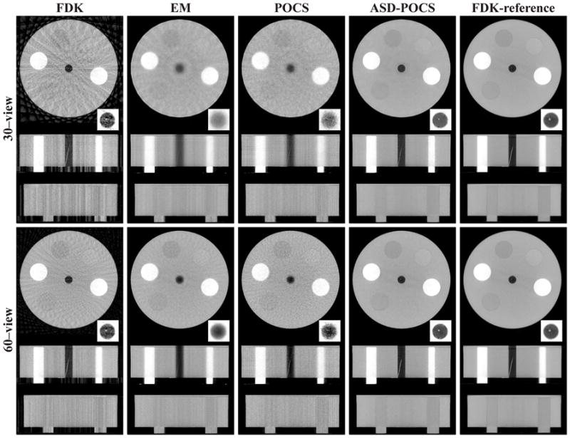
Images of the cylindrical phantom reconstructed from 30-view (rows 1–3) and 60-view (rows 4–6) data sets by use of the FDK, EM, POCS, and ASD-POCS algorithms, within a transverse slice at z = 2.0 cm (rows 1 and 4), coronal slice at x = −3.0 cm (rows 2 and 5), and sagittal slice at y = −0.25 cm (rows 3 and 6). The central region of the transverse slice is redisplayed with a zoomed-in view using a grayscale window of[−1000, −143] HU to show the wire insert. The last column is the FDK-reference images within the corresponding slices. A bone grayscale window, [−1000, 714] HU, is used.

Figure 4.

Images of the cylindrical phantom reconstructed from 30-view (rows 1–3) and 60-view (rows 4–6) data sets by use of the FDK, EM, POCS, and ASD-POCS algorithms, within a transverse slice at z = 2.0 cm (rows 1 and 4), coronal slice at x = −3.0 cm (rows 2 and 5), and sagittal slice at y = −0.25 cm (rows 3 and 6). The central region of the transverse slice is redisplayed with a zoomed-in view using a grayscale window of [−571, −429] HU to show the wire insert. The last column is the FDK-reference images within the corresponding slices. A soft-tissue grayscale window, [−257, 143] HU, is used.

The low-contrast inserts can be distinguished with the number of views as low as 30 for images reconstructed by use of the ASD-POCS algorithm, as shown in Fig. 4. It is also interesting to observe that the high contrast wire in the FOV center was recovered well in both 30- and 60-view FDK-reconstruction images. On the other hand, although the EM and POCS images have less streak artifacts, it is more difficult to observe the wire in the images. This is understandable because the wire is near the FOV center, where it can be sufficiently sampled by a small number of views, thus allowing reasonably accurate FDK reconstruction of the wire. This observation suggests that depending on the task, the FDK algorithm can also perform well when applied to sparse-view data. The wire image obtained with the ASD-POCS algorithm seems to have a contrast level higher than that of the wire in the FDK-reference images, as shown in Fig. 4. It should be noted that, when images are displayed in a narrow grayscale window, some cupping artifacts can be observed that are caused largely by beam-hardening and X-ray scatter.

B. Quantitative-metric-based evaluation

We have also carried out quantitative evaluation studies by using the metrics described in Sec. IV-B.

1) Similarity-metrics evaluation

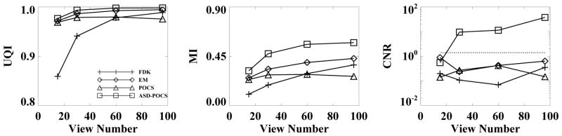
In Fig. 5, we display UQI, and MI computed from reconstructed images of the cylindrical phantom. Also, results similar to those described above were obtained for different ROIs. The results suggest that the ASD-POCS algorithm yields images more similar to the FDK-reference image than do other algorithms under study. The FDK results increase rapidly as the number of views increases. As elaborated in Sec. VII below, this is attributable to the fact that the FDK-reference image was used in the computation of similarity metrics. When the number of views increases, the FDK reconstruction becomes rapidly similar to the FDK-reference image.

Figure 5.

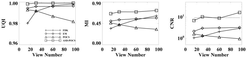
UQI (left), MI (middle), and CNR (right) as functions of projection views, computed from the cylindrical phantom images reconstructed by use of the FDK (+), EM (◇), POCS (△), and ASD-POCS (□) algorithms and the FDK-reference image. The dotted line displays the corresponding CNR in the FDK-reference image.

2) CNR-metric-based evaluation

For the selected s- and b-ROIs in the cylindrical phantom, as shown in Fig. 2, we calculated CNR using Eq. (8) and plot the results, as functions of the projection views in Fig. 5 for pair 6 of s- and b-ROIs, corresponding to the “adipose tissue” inserts. For comparison, we also calculated the CNR for the corresponding ROIs within the FDK-reference image and plot them as the dashed lines. CNR obtained with the ASD-POCS algorithm appears higher than those obtained with other algorithms. This is because the ASD-POCS algorithm generally yields images with a noise level lower than other algorithms under study. Similar CNR results were also obtained for other pairs of s- and b-ROIs in reconstructed images.

3) Image properties as functions of iteration numbers

We also studied the evolution of image reconstruction as functions of iterations in the EM, POCS, and ASD-POCS algorithms. In Fig. 6, we display ROI images containing the low-contrast structures within the slice at z = 0 cm reconstructed from the 60-view data by use of the ASD-POCS algorithm at iterations 2, 10, 30, and 100, with different grayscale windows for showing reconstruction details, Visual inspection of the results suggest that images with reasonable quality can be reconstructed even at early iterations. To assess quantitatively the reconstruction as a function of iterations, we also calculated data divergence, convergence parameter c_α, and quantitative metrics such as UQI and MI for different iterations. The quantitative results, as shown in Fig. 7, corroborate the observation that the ASD-POCS algorithm seems to be able to reconstruct images of reasonable quality at an early stage of the iteration.

Figure 6.

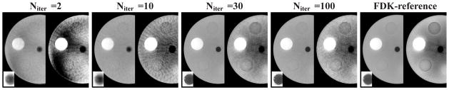
ROI images of the cylindrical phantom within a transverse slice at z = 0 cm reconstructed from 60-view data by use of the ASD-POCS algorithm at iterations 2, 10, 30, and 100. For each displayed iteration number, the ROI image are shown with a bone-grayscale window [−1000, 714] HU (left) and a soft-tissue-grayscale window [−257, 143] HU (right). The square ROI shows the zoomed-in view of the central region containing the wire with a grayscale window [−1000, −143] HU.

Figure 7.

Image-property parameters, as functions of iteration numbers for images reconstructed from 60-view data by use of the ASD-POCS algorithm. Row 1: data divergence D (left) and parameter c_α (right); and row 2: UQI (left) and MI (right) calculated within the entire image support. The dotted line in data-divergence plot indicates the selected ε.

C. Power-spectrum-metric-based evaluation

For the cylindrical phantom experiment, as described in Sec. IV-C, we calculated the power spectra P_p(k) by using 25 40×40 selected ROIs within a 2D image at z = 0 cm and display them in Fig. 8. For comparison, we also calculated the corresponding power spectrum of the FDK-reference image and display it as the dotted curve. The power spectra obtained by use of the FDK, EM, and POCS algorithms agrees well with the reference power spectrum at low frequencies, although the former differs from the latter at high frequencies. This is consistent with the “streakiness” observed in the images. The result of the ASD-POCS algorithm agree well with the reference power spectrum over a frequency range wider than those of the other algorithms.

Figure 8.

Power spectra of the cylindrical phantom obtained from 15-, 30-, 60-, and 96-view data sets by use of the FDK (+), EM (◇), POCS (△), and ASD-POCS (□) algorithms. The power spectrum of the FDK-reference image is plotted as the dotted curve.

D. Detection-task-based evaluation

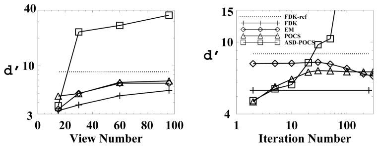
We computed, using Eq. (10), the model-observer detectabilities for the high contrast wire in reconstructed cylindrical-phantom images and display them in Fig. 9 as functions of projection views and iteration numbers. For the latter case, images at different iterations were reconstructed from 60-view data set by use of the EM, POCS, and ASD-POCS algorithms. The results suggest that the ASD-POCS algorithm generally yields a detectability higher than do the other algorithms in terms of the detection task described. We have also computed the detectability indices for reconstructions from other sparse-view data sets, and observations similar to those described above can be made.

Figure 9.

Detectabilities for the wire as functions of projection views (left) and iteration number (right) calculated from cylindrical phantom images reconstructed by use of the FDK (+), EM (◇), POCS (△), and ASD-POCS (□) algorithms. The detectability of the FDK-reference image is plotted as dotted lines.

The following study on a physical head phantom serves as further demonstration and evaluation of the ASD-POCS algorithm, and the complexity of the phantom provides added significant challenge to the constrained TV-minimization.

VI. Experimental study of the anthropomorphic head phantom

For the anthropomorphic head phantom, a full data set was collected at 960 views uniformly distributed over 2π. From the full data set, we extracted data sets containing 15, 30, 60, and 96 views evenly distributed over 2π from which we subsequently reconstructed images with a voxel size 0.045 cm. For the ASD-POCS algorithm, the average values of ε per ray measurement were chosen to be about 3.2×10⁻⁵, 2.4×10⁻⁵, 1.7×10⁻⁵ and 1.3×10⁻⁵ for 15-, 30-, 60-, and 96-view data sets, respectively.

A. Qualitative-visualization-based evaluation

We reconstructed images from the sparse-view data sets of the head phantom and display reconstructions from the 60- and 96-view data sets with a bone- and soft-tissue-grayscale windows in Figs. 10 and 11. The corresponding FDK-reference images are also displayed in the last columns. Observations similar to those for the cylindrical phantom images can be made. Additionally, low-contrast, small spheres mimicking brain tumors in the head phantom can be observed in the transverse and sagittal slices of the FDK-reference image. Although it is difficult to distinguish them in the FDK, EM, and POCS images, they can be discerned in the ASD-POCS reconstructions, suggesting that the ASD-POCS algorithm may not only suppress image artifacts but also retain low-contrast structures. For further visualization of reconstruction details, we show in Fig. 12 the nasal region of the head phantom in a zoomed-in view, using different grayscale windows, reconstructed from 60- and 96-view data. The ASD-POCS algorithm seems to be able to pick up some of the subtle structures that are observed in the FDK-reference image.

Figure 10.

Images of the head phantom reconstructed from 60-view (rows 1–3) and 96-view (rows 4–6) data sets by use of the FDK, EM, POCS, and ASD-POCS algorithms, within a transverse slice at z = 1.2 cm (rows 1 and 4), coronal slice at x = 0.6 cm (rows 2 and 5), and, sagittal slice at y = 2.5 cm (rows 3 and 6). The last column displays the FDK-reference images within the corresponding slices. A bone grayscale window, [−1000, 1000] HU, is used.

Figure 11.

Images of the head phantom reconstructed from 60-view (rows 1–3) and 96-view (rows 4–6) data sets by use of the FDK, EM, POCS, and ASD-POCS algorithms, within a transverse slice at z = 1.2 cm (rows 1 and 4), coronal slice at x = 0.6 cm (rows 2 and 5), and sagittal slice at y = 2.5 cm (rows 3 and 6). The last column displays the FDK-reference images within the corresponding slices. A soft-tissue grayscale window, [−429, 429] HU, is used. Low-contrast tumor structures can be observed in the ASD-POCS reconstructions and FDK-reference images.

Figure 12.

Nasal-region images of the head phantom within a transverse slice at z = 0 cm reconstructed from 60-view (row 1–2) and 96-view (row 3–4) data sets by use of the FDK, EM, POCS, and ASD-POCS algorithms displayed in a bone grayscale window of [−1000, 1000] HU (row 1 and 3) and a soft-tissue grayscale window of [−429, 429] HU (row 2 and 4). The corresponding FDK-reference images are shown in the last column.

B. Quantitative-metric-based evaluation

1) Similarity-metrics-based evaluation

In Fig. 13, we show UQI, and MI, as functions of projection views, computed from reconstructed images of the head phantom. UQI and MI for different ROIs within the head phantom similar to those described above were also obtained. Based upon the results, observations similar to those for the cylindrical phantom can also be made for the head phantom.

Figure 13.

UQI (left), MI (middle) and CNR (right) as functions of projection views, computed from the head phantom images reconstructed by use of the FDK (+), EM (◇), POCS (△), and ASD-POCS (□) algorithms and the FDK-reference image. The dotted line displays the corresponding CNR in the FDK-reference image.

2) CNR-metric-based evaluation

For the selected s- and b-ROIs shown in Fig. 2, we calculated CNR by using Eq. (8). In row 4 of Fig. 13, we display the CNR results as functions of projection views for pair 2 of s- and b-ROIs. For comparison, we also calculated the CNR of the FDK-reference image and plot it as dotted line in Fig. 13. Similar CNR results were also obtained for other pairs of s- and b-ROIs in the head phantom. Again, observations about algorithm performance similar to those for the cylindrical phantom can be made for the head phantom.

3) Image properties as functions of iteration numbers

In Fig. 14, we display ROI images within a transverse slice at z = 0 cm reconstructed using the ASD-POCS algorithm from 96-view data at iterations 2, 10, 30, and 100. The ROI images containing the nasal region that were selected and displayed in a zoomed-view with bone- and soft-tissue-grayscales for revealing reconstruction details. Visual inspection of the images suggest that images with reasonable quality can be reconstructed even at early iterations. We have also calculated data divergence D, convergence parameter c_α, and quantitative metrics UQI and MI at different iterations in which the convergence behavior of the ASD-POCS algorithm similar to that in Fig. 7 can be observed.

Figure 14.

Nasal-region images of the head phantom within a transverse slice at z = 0 cm reconstructed from 96-view data by use of the ASD-POCS algorithm at iterations 2, 10, 30, and 100, displayed with a bone-grayscale window [−1000, 1000] HU (row 1) and a soft-tissue grayscale window [−429, 429] HU (row 2).

C. Power-spectrum-metric-based evaluation

As described in Sec. IV-C, we selected 42 40×40 ROIs within a 2D image at z = 0 cm to calculate the power spectra P_p(k) and display them in Fig. 8. The selected ROIs are within the brain region and have no overlap with the bones in the outer regions of the head. For comparison, the corresponding power spectrum of the FDK-reference image is also displayed as the dotted curve. The general trends of the power spectra obtained for different data sets and different algorithms are consistent with those for the cylindrical phantom.

D. Detection-task-based evaluation

We also computed detectabilities in Eq. (10) for the low-contrast lesion in reconstructed head-phantom images, which are shown in Fig. 16 as functions of projection views and iteration numbers. For the latter case, images at different iterations were reconstructed from 96-view data set. The results suggest that the ASD-POCS algorithm generally yields a detectability higher than do the other algorithms in terms of the detection task described. We have computed detectability indices for reconstructions from other sparse-view data sets, and observations similar to those described above can be made.

Figure 16.

Detectabilities for the low-contrast lesions as functions of projection views (left) and iteration number (right) calculated from head phantom images reconstructed by use of the FDK (+), EM (◇), POCS (△;), and ASD-POCS (□) algorithms. The detectability of the FDK-reference image is plotted as dotted lines.

VII. Comments on the numerical results

The overall summary of the results indicate that image-reconstruction algorithms solving constrained TV-minimization can be effective at significantly reducing streak artifacts when CBCT projections are taken at a limited number of views. The comparisons have been quantified by use of metrics sensitive to different aspects of image quality, and in each case the ASD-POCS algorithm generally yields numbers similar to the FDK-reference image. A notable exception is the MI metric, which measures the histogram correlation between two images. Clearly, it is more sensitive than some other metrics in detecting image differences. For data sets containing more than 30 views, the signal-detection metrics appear to be larger than the FDK-reference. As each of these metrics are ratios of some measure of the reconstructed signal and the image noise, the larger values for CNR and d′ reflect the fact that the signal can be reconstructed while the background is effectively de-noised.

A few words on constrained TV-minimization and the ASD-POCS algorithm are in order. One of the themes of this work is to demonstrate that the optimization problem of constrained TV-minimization, suggested in the CS field, is of interest to image reconstruction with actual CBCT data. The skeptical reader might note that the cylindrical phantom seems to be piecewise constant, and therefore favors the ASD-POCS algorithm for constrained TV-minimization. But we point out that actual scanner data are quite inconsistent with the discrete X-ray transform model of Eq. (1). Streaking and cupping from beam-hardening and X-ray scatter are visible in the FDK-reference image displayed with a soft-tissue grayscale window in Fig. 4. The profiles of the 60-view ASD-POCS, FDK-reference, and ASD-POCS-reference images in Fig. 17 clearly show that the resulting images are not really piece-wise constant.

Figure 17.

Profiles along two lines within the transverse slice at z = 0 cm in the FDK- (dotted curve) and ASD-POCS-reference (solid curve) images and in the 60-view, ASD-POCS reconstruction (dashed curve) of the cylindrical phantom. It is obvious that the images are not piece-wise constant.

Another interesting point, which will take future investigation to clarify, is the question of whether or not the solution to constrained TV-minimization is a desirable image. The plots of D and c_α in Fig. 7 indicate that ASD-POCS is accurately solving Eq. (3). The plots of d′ in Figs. 9 and 16 are quite interesting in addressing this question. Note that, for example, the EM achieves a maximum d′ well short of converging to its minimizer of the KL-data divergence. As an aside, this phenomenon is well-known and is not surprising because we have included no regularization with the EM implementations. (The inclusion of regularizations in the EM algorithm generally leads to a different algorithm that minimizes an objective function that is likely to differ from the pure KL-data divergence that the EM algorithm minimizes.) In contrast, the ASD-POCS algorithm appears to achieve a maximum d′ when the image estimate approaches the solution to Eq. (3). This question is important from the standpoint of the complexity of the image reconstruction. The solution of constrained TV-minimization depends only on data, system matrix, and ε, while intermediate image estimates depend on, in addition to these factors, detailed parameters and implementation of the particular reconstruction algorithm.

The evaluation results can be dependent on a reference image used. In the similarity-metrics-based evaluation studies presented, it is not unreasonable to use the FDK-reference image because it is the image currently used in practical applications. However, the FDK-reference image represents only an approximate reconstruction of the underlying “truth”, and thus the selection of a reference image different from the FDK-reference image is likely to lead to different evaluation results. As shown in Fig. 1, we also include images reconstructed from full, 960-view data by using the ASD-POCS algorithm. These images, which we refer to as the ASD-POCS-reference images, are visually highly similar to the FDK-reference images. However, a close inspection reveals differences between them: the wire in the ASD-POCS-reference image for the cylindrical phantom has higher contrast than that in the FDK-reference image; and more details in the trabecular bone of the head can be observed in the ASD-POCS-reference image than in the FDK-reference image. As shown in row 1 of Fig. 18, the power spectra of the two reference images show some differences at high frequencies. When the ASD-POCS-reference image is used for computing the similarity-based metrics, evaluation results different from those obtained with the FDK-reference image are expected. As an example, MIs computed by using the ASD-POCS-reference images are shown in row 2 of Fig. 18, and it can be observed that they are considerably higher than their counterparts in Figs. 5 and 13 obtained with the FDK-reference images.

Figure 18.

Row 1: Power spectra computed from the FDK-reference (dotted curve) and ASD-POCS-reference (solid curve) images. Row 2: MIs, as functions of projection views, computed from cylindrical (left) and head (right) phantom images obtained by use of the FDK (+), EM (◇), POCS (△), and ASD-POCS (□) algorithms and the ASD-POCS-reference image. They differ from their counterparts in Figs. 5 and 13, which were obtained with the FDK-reference images.

The results shown bear certain information of spatial resolution in reconstructions. However, some widely used tools such as the modulation transfer function (MTF) for image-resolution evaluation may not be meaningfully defined for the cases under study due not only to gross violations of linearity and shift-invariance but also because an iterative algorithm is based generally on a discrete imaging model in which the system matrix depends on the data-array size and the image-array size. The use of different image-array sizes leads to different system matrices and, consequently, to essentially different optimization problems. Depending upon the selected sizes of an image array and the associated voxels, the optimization problem can become highly under-determined and thus result in distinct reconstructions. Therefore, schemes and metrics for the evaluation of spatial resolution in linear, analytic reconstructions may not simply be applied to nonlinear, iterative reconstructions. Some of the evaluation studies were carried out based upon ROI images within selected 2D slices in 3D reconstructions. We have also performed such evaluation studies in 3D ROI images and obtained evaluation results similar to those described above.

VIII. Discussion

The work focuses on imaging configurations consisting of flat-panel detector and circular scanning trajectory, which are the most widely adopted imaging configurations in non-diagnostic CT. The ASD-POCS algorithm can readily be applied to imaging configurations of curved or spherical detector and non-circular scanning trajectories such as helical trajectory. There are other issues worthy of future studies, which the ASD-POCS algorithm can also be tailored to tackle. In the study, we considered image reconstruction only from data collected at uniformly distributed sparse views. We investigated an efficient form of ASD-POCS image reconstruction from real data collected in breast tomosynthesis in which the scanning angle (≈ 20°) is severely limited [30]. However, CT imaging involving angular ranges of 100°–180° may find a wide variety of applications. Therefore, investigation of image reconstruction from real data collected from such angular ranges should bear considerable practical significance. Furthermore, in the study reported here, the signal-to-noise (SNR) ratios at each view in both sparse-view and full data sets remain comparable. As such, the total radiation dose in a sparse-view data set is only a small fraction of that in the full data set. It is also of practical significance to investigate image reconstruction as a function of the view number, and the SNR level at each view, in real data studies.

A complete iteration in the ASD-POCS algorithm consists of forward/backward projections and image-TV computations and, as such, of more than twice of the number of computation operations in the FDK. Therefore, the computation time of the ASD-POCS with N iterations can be more than 2N times longer than that of the FDK. In contrast, the forward/backward projections within a complete iteration in the ASD-POCS, POCS, and EM are comparable, but the ASD-POCS involves additional TV-minimization computations. The computation speed of the ASD-POCS algorithm can be enhanced substantially through streamlining/parallelizing its implementation and/or by exploiting the available, or rapidly available, high performance computational hardware such as multi-core CPU, graphic processing unit (GPU) [43], and cell engines [44]. Although most of the computation results presented were obtained with more than 100 iterations, depending upon imaging conditions and application tasks, it is possible that images obtained at iteration numbers (e.g., ~ 10) much smaller than 100 can be of sufficient practical utility, as evidenced by the visualization-based and quantitative-metrics-based results presented. It is of worthy to point out that the ASD-POCS provides a framework for solving a constraint optimization problem. In the study, the POCS-step employs, e.g., the POCS for lowering the data divergence. However, other appropriate algorithms such as simultaneous algebraic reconstruction technique (SART) [45] and gradient descent can also be used.

As mentioned above, algorithms different from the EM, POCS, and ASD-POCS may be derived for solving the corresponding unconstrained and constrained optimization formulations under consideration. Moreover, one can design different optimization formulations and derive reconstruction algorithms specifically for solving the formulations. These algorithms are worthy of future investigation.

IX. Conclusion

The current work demonstrates and evaluates the potential and robustness of constrained TV-minimization and the ASD-POCS algorithm in image reconstruction of potential utility from real data, collected in CBCT experiments, which contain realistic physical factors that may not be included in simulation studies. To evaluate the multiple facets of image quality, the study consisted of several levels of analysis for revealing different aspects of reconstruction properties, ranging from visual inspection to quantitative-metric-based analysis to detection-task-based assessment. Results of the study demonstrate that, for the imaging conditions, including X-ray flux and data calibration, under consideration, the ASD-POCS algorithm consistently reconstructs images of quality comparable to that of the FDK-reference image from data that are much less than the full data currently used. These results demonstrate the potential for reconstruction approaches and algorithms, such as the constrained TV-minimization and the associated ASD-POCS algorithm, to yield high image quality at significantly reduced view sampling. The implication for dose reduction suggests a potentially important role for such approaches in the future of CT applications.

Figure 15.

Power spectra of the head phantom obtained from 15-, 30-, 60-, and 96-view data sets by use of the FDK (+), EM (◇), POCS (△), and ASD-POCS (□) algorithms. The power spectrum of the FDK-reference image is plotted as the dotted curve.

References

- 1.Brenner DJ, Hall EJ. Computed tomography–an increasing source of radiation exposure. N Engl J Med. 2007;357:2277–2284. doi: 10.1056/NEJMra072149. [DOI] [PubMed] [Google Scholar]
- 2.De Gonzalez AB, Mahesh M, Kim K, Bhargavan M, Lewis R, Mettler F, Land C. Projected cancer risks from computed tomographic scans performed in the United States in 2007. Arch Intern Med. 2009;169:2071–2077. doi: 10.1001/archinternmed.2009.440. [DOI] [PMC free article] [PubMed] [Google Scholar]
- 3.Smith-Bindman R, Lipson J, Marcus R, Kim K, Mahesh M, Gould R, de Gonzalez AB, Miglioretti DL. Radiation dose associated with common computed tomography examinations and the associated lifetime attributable risk of cancer. Arch Intern Med. 2009;169:2078–2086. doi: 10.1001/archinternmed.2009.427. [DOI] [PMC free article] [PubMed] [Google Scholar]
- 4.Feldkamp LA, Davis LC, Kress JW. Practical cone-beam algorithm. J Opt Soc Am A. 1984;1:612–619. [Google Scholar]
- 5.Katsevich A. Theoretically exact filtered backprojection-type inversion algorithm for spiral CT. SIAM J Appl Math. 2002;62:2012–2026. [Google Scholar]
- 6.Zou Y, Pan X. Exact image reconstruction on PI-lines from minimum data in helical cone-beam CT. Phys Med Biol. 2004;49:941–959. doi: 10.1088/0031-9155/49/6/006. [DOI] [PubMed] [Google Scholar]
- 7.Pack JD, Noo F, Clackdoyle R. Cone-beam reconstruction using the backprojection of locally filtered projections. IEEE Trans Med Imag. 2005;24:70–85. doi: 10.1109/tmi.2004.837794. [DOI] [PubMed] [Google Scholar]
- 8.Brooks RA, Glover G, Talbert AJ, Eisner RL, DiBianca FA. Aliasing: A source of streaks in computed tomograms. J Comput Assist Tomogr. 1979;3:511–518. [PubMed] [Google Scholar]
- 9.Crawford CR, Kak AC. Aliasing artifacts in computerized tomography. Applied Optics. 1979;18:3704–3711. doi: 10.1364/AO.18.003704. [DOI] [PubMed] [Google Scholar]
- 10.La Riviere PJ, Pan X. Few-view tomography using roughness-penalized nonparametric regression and periodic spline interpolation. IEEE Trans Nucl Sci. 1999;46:1121–1128. [Google Scholar]
- 11.Galigekere RR, Wiesent K, Holdsworth DW. Techniques to alleviate the effects of view aliasing artifacts in computed tomography. Med Phys. 1999;26:896–904. doi: 10.1118/1.598606. [DOI] [PubMed] [Google Scholar]
- 12.Delaney A, Bresler Y, Sunnyvale C. Globally convergent edge-preserving regularized reconstruction: an application to limited-angle tomography. IEEE Trans Image Process. 1998;7:204–221. doi: 10.1109/83.660997. [DOI] [PubMed] [Google Scholar]
- 13.Loose S, Leszczynski KW. On few-view tomographic reconstruction with megavoltage photon beams. Med Phys. 2001;28:1679–1688. doi: 10.1118/1.1387273. [DOI] [PubMed] [Google Scholar]
- 14.Li M, Yang H, Kudo H. An accurate iterative reconstruction algorithm for sparse objects: application to 3D blood vessel reconstruction from a limited number of projections. Phys Med Biol. 2002;47:2599–2609. doi: 10.1088/0031-9155/47/15/303. [DOI] [PubMed] [Google Scholar]
- 15.Candés E, Romberg J, Tao T. Robust uncertainty principles: exact signal reconstruction from highly incomplete frequency information. IEEE Trans Inf Theory. 2006;52:489–509. [Google Scholar]
- 16.Candès E, Romberg J, Tao T. Stable signal recovery from incomplete and inaccurate measurements. Commun Pure Appl Math. 2006;59:1207–1223. [Google Scholar]
- 17.Sidky EY, Kao KM, Pan X. Accurate image reconstruction from few-views and limited-angle data in divergent-beam CT. J X-Ray Sci and Technol. 2006;14:119–139. [Google Scholar]
- 18.Sidky EY, Pan X. Image reconstruction in circular cone-beam computed tomography by constrained, total-variation minimization. Phys Med Biol. 2008;53:4777–4807. doi: 10.1088/0031-9155/53/17/021. [DOI] [PMC free article] [PubMed] [Google Scholar]
- 19.Sidky E, Anastasio M, Pan X. Image reconstruction exploiting object sparsity in boundary-enhanced X-ray phase-contrast tomography. Opt Express. 2010;18:10 404–10 422. doi: 10.1364/OE.18.010404. [DOI] [PMC free article] [PubMed] [Google Scholar]
- 20.Candès E, Wakin MB. An introduction To compressive sampling. IEEE Signal Process Mag. 2008;25:21–30. [Google Scholar]
- 21.Dempster AP, Laird NM, Rubin DB. Maximum likelihood from incomplete data via the EM algorithm. J R Stat Soc Series B Stat Methodol. 1977;39:1–38. [Google Scholar]
- 22.Shepp LA, Vardi Y. Maximum likelihood reconstruction for emission tomography. IEEE Trans Med Imag. 1982;1:113–122. doi: 10.1109/TMI.1982.4307558. [DOI] [PubMed] [Google Scholar]
- 23.Gordon R, Bender R, Herman GT. Algebraic reconstruction techniques (ART) for three-dimensional electron microscopy and X-ray photography. J Theor Biol. 1970;29:471–481. doi: 10.1016/0022-5193(70)90109-8. [DOI] [PubMed] [Google Scholar]
- 24.Youla DC, Webb H. Image restoratoin by the method of convex projections: Part 1 – theory. IEEE Trans Med Imag. 1982;1:81–94. doi: 10.1109/TMI.1982.4307555. [DOI] [PubMed] [Google Scholar]
- 25.Combettes PL. The foundations of set theoretic estimation. in Proc IEEE. 1993;81:182–208. [Google Scholar]
- 26.Tward DJ, Siewerdsen JH. Cascaded systems analysis of the 3D noise transfer characteristics of flat-panel cone-beam CT. Med Phys. 2008;35:5510–5529. doi: 10.1118/1.3002414. [DOI] [PMC free article] [PubMed] [Google Scholar]
- 27.Chiarot CB, Siewerdsen JH, Haycocks T, Moseley DJ, Jaffray DA. An innovative phantom for quantitative and qualitative investigation of advanced X-ray imaging technologies. Phys Med Biol. 2005;50:N287–N297. doi: 10.1088/0031-9155/50/21/N01. [DOI] [PubMed] [Google Scholar]
- 28.Barrett HH, Myers KJ. Foundations of Image Science. John Wiley Sons, Inc; 2003. [Google Scholar]
- 29.Pan X, Sidky EY, Vannier M. Why do commercial CT scanners still employ traditional, filtered back-projection for image reconstruction? Inverse Probl. 2009;25:123009. doi: 10.1088/0266-5611/25/12/123009. [DOI] [PMC free article] [PubMed] [Google Scholar]
- 30.Sidky EY, Pan X, Reiser IS, Nishikawa RM, Moore RH, Kopans DB. Enhanced imaging of microcalcifications in digital breast tomosynthesis through improved image-reconstruction algorithms. Med Phys. 2009;36:4920–4932. doi: 10.1118/1.3232211. [DOI] [PMC free article] [PubMed] [Google Scholar]
- 31.Leng S, Tang J, Zambelli J, Nett B, Tolakanahalli R, Chen GH. High temporal resolution and streak-free four-dimensional cone-beam computed tomography. Phys Med Biol. 2008;53:5653–5673. doi: 10.1088/0031-9155/53/20/006. [DOI] [PMC free article] [PubMed] [Google Scholar]
- 32.Herman GT, Davidi R. Image reconstruction from a small number of projections. Inverse Probl. 2008;24:045011. doi: 10.1088/0266-5611/24/4/045011. [DOI] [PMC free article] [PubMed] [Google Scholar]
- 33.Wang Z, Bovik A. A universal image quality index. IEEE Signal Process Lett. 2002;9:81–84. [Google Scholar]
- 34.Pluim JPW, Maintz JBA, Viergever MA. Mutual-information-based registration of medical images: a survey. IEEE Trans Med Imag. 2003;22:986–1004. doi: 10.1109/TMI.2003.815867. [DOI] [PubMed] [Google Scholar]
- 35.Burgess AE, Judy PF. Signal detection in power-law noise: effect of spectrum exponents. J Opt Soc Am A. 2007;24:B52–B60. doi: 10.1364/josaa.24.000b52. [DOI] [PubMed] [Google Scholar]
- 36.Metheany KG, Abbey CK, Packard N, Boone JM. Characterizing anatomical variability in breast CT images. Med Phys. 2008;35:4685–4694. doi: 10.1118/1.2977772. [DOI] [PMC free article] [PubMed] [Google Scholar]
- 37.Gang GJ, Tward DJ, Lee J, Siewerdsen JH. Anatomical background and generalized detectability in tomosynthesis and cone-beam CT. Med Phys. 2010;37:1948–1965. doi: 10.1118/1.3352586. [DOI] [PMC free article] [PubMed] [Google Scholar]
- 38.Percival DB, Walden AT. Spectral Analysis for Physical Applications. Cambridge University Press; New York: 1993. [Google Scholar]
- 39.International Commission on Radiation Units and Measurements. Tech Rep ICRU Report No 54. Bethesda, MD: 1996. Medical image–the assessment of image quality. [Google Scholar]
- 40.Burgess AE, Jacobson FL, Judy PF. Human observer detection experiments with mammograms and power-law noise. Med Phys. 2001;28:419–437. doi: 10.1118/1.1355308. [DOI] [PubMed] [Google Scholar]
- 41.Siewerdsen JH, Jaffray DA. Optimization of X-ray imaging geometry (with specific application to flat-panel cone-beam computed tomography) Med Phys. 2000;27:1903–1914. doi: 10.1118/1.1286590. [DOI] [PubMed] [Google Scholar]
- 42.Reiser IS, Nishikawa RM. Task-based assessment of breast tomosynthesis: Effect of acquisition parameters and quantum noise. Med Phys. 2010;37:1591–1600. doi: 10.1118/1.3357288. [DOI] [PMC free article] [PubMed] [Google Scholar]
- 43.Xu F, Mueller K. Accelerating popular tomographic reconstruction algorithms on commodity PC graphics hardware. IEEE Trans Nucl Sci. 2005;52:654–663. [Google Scholar]
- 44.Kachelrieß M, Knaup M, Bockenbach O. Hyperfast parallel-beam and cone-beam backprojection using the cell general purpose hardware. Med Phys. 2007;34:1474–1486. doi: 10.1118/1.2710328. [DOI] [PubMed] [Google Scholar]
- 45.Andersen AH, Kak AC. Simultaneous algebraic reconstruction technique (SART): a superior implementation of the ART algorithm. Ultrason imaging. 1984;6:81–94. doi: 10.1177/016173468400600107. [DOI] [PubMed] [Google Scholar]