Extracting Fuzzy Classification Rules from Texture Segmented HRCT Lung Images

Abstract

Automatic tools for detection and identification of lung and lesion from high-resolution CT (HRCT) are becoming increasingly important both for diagnosis and for delivering high-precision radiation therapy. However, development of robust and interpretable classifiers still presents a challenge especially in case of non-small cell lung carcinoma (NSCLC) patients. In this paper, we have attempted to devise such a classifier by extracting fuzzy rules from texture segmented regions from HRCT images of NSCLC patients. A fuzzy inference system (FIS) has been constructed starting from a feature extraction procedure applied on overlapping regions from the same organs and deriving simple if–then rules so that more linguistically interpretable decisions can be implemented. The proposed method has been tested on 138 regions extracted from CT scan images acquired from patients with lung cancer. Assuming two classes of tissues C1 (healthy tissues) and C2 (lesion) as negative and positive, respectively; preliminary results report an AUC = 0.98 for lesions and AUC = 0.93 for healthy tissue, with an optimal operating condition related to sensitivity = 0.96, and specificity = 0.98 for lesions and sensitivity 0.99, and specificity = 0.94 for healthy tissue. Finally, the following results have been obtained: false-negative rate (FNR) = 6 % (C1), FNR = 2 % (C2), false-positive rate (FPR) = 4 % (C1), FPR = 3 % (C2), true-positive rate (TPR) = 94 %, (C1) and TPR = 98 % (C2).

Introduction

Clinical outcome of radiotherapy can potentially be improved by increasing the precision of tumor localization and dose delivery during the treatment. The size of the necessary margins, and hence the risk for complications, can be reduced if the setup uncertainties and internal organ motion, such as those caused by breathing motion, are minimized. For this to happen, it is necessary to know the shape and the location of the tumor and organs at risk (OAR) at the time of delivery. It has been shown in the past that four-dimensional CT (4DCT) offers the potential for online dynamic multileaf collimator-based respiratory motion tracking; however, there is lack of proper tools [1]. Four-dimensional treatment can be defined as the explicit inclusion of the temporal changes in anatomy during the planning, imaging, and delivery of radiotherapy [2]. As the amount of images to be processed can vary in hundreds, tools for automated detection and identification of pathologic lung tissue patterns are an essential first step towards high-precision image-guided radiation therapy (IGRT). When the chest x-rays do not carry enough elements to finalize the diagnosis, high-resolution computed tomography (HRCT) is used to provide an accurate assessment of lung tissue patterns [3]. Many methods have been developed and tested on a wide range of applications for automated segmentation and detection in medical imaging. Uncertainties in radiation treatment have been mainly accounted for the delineation of the target volume and physiological motion of the organs for example due to patient breathing. Previous approaches to address these uncertainties are discussed below and then a brief rationale for the current study is presented.

1. Previous approaches for lesion delineation:

   For a long time [4], the definition of target volumes was recognized as one of the first uncertainties encountered in planning radiotherapy treatments. The definition of gross tumor volume (GTV) was neglected somewhat as the general idea was that GTV can be reasonably defined as compared to the clinical target volume [4–6]. Incited by the data from Leunens [7], it became clear that defining gross tumor volume is not simple and there might be a risk of over reliance on the physicians’ capabilities of estimating the tumor extent from imaging modalities [8]. Due to a number of uncertainties and tumor-related phenomenon, GTV definition in thoracic radiotherapy could result in larger variations of volumes and dimensions [6–9]. Many attempts have been made since for comparing the GTV as delineated by radiation oncologists, radiologists (with varied experience and expertise) [10–12], and software-based detection, delineation, and identification [13–15]. These methods have reported an accuracy of approximately 90 %. Recent surveys [16, 17] with evaluations of different methods yielded sensitivities between 70 and 90 % with a false positive of 0.5 to 15 per scan.

   Most of these approaches, although beginning with a semi-automatic or manual delineation of suspicious tissue mass, succeed in representing abnormality. In our previous approach [18], we have developed a fully automated delineation and recognition system based upon texture properties of the tissues in lung CT.

   We have introduced class redundancies for GTV (i.e., classes lesion innermost core (LEIN1), lesion inner periphery (LEIP), lesion outer periphery (LEOP) taken together make the GTV) in order to track lung tumor while the patient breathes freely. The approach reached sensitivities of 0.895 with a simple support vector machine (SVM) classifier but at the cost of an high false alarm rate (14.8 %).

1. Previous approaches for lung tumor tracking:

   Lung tumor tracking can be generally categorized as direct tumor tracking, tracking via breathing surrogates, or tracking of implanted fiducial markers. Tracking based upon implanted fiducial markers have been investigated by [19, 20] and is shown to be quite accurate. Two significant drawbacks of implanted marker tracking are risks of clinical complications such as pneumothorax [21, 22] and appealing as well-chosen surrogate can be easily tracked; however, it has been shown that correlation of surrogate motion with the tumor motion may vary with time and require periodic validation [23, 24]. The problems relating to marker- and surrogate-based tracking can be avoided by markerless tracking. Accurate markerless tracking is much difficult to achieve since tumors lack sufficient contrast or a clear border and can be difficult to delineate. In addition, the clinician has to define tumor positions in many images for model making and training purposes.

   The present study is made in order to reduce the false-positive rate and to understand the underlying rules governing automatic tumor recognition by designing if–then-based fuzzy classifier. Such a classifier can be used for (1) tracking in a 4DCT sequence for building patient-specific breathing motion model (See Fig. 1) and (2) as a second opinion for radiologists in the clinics for detecting pulmonary nodules.

   Despite these efforts, it remains a daunting task for the system designer to decide which approach is suited for a particular segmentation task. In addition, uncertainties are widely present in the image data because of the noise in acquisition and of the partial volume effects originating from the low resolution of sensors. In particular, borders between tissues are not exactly defined and memberships in the boundary regions are intrinsically fuzzy. Several artificial intelligence techniques including neural networks and fuzzy logic systems have been successfully applied to a variety of decision-making process in medical diagnosis [25]. Rule-based expert systems are often applied to classification problems in fault detection, biology, medicine, etc. Fuzzy logic improves classification and decision support systems by allowing the use of overlapping class definitions and improves the interpretability of the results by providing more insight into the classifier structure and decision-making process.

   In order to improve the performance of the classifier and in addition look for hidden rules relating the features and decisions, in this paper, we look at fuzzy classification approach in order to classify texture-based segmented regions by using simple if–then fuzzy rules so that more linguistically interpretable decisions can be implemented. Due to texture delineation, our dataset is composed of regions from the same organ or tissue mass. Consequently, it would be more intuitive to use a fuzzy classifier for better labeling of the regions as delineated by texture segmentation [18]. The main advantage of fuzzy rule-based systems is that they do not require large memory storage, their inference speed is very high and users of the system can carefully examine the rule base.

Fig. 1.

Components of tumor tracking from image sequence

Materials

The CT scans were acquired from patients with lung cancer at the Institute of Cancer Research, Oslo University Hospital, Montebello, Norway. The CT scan images were acquired on a four-slice CT scanner (GE) and a single slice CT scanner (GE) equipped with fluoroscopy functionality. Some of the images are acquired during fluoroscopy-guided biopsy, while others are acquired as part of a diagnostic examination and some are acquired during radio frequency ablation (RFA). For images acquired from diagnostic examination, we have used a LightSpeed QX/i4 slice CT scanner with pitch of 1.5, slice thickness of 2.5 mm, in helical mode. For fluoroscopy-guided biopsy and RFA, HiSpeed CT/i was used with slice thickness 3 mm, pitch 0, and helical mode. Images are stored in DICOM (Digital Communication and Imaging in Medicine) format 512 × 512 pixels and with 12-bit gray level depth and the images were anonymized and exported from PACS (Agfa).

The number of images analyzed was 41. Using the same dataset considered in [18], 12 different kinds of tissues are identified: left lung upper or inner part (LLUP), left lung lower part (LLLO), left lung inner periphery (LLIP), left lung outer periphery (LLOP), right lung upper or inner part (RLUP), right lung lower part (RLLO), right lung inner periphery (RLIP), right lung outer periphery (RLOP), lesion innermost core (LEIN1), lesion outer periphery (LEOP1), lesion inner periphery (LEIP1), and BACK (background region). A graphical example is reported in Fig. 2. The lesions were pre-marked by expert radiologists who manually segmented the images. The 41 images have been also automatically segmented following the procedure described in [18], based on fuzzy C-means clustering initialized using genetic algorithm. Then, starting from the automatically segmented regions, a portion for each of the previous mentioned classes is extracted. Given that in the presented study we do not consider the background tissue that causes a dangerous data unbalance, the 11 features described in [18] are then computed on the 11 different portions of the lung, leading to a total number of 393 features vectors. Among them, 138 vectors are used for testing while the remaining 255 are used for training the system. Specifically, Table 1 reports a detailed description of the training set used in our work.

Fig. 2.

Examples of automatically segmented lung tissue

Table 1.

Number of portions extracted for the training and test sets

 

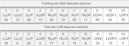
Considering the limited number of images and the consequent increasing difficulty arising in developing a multilabels classification system, this preliminary study is only devoted to the study of the binary problem associated to the classification of the lung portions into healthy (class C1 including classes 1–8) and lesion tissue (C₂ including classes 9–11).

The lesions were pre-marked by expert radiologists. The lesions were of type non-small cell lung cancer (adenocarcinomas) with 3–30.6 mm range including multiple lung metastases. Malignancy has been proved by biopsy. Subtlety of the lesions was not given and consequently this information has not been used in this study. The location of tumors was on the periphery of the chest wall as well as in the lobular regions of the lung. The slice thickness of the CT scan was 2.5 mm. Studies by Stevens et.al. [26] have shown that respiratory-driven lung tumor motion is independent of tumor size, location, and pulmonary function of the patient. We have not conducted any studies as yet on this issue. The average age of patients analyzed was 64 years (max = 86, min = 46, std = 11). However, it is not clear if age has any effect as the variation in age between patients were quite substantial. This aspect has not been taken into account in this study.

Background

IGRT has the potential for distributing continuous delivery of radiation provided the tumor and OAR-like lung can be tracked as the patient breathes freely. Tracking can further be used for tumor motion modeling [18, 27].

For this to be feasible, as a prerequisite, we need tools that can automatically detect and identify the tumor as the patient breathes freely. Figure 1 represents the different steps involved in tumor tracking which are used for model building [18]. First, images from patients with non-small cell lung carcinoma are automatically segmented and a classifier is trained for automatic identification of regions pertaining to lung and lesion [28]. This classifier is then used upon a 4DCT image sequence of a patient for tracking the tumor as the patient breathes freely. Finally, a full breathing cycle of tracked tumor image sequences are co-registered for determining the tumor motion model parameters specific to the patient [18]. In case the classifier is not robust, this can lead to miss the lesion identification from the respiratory cycle thereby producing a suboptimal model. Thus, in this paper, we have addressed the important problem of lesions classification from HRCT images of different patients. In a previous work [28], the authors have attempted an unsupervised detection and classification system for lung and lesion. Although the automatic detection system was good, it was observed that the recognition part often produced high false alarm. The false-positive rate in paper quoted [18] was 14.8 %.

In this paper, we further improve upon the classifier design by extracting fuzzy rules from texture segmented regions. Our aim here is to determine the underlying rule-based structure which increases the radiologist’s interpretability of the results. Fuzzy logic was introduced by Zadeh [29] in 1965 for handling uncertain and imprecise knowledge in real-world applications. Since then, it has found many applications in decision-making tasks and handling of noisy data. The central notion to fuzzy systems is that a variable belongs to a certain set with a membership degree on the range [0; 1], thus relaxing the classic statement that the membership of an element to a set is a binary number. The way the system aggregates variables is then a rule-based inference mechanism very similar to the human language and reasoning. The rules are derived by expert knowledge or by large populations data. Each rule is usually encoded in the form of “IF–THEN” rules. The fuzzy inference system (FIS) we consider is not developed according to classical fuzzy logic theory, but starting from the FIS for medical diagnosis firstly described in [30]. This kind of FIS has been already applied in the automatic identification of breast masses [31], in the malignancy assessment of clusters of calcifications [32] in mammography, and in the development of a novel scoring system for patients in intensive care units [33].

Method

The classification problem is usually modeled [30] by considering three fuzzy sets: patients’ set, diagnoses’ set, and symptoms’ set. Since the considered segmentation problem is solved within a classification framework, then the term diagnoses will be substituted by classes in the following:

1. Patients’ set. In our work, the patient is represented by each portion extracted in the CT lung image. In the following, we will denote it with I.

2. Classes’ set. In this context, classes are represented by the 12 different types of regions encountered in the segmentation process, identified with LLUP, LLLO, LLIP, LLOP (left lung parts), RLUP, RLLO, RLIP, RLOP (right lung parts), LEIN1, LEOP1, LEIP1 (lesion inner and outer parts), and BACK (background region), described in Section 2. Let us identify generically the classes with C_i, i = 1, … ,12. In particular, as already mentioned, in this preliminary work, we will reduce the multiclass problem into a binary classification problem, by merging classes from 1 to 8 into class C₁ and classes from 9 to 11 into class C₂. Class 12 represents regions which are not related to lung and lesion and therefore have been excluded from our analysis. Classes 1–8 refer to healthy tissues pertaining to the left and right lung of the patient whereas classes 9–11 correspond to lesion. As we want to design a binary classifier capable to differentiate between healthy lung tissue and lesion, such a merging of classes is most intuitive.

3. Symptoms’ set. Symptoms in classification problem are usually addressed as features. In this work, we will consider quantitative features extracted from the digital images through a dedicated processing system.

Referring to [30], we only emphasize that a FIS system allows to consider also qualitative or compound features (mixed qualitative and quantitative), expressing them by linguistic terms. However, in this study, we will consider only the 11 quantitative features also described in [18] extracted on the segmented CT image and denoted with eccentricity (F₁), ratio (F₂), complexity (F₃), solidity (F₄), orientation (F₅), number of holes (F₆), mean (F₇), variance (F₈), centroid X (F₉), and Y (F₁₀), area (F₁₁). We will identify the symptoms with F_k, k = 1, … ,11.

The assignment of a class to the considered portion I consists of the evaluation of three distinct relations:

1. Relation image–features (I–F). This relationship describes and quantifies the presence of a feature in the portion of the image under test. The result of this relation is a membership degree assigned as explained in Section 4.1.

2. Relation feature–class (F–C). This relationship quantifies the a priori significance of the feature for the specific class. Still, in this step, the system offers several possibilities to proceed. The operator may manually set the significance of the parameter for a certain class based on the experience of the physician, or the system can detect it automatically from the training set. In this second case, the system can calculate for example the area under the receiving operating curve (ROC) associated with each parameter for each class or it can calculate an alternative significance that also takes account of the prevalence of the class considered. This approach will be described in detail in the following paragraphs. Having in mind that from a medical perspective a symptom may be significant for two or more diagnoses simultaneously, or, on the contrary, not be significant for both of them, it could be interesting to have an approach that establishes the significance of a feature for each class independently.

3. Relation image–class (I–C). This relationship assigns to the selected portion the membership degree to each class, according to the two previous relations.

Formally, denoting with C_i the ith class, with I_j the jth portion, and with F_k the kth feature, then a possible rule is:

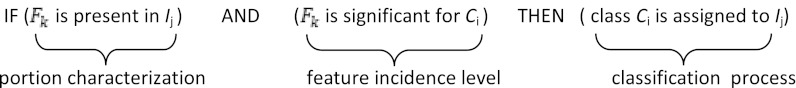
Note that this fuzzy inference rule emulates the physician’s diagnosis inference process in assigning a diagnosis (class) to a patient (portion of the lung tissue) after observing and measuring the patient’s symptoms (portion features) and using his/her experience concerning the influence that a feature has on a certain diagnosis (features incidence level for a class extracted from the portion features computed on a training set). Let us describe in more detail how the proposed FIS implements the two processes: portion characterization and the feature incidence level computation.

Implementation of the Portion Characterization Procedure

The tissue portion characterization procedure assigns to each feature F_k two fuzzy sets, denoted as LOW and HIGH in the following, deriving two membership functions (MFs) and from the histogram of each feature for the different classes. This procedure is usually referred as input fuzzification. As already noted, this paper addresses a binary problem in which the 11 classes are grouped into two classes: healthy lung tissue (C₁) which needs to be protected from unnecessary irradiation and lesion (C₂) where a lethal dose is to be delivered with precision. This assumption implies the construction of the histogram of F_k for two classes. The histogram of a feature represents the distribution of the feature values on a certain population and constitutes the knowledge base for the algorithm. Figure 3 represents an example of the MFs construction for feature F₄.

Fig. 3.

Construction of the MFs LOW and HIGH for feature solidity

We used manual contouring from expert radiologist for the validation of the lesion segmentation (see [18]). As our system is based upon fully automatic segmentation and feature extraction, the only input to be provided to the system is the CT image of the patient. The study takes into account multiple lesions from the same patient including metastasis. It treats, however, each finding as independent. There is no relationship between multiple findings. Detailed steps are summarized in the block diagram shown in Fig. 4 for a generic feature F_k acquired on a certain population whose members belong to the class C₁ or C₂. The flowchart describes how to assign to a measured value F_k a membership degree representing how much the feature is present in that image, separately for the two classes. In fact, considering again Fig. 4, the procedure can lead to four different cases according to the feature distribution over the two classes:

• Case 1. Low values of F_k are related to class C₁ and high values to class C₂;

• Case 2. Low values of F_k are related to class C₂ and high values to class C₁;

• Case 3. Low values and high values of F_k are related to class C₁ while there are not significant values of F_k related to class C₂;

• Case 4. Low values and high values of F_k are related to class C₂ while there are not significant values of F_k related to class C₁.

Fig. 4.

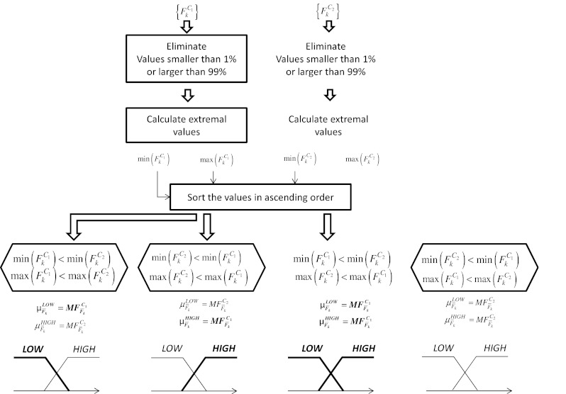
A flowchart representing the fuzzy inference system

Concerning the MFs expression, in this work, we assume triangular-shaped MFs. As shown in Fig. 4, after the evaluation of the extremal values of the feature F_k for both the classes, , a vector containing the ordered extremal values is constructed. Denote with a and b the second and third element of this vector. Then, we get

Implementation of the Feature Influence Level Evaluation

The second antecedent of the fuzzy rule is strictly related to the available knowledge about the influence of a feature on each class. It is a non-standard procedure in fuzzy inference system, but it strictly related to the FIS for medical diagnosis proposed in [30]. In this context, we call this quantity influence level and we denote it as , i = 1,2. It is similar to the evaluation of the significance of a feature computing its area under the ROC (AUC) in a binary pattern classification problem. Recall that, the AUC of a feature is a numerical value representing the area under the ROC of that feature for a certain class in a binary classification process. It is in the range [0, 1] and quantifies how discriminant is that feature alone for the classification problem considered. In particular, considering a varying cut-off ranging from the minimum to the maximum values of the feature, and using this value as discriminated against for the two classes, the ROC plots the true-positive rate (TPR) in respect of the false-positive rate (FPR). Ideally, the AUC is equal to 1 when there is a totally discriminant cut-off value for that feature that separate members of the positive class from those of the negative class.

This approach does not take account of the prevalence of one class over another, and nor does the possibility that a symptom is very significant for a class and nothing for the other class.

There are important differences among the AUC evaluation and the method presented in this paper. The influence of a feature is evaluated separately on each class and there is not any complementary between the two influence levels of a feature on the two classes. Let us explain the method with more details.

Considering again the flowchart in Fig. 4, there can be two degenerate situations: in case 3, the incidence level of feature F_k for class C₂ is zero and in case 4, the incidence level for class C₁ is zero. From the example, it can be noted that again the computation of points a and b is crucial also in the evaluation of the incidence level. Figure 5 reports an example of how to evaluate the incidence level of feature F₄.

Fig. 5.

Computation of the incidence levels for feature F_k

The incidence level of the feature F₄ for class C₁ is simply the percentage of values of the feature F₄ smaller than a with respect to the total number of members for the class C₁ in the training set. Analogously, the incidence level of the feature F₄ for class C₂ is the percentage of values of the feature F₄ greater than b with respect to the total number of members for the class C₂.

This computation is performed keeping only the 99 % percentile of the whole dataset for each class. Table 2 reports a comparison between the incidence levels and the AUC of each feature. As a consequence, we get that F₃ (complexity) is strongly significant for both the classes (and its AUC is very high), while F₇ (mean) is significant only for class C₂ and not for class C₁. This kind of analysis may suggest to add features to improve the recognition capability of the classifier only for a certain class.

Table 2.

A comparison between AUC and incidence level of each feature

Features	AUC	ILC1	ILC2
Eccentricity	0.7721	0.0227	0.2500
Ratio	0.7630	0.0227	0.2500
Complexity	0.9891	1.0000	0.9891
Solidity	0.8355	0.0682	0.3804
Orientation	0.5296	0.0227	0.1087
Number of holes	0.8583	0	0.5652
Mean	0.7564	0.0455	0.5109
Variance	0.7310	0	0.5543
Centroid X	0.4880	0.0909	0
Centroid Y	0.7544	0.4545	0.0978
Area	0.9891	1.0000	0.9891

Rules Extraction and Aggregation

Once all the incidence levels have been evaluated and the two MFs are built for each feature, then, the rules are automatically written, simply eliminating the rules with a zero incidence level and computing parameters a and b for each feature. The set of rules extracted from our training set is reported in Table 3 where column 4 contains the incidence level of the features F_k for the class C_i considered in the corresponding rule, while columns 5 and 6 contain the values of parameters a and b for that parameter. Note that, 19 rules have been generated of a total number of 22 rules available. The rules eliminated are those in which the influence level is zero. Denoting as the numerical value assigned to the first antecedent when computed on a numerical value and the numerical value assigned to the second antecedent, then the two antecedents are combined using an AND operator mathematically implemented by the product.

Table 3.

Rules set extracted from the available training set

Antecedent 1	Antecedent 2	Consequent	ILFk	α	β
(if F1 is low)	()	C1	0.023	0.358	0.844
(if F1 is high)	()	C2	0.250	0.358	0.844
(if F2 is low)	()	C2	0.023	0.537	0.934
(if F2 is high)	()	C1	0.250	0.537	0.934
(if F3 is low)	()	C1	1.000	2110	9500
(if F3 is high)	()	C2	0.989	2110	9500
(if F4 is low)	()	C1	0.068	0.207	0.981
(if F4 is high)	()	C1	0.380	0.207	0.981
(if F5 is low)	()	C1	0.023	-87.30	84.80
(if F5 is high)	()	C2	0.109	-87.30	84.80
(if F6 is high)	()	C2	0.565	0.0	0.1
(if F7 is low)	()	C1	0.046	0.393	0.612
(if F7 is high)	()	C2	0.511	0.393	0.612
(if F8 is high)	()	C2	0.554	8.73·10−6	8.10·10−4
(if F9 is low)	()	C1	0.091	42.8	349.0
(if F10 is low)	()	C1	0.455	106.0	226.0
(if F10 is high)	()	C2	0.098	106.0	226.0
(if F11 is low)	()	C1	0.1	661	977
(if F11 is high)	()	C2	0.989	661	977

So, we get an antecedent value for each rule r, r = 1, …. ,19 given by

Then, different rules are aggregated following the usual human reasoning of choosing the final thesis on the basis of the most true statement. The rules are logically combined using an OR that is mathematically implemented using a weighted average operator. This last operation is usually addressed as defuzzification.

Given M rules, M₁ having C₁ as consequent and M₂ having C₂ as consequent, the outputs of the FIS classifier are the membership degrees of the image I to the classes C₁ and C₂. Numerically, these two degrees, denoted as , i = 1,2 are given by aggregating the corresponding M₁ and M₂ rules. Formally we get:

Note that the final membership degrees are normalized according to the sum of the incidence levels of all the activated rules for the corresponding class. The final membership degrees are not complementary to each other, as in other types of classifiers. This aspect can be solved by normalizing each to the sum of both the degrees. This can be questionable because it could be interesting to note that on a large dataset, there are critical images or critical regions of an image, in which both the membership degrees are quite low.

Results and Comparisons

We have used the same dataset already used in the approach described in [18]. The number of images analyzed was 41. We have preliminarily considered the following 12 different kinds of tissue: left lung upper or inner part (LLUP), left lung lower part (LLLO), left lung inner periphery (LLIP), left lung outer periphery (LLOP), right lung upper or inner part (RLUP), right lung lower part (RLLO), right lung inner periphery (RLIP), right lung outer periphery (RLOP), lesion innermost core (LEIN1), lesion outer periphery (LEOP1), lesion inner periphery (LEIP1), and BACK (background region). The manual segmentation was performed by presenting the expert medical radiologist 41 images from different patients for marking. After marking, the same images were overlapped with automatic segmentation for comparison. Further details about the procedure and statistical analysis of the results can be found in [18]. The automatic segmentation was based on fuzzy C-means clustering initialized using genetic algorithm. Then, starting from the automatically segmented region, a portion for each of the previous mentioned classes is extracted. Recall again that in the presented study, we do not consider the background tissue that causes an unwanted data unbalance, the 11 features described in [18] are then computed on the residual 11 different portions of the lung, leading to a total number of 393 features vectors. Among them, 138 vectors are used for testing while the remaining 255 are used for training the system. Specifically, Table 1 reports a detailed description of the training set used in our work. In the previous work [18], the authors developed a multilabel classifier based on support vector machine and one versus all architecture. In [18], the authors addressed two important problems: data unbalance and feature normalization. Data unbalance was solved using a SMOTE technique for the oversampling [34] of the minority class samples. Features normalization is then applied for the training of the SVM classifiers. In the presented study, we intend to address the binary classification problem associated, while planning to collect more data to train a multilabels classifier without implementing oversampling to account for data unbalance.

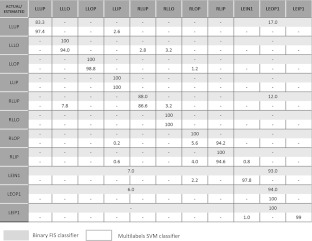
The main results from the previous multilabels SVM classifier for lung and lesion regions resulted in average sensitivity of 89.04 % obtained by averaging over the single sensitivities obtained in the recognition of the 12 tissue classes described above. In the present approach, we have implemented a binary classification by combining redundant lesion classes into one class C₂ and healthy lung tissues in class C₁. The sensitivity of fuzzy classifier is 96 % for lesion and 99 % for healthy tissues. The false-positive rate is 3 % as compared to our previous approach of 14.8 %. In order to provide a more accurate comparison with the previous multilabels approach, in Table 4 we summarize the distribution of the false positives assignments in terms of the 11 tissue classes (class BACK has been initially removed as already outlined) and we also report the results obtained in [18] in terms of average detection rate.

Table 4.

A comparison of the results obtained using the multilabels SVM classifier (light rectangles) and the binary FIS classifier (dark rectangles)

The results obtained by the described FIS binary classifier are also graphically reported in terms of ROC in Fig. 6: the dark curve is related to the lesion and the light curve to the healthy tissue. We obtain AUC = 0.98 for the lesions and AUC = 0.93 for the healthy tissue. The markers locate the two optimal operating points automatically extracted by the program and corresponding to sensitivity = 0.96 and specificity = 0.98 for the lesions, sensitivity = 0.99 and specificity = 0.94 for the healthy tissue. Table 5 also reports for each class the number of correctly classified and misclassified cases in the given test set. Finally, Table 6 reports the false-negative rate (FNR), the FPR, and the TPR for each class.

Fig. 6.

The ROC curves for the FIS. The dark curve is related to lesions and the light curve to the healthy tissue. The markers locate the optimal operating points automatically identified for the two curves

Table 5.

Confusion matrix of the classification result

	Actual C1	Actual C2
Assigned C1	44	2
Assigned C2	3	89

Table 6.

Performance metrics for classification using FIS

	FNR	FPR	TPR
C1	0.0638	0.0426	0.9362
C2	0.0220	0.0330	0.9780

From Table 4, we can observe that the FPs for the healthy tissue are mostly located in classes LLUP and RLUP. Conversely, the errors related to the misclassification of lesion tissue appear in classes LEIN1 and LEOP1. Further studies on the introduction of additional parameters could reduce the global error rate.

Discussion

Let us provide a critical review of the proposed method and future directions for the research in this context.

Advantages

One of the most appealing aspect of the proposed FIS is related to the fact that the radiologist can easily interfere with the system according to his/her experience. For example, physicians can add linguistic rules to the rules set, either suggesting new features to evaluate or manually changing the incidence level of a feature in order to emphasize a rule with respect to the others. So, the CAD can learn from expert radiologists in a very direct and easy way. The same possibility cannot be obtained using black box approaches such as neural networks or LDA classifiers, despite their classification capability.

Secondly, the output membership degrees assigned by the FIS to the considered portion or region of interest are not complementary and depend on both the incidence levels of the used features and on the features distribution on the training population. This issue can be important in order to guide a failure analysis that is the analysis of the circumstances under which an algorithm fails and the correction of the failure causes. In particular, when both the membership degrees are very low with respect to those assigned to other images, this fact can be related to the image itself, to the features evaluated on that image, to the characteristics of the training population, or finally to the selection of the algorithm parameters. This approach can be a guide to identify the most critical cases or to look for an algorithm improvement.

Regarding a comparative analysis, we have conducted experiments with the same dataset by using a simple SVM as described in [18]. Although the study was done by using a multilabels classification, implemented using a one versus all (1vsall) approach and random sampling methods for balancing the dataset, it was found that classifier gave high false alarm. One of the reasons for SVM classifier to perform not so good on this dataset can be that it considers all training samples uniformly and is sensitive to outliers and noise. However, fuzzy classifier (as proposed above) assigns different degrees of membership to samples thus reducing the effect of outliers and noise. This is particularly true in our case as the tissues pertaining to lung and lesion as delineated from HRCT scans and can be very prone to noise and outliers. In conclusion, the fuzzy classifier is seen to outperform the previous attempts of classifying this dataset at the cost of reducing the multiclass problem to a two-class problem.

Main Limitations

The limitation of this procedure is that it reduces the classification process from multilabels to binary. This methodology implies that information related to the tracking of different healthy tissues is not available. Thus, we can use the classifier for optimal treatment planning of the tumor but cannot take healthy tissue into consideration.

Future Directions

The present approach with a robust and easy way to interpret classifier opens the possibility of automatically tracking tumor motion in a 4DCT sequence without the need for clinician to repeatedly redefine the tumor position/contour. In the future, we will run the classifier on a 4DCT sequence for obtaining accurate and updated 3D tumor trajectory of the tumor at the time of radiation delivery. In addition, we will extend the classifier to multiclasses for healthy tissue recognition so that optimal treatment planning can be made, by taking into consideration the location of healthy lung tissues at the time of radiation delivery.

Additional features describing the orientation of the lung portions will be investigated in order to improve the capability of the classifier to distinguish classes 3 and 7, 4 and 8, 1 and 5, and 2 and 6 for healthy tissue.

References

- 1.Xing L, Siebers J, Keall P. Computational challenges for image-guided radiation therapy: framework and current research. Semin Radiat Oncol. 2007;17(4):245–257. doi: 10.1016/j.semradonc.2007.07.004. [DOI] [PubMed] [Google Scholar]
- 2.Keall PJ, et al. Four-dimensional radiotherapy planning for DMLC-based respiratory motion tracking. Med Phys. 2005;32(4):942–951. doi: 10.1118/1.1879152. [DOI] [PubMed] [Google Scholar]
- 3.Padley SPG, Hansell DM, Flower CDR, Jennings P. Comparative accuracy of high resolution computed tomography and chest radiography in the diagnosis of chronic diffuse infiltrative lung disease. Clin Radiol. 1991;44(4):222–226. doi: 10.1016/S0009-9260(05)80183-7. [DOI] [PubMed] [Google Scholar]
- 4.Urie MM, Goiten M, Doppke K, Kutcher JG, LoSasso T, Mohan R, Munzenrider JE, Sontag M, Wong JW. The role of uncertainity analysis in treatment planning. Int J Radiat Oncol Biol Phys. 1991;21:91–107. doi: 10.1016/0360-3016(91)90170-9. [DOI] [PubMed] [Google Scholar]
- 5.Ekberg L, Holmberg O, Wittgren L, Bjelkengren G, Landberg T. What margins should be added to the clinical target volume in radiotherapy treatment planning for lung cancer? Radiother Oncol. 1998;48:71–77. doi: 10.1016/S0167-8140(98)00046-2. [DOI] [PubMed] [Google Scholar]
- 6.Graham MV, Matthews JW, Harms WB, Sr, Enami B, Glazer HS, Purdy JA. Three dimensional radiation treatment planning study for patients with carcinoma of the lung. Int J Radiat Oncol Biol Phys. 1994;29:1105–1117. doi: 10.1016/0360-3016(94)90407-3. [DOI] [PubMed] [Google Scholar]
- 7.Leunens G, Menten J, Weltens C, Verstraete J, Van der Schueren E. Quality assessment of medical decision making in radiation oncology: variability in target volume delineation for brain tumors. Radiother Oncol. 1997;29:169–175. doi: 10.1016/0167-8140(93)90243-2. [DOI] [PubMed] [Google Scholar]
- 8.Tait D, Nahum A. Conformal therapy. Eur J Cancer. 1990;26:750–753. doi: 10.1016/0277-5379(90)90135-G. [DOI] [PubMed] [Google Scholar]
- 9.Hamilton CS, Denham JW, Joseph DJ, Labm DS, Spry NA, Gray AJ, Atkinson CH, Wynne CJ, Abdelaal A, Bydder PV, Chapman PJ, Matthews JHL, Stevens G, Ball D, Kearsley J, Ashcroft JB, Janke P, Gutmann A. Treatment and planning decisions in non-small cell carcinoma of the lung: an Australasian patterns of practice study. Clin Oncol R Coll Radiol. 1992;4:141–147. doi: 10.1016/S0936-6555(05)81075-1. [DOI] [PubMed] [Google Scholar]
- 10.Dewas S, Bibault J-E, Blanchard P, Vautravers-Dewas C, Pointreau Y, Denis F, Brauner M, Giraud P. Delineation in thoracic oncology: a perspective study of the effect of training on contour variability and dosimetric consequences. Radiat Oncol. 2011;6:118–127. doi: 10.1186/1748-717X-6-118. [DOI] [PMC free article] [PubMed] [Google Scholar]
- 11.Vorwerk H, Beckmann G, Bremer M, Degen M, Dietl B, et al. The delineation of target volumes for radiotherapy of lung cancer patients. Radiother Oncol. 2009;91:455–460. doi: 10.1016/j.radonc.2009.03.014. [DOI] [PubMed] [Google Scholar]
- 12.Giraud P, Elles S, Helfre S, Rycke YD, Servois V, et al. Conformal radiotherapy for lung cancer: different delineation of the gross tumor volume (GTV) by radiologists and radiation oncologists. Radiother Oncol. 2002;62:27–36. doi: 10.1016/S0167-8140(01)00444-3. [DOI] [PubMed] [Google Scholar]
- 13.Wiemker R., Rogalla P., Zwatkruis A., and Blaffert T., “Computer aided lung nodule detection on high resolution CT data,” Spie Med. Imag., pp. 677-688, 2002
- 14.Armato SG, Giger ML, Moran CJ, Blackburn JT, Doi K, MacMahon H. Computerized detection of pulmonary nodules on CT scans. RadioGraphics. 1999;19:1303–1311. doi: 10.1148/radiographics.19.5.g99se181303. [DOI] [PubMed] [Google Scholar]
- 15.Armato SG, Altman MB, Wilkie J, Sone S, Li F, Doi K, Roy AS. Automated lung nodule classification following automated nodule detection on CT: A serial approach. Med Phys. 2003;19:1188–1197. doi: 10.1118/1.1573210. [DOI] [PubMed] [Google Scholar]
- 16.Li Q. Recent progress in computer aided diagnosis of lung nodule on this section CT. Comp Med Imag Graph. 2007;4–5:248–257. doi: 10.1016/j.compmedimag.2007.02.005. [DOI] [PMC free article] [PubMed] [Google Scholar]
- 17.Goo JM. A computer aided diagnosis for evaluating lung nodules on chest CT: the current status and perspective. Korean J Radiol. 2011;12(2):145–155. doi: 10.3348/kjr.2011.12.2.145. [DOI] [PMC free article] [PubMed] [Google Scholar]
- 18.Kakar M, Olsen DR. Automatic segmentation and recognition of lungs and lesion from CT scans of thorax. Comput Med Imag Graph. 2009;33(1):72–82. doi: 10.1016/j.compmedimag.2008.10.009. [DOI] [PubMed] [Google Scholar]
- 19.Seiler PG, Blattmann H, Kirsch S, Muench RK, Schilling C. A novel tracking technique for the continuous precise measurement of tumor positions in conformal radiotherapy. Phys Med Biol. 2000;45:103–110. doi: 10.1088/0031-9155/45/9/402. [DOI] [PubMed] [Google Scholar]
- 20.Sharp GC, Jiang SB, Shimizu S, Shirato H. Tracking errors in a prototype real time tumour tracking system. Phys Med Biol. 2004;49:5347–5356. doi: 10.1088/0031-9155/49/23/011. [DOI] [PubMed] [Google Scholar]
- 21.Arslan S, Yilmaz A, Bayramgurler B, Uzman O, Nver E, Akkaya E. CT-guided transthoracic fine needle aspiration of pulmonary lesions: accuracy and complications in 294 patients. Med Sci Monit. 2002;8:493–497. [PubMed] [Google Scholar]
- 22.Geraghty PR, Kee ST, McFarlane G, Razavi MK, Sze DY, Dake MD. CT guided transthoracic needle aspiration biopsy of pulmonary nodules: needle size and pneumothorax rate. Radiology. 2003;229:475–481. doi: 10.1148/radiol.2291020499. [DOI] [PubMed] [Google Scholar]
- 23.Hosaik JD, Sixel KE, Tirona R, Cheung PC, Pignol JP. Correlation of lung tumor motion with external surrogate indicators of respiration. Int J Radiat Oncol Biol Phys. 2004;60:1298–1306. doi: 10.1016/j.ijrobp.2004.07.681. [DOI] [PubMed] [Google Scholar]
- 24.Berbeco RI, Nishioka S, Shirato H, Chen GT, Jiang SB. Residual motion of lung tumors in gated radiotherapy with external respiratory surrogates. Phys Med Biol. 2005;50:3655–3667. doi: 10.1088/0031-9155/50/16/001. [DOI] [PubMed] [Google Scholar]
- 25.Watanabe H, et al. The application of a fuzzy discriminant analysis for the diagnosis of valvular heart disease. IEEE Trans on Fuzzy Syst. 1994;2(4):267–276. doi: 10.1109/91.324806. [DOI] [Google Scholar]
- 26.Stevens CW, Munden RF, Forster KM, Kelly JF, Liao Z, Starkschall G, Tucker S, Komaki R. Respiratory-driven lung tumor motion is independent of tumor size, tumor location, and pulmonary function. Int J Radiat Oncol Biol Phys. 2001;51:62–68. doi: 10.1016/S0360-3016(01)01621-2. [DOI] [PubMed] [Google Scholar]
- 27.Colgan R, McClelland RJ, McQuaid D, Evans PM, Hawkes D, Brock J, Landau D, Webb S. Planning lung radiotherapy using 4d CT data and a motion model. Phys Med Biol. 2008;53:5815–5832. doi: 10.1088/0031-9155/53/20/017. [DOI] [PubMed] [Google Scholar]
- 28.M. Kakar and D.R. Olsen. Hybrid intelligent modeling and prediction of texture segmented lesion from 4DCT scans of thorax. In IEEE Conf. on Fuzzy Systems, Jeju, Korea, 2009
- 29.Zadeh LA. Fuzzy Sets Inf Control. 1965;8:338–353. doi: 10.1016/S0019-9958(65)90241-X. [DOI] [Google Scholar]
- 30.Andersson ER. Fuzzy and rough techniques in medical diagnosis and medication. Studies in fuzziness and soft computing. Heidelberg: Springer; 2007. [Google Scholar]
- 31.Mencattini A, Salmeri M: Breast masses detection using phase portrait analysis and fuzzy inference systems. Int J Comput Assist Radiol Surg, 2011. doi:10.1007/s11548-011-0659-0 [DOI] [PubMed]
- 32.A. Ferrero et al. Uncertainty evaluation in a fuzzy classifier for microcalcifications in digital mammography. In IEEE Instrumentation and Measurement Technology Conference (IMTC ’10), Austin, TX, USA, May 2010
- 33.A. Mencattini et al. A study on a novel scoring system for the evaluation of expected mortality in ICU-patients. In IEEE International Workshop on Medical Measurements and Applications (MEMEA ’11), Bari, Italy, May 2011
- 34.Chawla NV, Boywer KW, Hall LO, Kegelmeyer WP., “SMOTE: synthetic minority over-sampling technique,” J Artif Intell Res, vol. 321, Jun, 2002