Segmentation and Visualization of a Large, High-Resolution Micro-CT Data of Mice

Abstract

High-resolution large datasets were acquired to improve the understanding of murine bone physiology. The purpose of this work is to present the challenges and solutions in segmenting and visualizing bone in such large datasets acquired using micro-CT scan of mice. The analyzed dataset is more than 50 GB in size with more than 6,000 2,048 × 2,048 slices. The study was performed to automatically measure the bone mineral density (BMD) of the entire skeleton. A global Renyi entropy (GREP) method was initially used for bone segmentation. This method consistently oversegmented skeletal region. A new method called adaptive local Renyi entropy (ALREP) is proposed to improve the segmentation results. To study the efficacy of the ALREP, manual segmentation was performed. Finally, a specialized high-end remote visualization system along with the software, VirtualGL, was used to perform remote rendering of this large dataset. It was determined that GREP overestimated the bone cross-section by around 30 % compared with ALREP. The manual segmentation process took 6,300 min for 6,300 slices while ALREP took only 150 min for segmentation. Automatic image processing with ALREP method may facilitate BMD measurement of the entire skeleton in a significantly reduced time, compared with manual process.

Electronic supplementary material

The online version of this article (doi:10.1007/s10278-012-9498-y) contains supplementary material, which is available to authorized users.

Background

Microcomputed tomography (micro-CT) has been an useful tool in imaging small objects under high resolution as early as 1989 [1]. The quality and use of micro-CT has grown considerably during the last 20 years due to several factors. The most important explanation for the increased use of micro-CT is the ability to construct an instrument from readily available parts [2,3] and the ability to reconstruct 3D using simple yet powerful algorithms, such as the Feldkamp algorithm [4]. Over the years, micro-CT has been used to study bone loss in mice from harvested small samples of bone [5–7]. The imaging setup for dissected bone is similar to that employed for full animal imaging. However, certain precautions need to be considered [8] in imaging a whole animal. The X-ray dose to the live animal has to be increased in order to maintain low noise and good resolution. The increased dose might pose significant risk to the well being of the animal. Despite these constraints, full animal imaging has been successfully been conducted [9,10]. Granton et al. [11] have demonstrated rapid imaging of rats using cone-beam micro-CT to noninvasively measure whole-body adipose tissue volume, lean tissue volume, skeletal tissue volume, and bone mineral content. Although the whole body was imaged, the volume size was 486 × 160 × 880, which is smaller than our dataset 2,048 × 2,048 × 6,300, a two orders of magnitude difference. Such large datasets present unique problems in computation and visualization.

We here describe the challenges to analyzing large datasets and present the corresponding solutions. We describe an automatic method for segmenting the bone and compare its results against manual segmentation. This study was conducted to analyze BMD. This analysis is commonly used to diagnose osteoporosis and estimate fracture risk. Using a noninvasive technique (i.e., micro-CT), one can observe bone-remodeling changes of the entire skeleton in a real-time longitudinal fashion.

The methods described in this paper will be used for quantifying the BMD at each slice. High-end visualization on the other hand can be used to visualize and query the distribution of BMD across various slices in 3D. It is also useful in visualizing the mice bone anatomy. Thus, visualization plays an important role in large datasets in order to understand the segmentation results.

Although the results presented here are for imaging of a dead mouse, protocols are being developed for in-vivo imaging live animals.

Methods

Micro-CT Imaging

Three healthy BALB/C mice of approximately 15 weeks in age were imaged using a Siemens Inveon micro-PET-CT system (Siemens AG, Munich, Germany). The mice were killed by asphyxiation with CO₂ and placed in a 4 °C refrigerator for 4–30 h (Fig. 7). Each mouse was removed from the refrigerator and affixed to a thin, concave, carbonate plank in a prone position. The cranial limbs were stretched superiorly, while caudal limbs were stretched inferiorly. Effort was placed to ensure that the spine was centered on the jig in a median plane. This construct was inserted into the micro-CT loading bay. Scout views were taken to verify correct position, distance and selection of the scan.

Fig. 7.

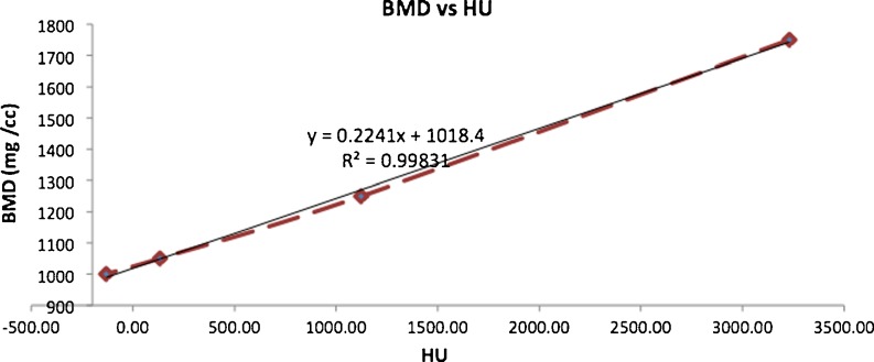
Calibration curve for BMD. The HU of a phantom containing inserts for which the value of electron density known was imaged and the curve was plotted. A straight line fit was then performed on the data points. The fitted line equation and the regression coefficient are shown

An X-ray technique of 80 kVp energy, 500 μA current, and an exposure time of 750 ms were used to image each mouse. The micro-CT scanner was set to a high magnification with a source to axis distance of 100 mm, the source to detector distance of 333.75 mm, and a cone angle of 21.15°. The reconstructed image slices were 2,048 × 2,048 pixels (37.66 × 37.66 mm) in the trans-axial dimension. The dataset composed of more than 6,000 axial slices with a total length of 113 mm. An Al filter (0.5 mm thickness) was selected in order to remove low energy photons and harden the beam. Four different couch positions were used to scan the entire 20-g carcass at high magnification with a pixel size of 18.38 μm and a binning factor of 2. At a projection angular interval of 2°, four rotations produced 720 projection images. Axial overlap of 20 % was stitched together for each rotation in order to reconstruct an image.

The Hounsfield unit (HU) was calibrated using 50 mL centrifuge tube filled with deionized water, using the same scanning setting used to scan the mouse. The Hounsfield unit was calculated using equation

where μ is the attenuation coefficient.

For calibrating BMD, a Siemens density phantom was scanned with same protocol as the mouse scan. The calibration phantom contained 4 bars of known densities: 1,750, 1,250, 1,050, and 1,000 mg/cc. The image of the bars were reconstructed and calibrated to HU. The resulting HU values for each bar were then used to determine the HU-to-BMD conversion formula (Fig. 7).

Segmentation

The first step in determining BMD is to segment the bone in the mouse dataset (Fig. 1). Since there are large numbers of slices, The global Renyi entropy (GREP) method [12] was used for segmentation. The algorithm was implemented in Matlab R2011a from Mathworks Inc. In the GREP method, a single threshold was used to segment the entire slice. This single threshold for the entire image resulted in oversegmentation of the bone. Thus, gaps (regions corresponding to bone marrow) in the original image were either filled completely or partially (shown by arrow) in the segmented image (Fig. 2). It also resulted in the segmented bone appearing larger than the original object. In order to overcome this, the adaptive local Renyi entropy (ALREP) method was used.

Fig. 1.

The original data and the corresponding segmented results. Left Original image, Middle segmentation result from GREP, right segmentation result from ALREP. The difference in the results between GREP and ALREP are better visualized using the region-of-interest shown in Fig. 2

Fig. 2.

Comparison of a region-of-interest of the slice in Fig. 1. Left Original image, center GREP, right ALREP method. Note that the GREP method resulted in over-segmentation (shown by arrows), causing fine gaps (marrow) to be filled in comparison with the original image

For each image, this process required:

1. Performing GREP and determine the necessary threshold.

2. Divide the image into multiple blocks.

3. For each block, determine if there are significant number of block pixels that have values greater than the GREP.

4. For a block containing a significant number of pixels, performed ALREP based thresholding.

5. Assemble the individual blocks to obtain the complete segmented image.

6. Determine the BMD value for the segmented regions using the relationship established by the method described in the previous section.

An expert in mice bone anatomy performed manual segmentation. For each dataset, 60 slices (approximately 1 % of the slices) were considered. These slices were segmented by manual thresholding using Avizo (Visualization Sciences group, Burlington, MA, USA) [13]. The threshold was chosen, such that the bone region was completely segmented. The expert manually corrected the pixels that were not segmented. BMD of the segmented region was calculated using a Matlab program (Mathworks, Inc; Natick, MA, USA) program. This program identified only the regions corresponding to the bone in the original slice data using the bone location in the manually segmented images. The mean value of BMD in the bone region was then calculated.

A third method, [14] called Yen method, was chosen as another automatic method for segmentation. It was chosen in order to compare the segmentation by ALREP. The Yen method has the computational complexity similar to ALREP. The slices used for manual segmentation were segmented using ALREP, GREP, and Yen method. The number of segmented pixels in each of the slice for different method was noted. A two-sample t test (α = 0.10) was conducted to study the significant difference between the number of segmented pixels in ALREP, GREP, and Yen method in relation to manual segmentation for each slice. Thus, the method that is consistently “significantly not different” from manual method will provide the best segmentation result.

Visualization

Since the dataset was large, a typical desktop computer will not able to process the data for visualization. Hence, a specialized high-end analysis and visualization system was used. It is a HP ProLiant ML370 G6 server with eight cores of 2.66 GHz Xeon X5550 and 64 GB of RAM (Hewlett-Packard, Inc.; Palo Alto, CA, USA). This analysis also required a high-speed network connection (10 GB Ethernet) for efficient transfer and storage of large datasets. VirtualGL (Austin, TX, USA) [15] was used as the software of choice for remote visualization, the process of rendering on a server and sending rendered image to the client. It provides any OpenGL based remote display software the ability to run with full 3D hardware acceleration on the server. It allows graphics scene to be rendered on the server and the resulting rendered image transferred to the client. Since rendering is performed on the server, the client does not need large graphics capabilities. The server intelligently compresses the rendered image in order to provide good frame rate. Thus, it can scale frame rates well, even if the dataset is large or the visualization process is complex. Avizo was used for visualization. The entire dataset (approximately 50 GB in size) was read completely into memory in order to perform iso-surface rendering (Figs. 6 and 7).

Fig. 6.

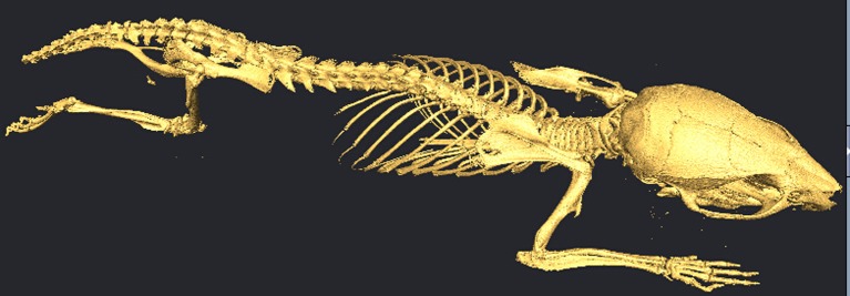
Iso-surface rendering of the mouse data using Avizo and VirtualGL

Two tests on the remote visualization system were conducted in order to determine its performance. The first test, nettest, was performed to determine the speed of the network between the client and the server. This test involves transferring datasets from 1 byte to 4 MB in multiples of 2 and measuring the throughput in Mbits per second. The second test was of frame rate. In this test, a standard dataset was volume rendered and the frame rate obtained by the client was measured. Remote visualization tools, like VirtualGL, drop rendered frames that a client does not have sufficient time to receive. This feature was disabled in order to measure the real frame rate.

Results

Segmentation

The left panel of Fig. 1 depicts the one slice of a mouse dataset. The image has been cropped and contrast enhanced to show only the region of data containing the mouse. The GREP method was first applied to the image; this is shown in the center panel of Fig. 1. The holes in the original image corresponding to marrow are either filled completely or partially. The bones at the bottom right and left corner of the image are larger than that in the original image. It is apparent then that the GREP method resulted in oversegmentation. This is better illustrated in the center panel in Fig. 2. This problem was resolved using ALREP. These results are shown in the right panel of Fig. 1 and the corresponding region of interest noted in the right panel of Fig. 2. The size of the segmented objects from ALREP more closely matches the original dataset. The significant differences in the number of segmented pixels will be discussed in the later part of this section.

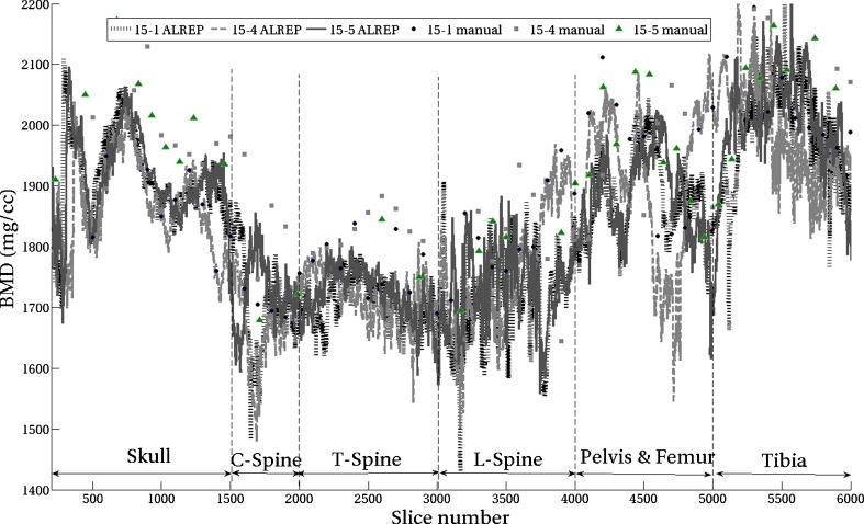
The average BMD value in the ALREP segmented bone region was determined and plotted for all slices shown in Fig. 3. This plot contains the results for all three imaged mice, titled 15-1, 15-4, and 15-5. The mean value of BMD for the manually segmented data for all three cases is also plotted in the same figure. The BMD based on ALREP method is plotted with lines, while the manually segmented values are plotted with markers at each data point. The x-axis is arranged so that the lower numbers are cranial while the higher numbers are at the tail of the mouse. The labels for various regions are also marked in Fig. 3. It can be seen that the three curves corresponding to the three mice follow similar patterns, but with different values for each slice.

Fig. 3.

Average value of bone mineral density in mg/cc from the segmented region determined using ALREP and the manual methods. ALREP results are labeled as 15-1 ALREP, 15-4 ALREP, and 15-5 ALREP; data points are connected by lines. The manual segmentation results are labeled as 15-1 manual, 15-4 manual, and 15-5 manual, and data points are shown by markers

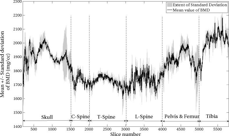
In order to visualize the variation in BMD for the same slice across three mice, a plot of means with standard deviations was created, as shown in Fig. 4. For a given slice (a vertical line in the plot), a point on the centerline is the average BMD value and the standard deviation of BMD flanks either side of the filled area. The lower numbers for the x-axis correspond to cranial region, while the higher numbers correspond to the tail of the mouse. The labels for various regions are also marked in the figure.

Fig. 4.

Average and standard deviation plot of BMD obtained using ALREP. The average with standard deviation is calculated across the three datasets. The centerline is the average BMD with standard deviation flanking either side

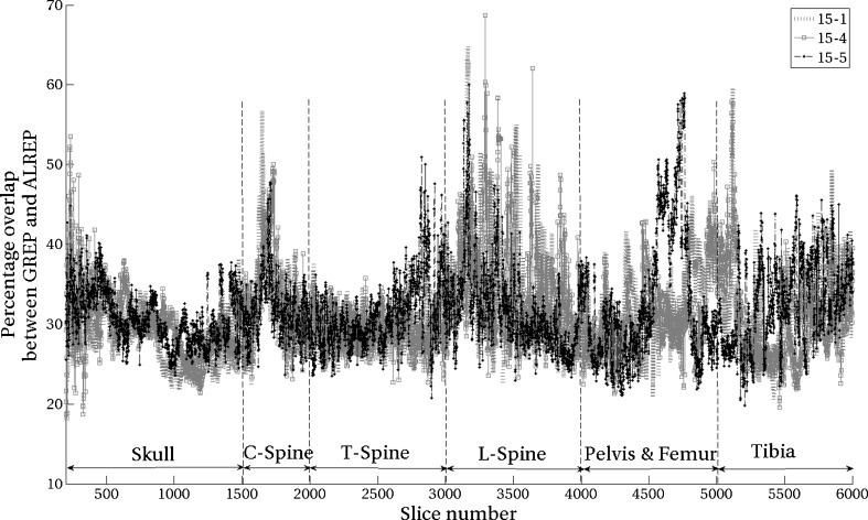
The number of pixels that are overestimated by GREP in comparison to ALREP are presented in Fig. 5. The mean value of the overestimation was 30 %. The overestimation is higher in the axial skeleton, where fine structures, such as trabeculae, are more common.

Fig. 5.

Oversegmentation by the GREP method compared to ALREP

The BMD calibration was performed based on the process described in “Micro-CT Imaging”; these results are presented in Fig. 7. The fitted curve has the following equation:

The regression coefficient of this relationship was r² = 0.998. The segmented pixel values (in HU) were processed using the above equation to obtain the corresponding BMD value.

The processing time for 6,300 slices was 150 min on a dual core 2.60 GHz processor with 4 GB of RAM. Although manual segmentation was performed for only 60 slices, it took 1 min to process one slice. Hence, for 6,300 slices, it would have consumed around 6,300 min or 4.4 days. Thus, the ALREP method has a processing time 40-fold faster when compared with manual segmentation and needs no manual intervention. Additionally, segmentation of this sizable dataset manually would potentially result in significant human error. Therefore, it is not a feasible long-term solution.

The method was tested against existing segmentation method like Yen method. The t test was conducted to study the significant difference between the number of segmented pixel in manual vs. each of the other methods, namely, GREP, ALREP, and Yen. ALREP did not have a significant difference from the manual method for all three mice. The GREP and Yen on the other hand have significant difference from the manual method for two out of three mice. Although the three methods have similar computational cost, ALREP provides a more consistent result with reference to manual segmentation and hence will be a choice for our future live animal imaging efforts.

Visualization

In the nettest, it was found that throughput was small, at around 1 Mbits/s for datasets of <1 MB. As the dataset becomes >1 MB, the throughput reaches ~1 Gbits/s, the speed of the network on the client side.

In the frame rate test, 27 frames per second were obtained for small datasets (2 MB), 10–12 frames per second for large datasets (50 GB with 2:1 binning), which are required for iso-surface rendering. The effective compressed data transfer rate was 13 Mbits/s between the server and the client.

Iso-surface visualization is shown in Fig. 6. The iso-surface contained around 20 million triangles. Rendering, along with the cross-section from the slices, was animated and demonstrated as a movie (Electronic Supplementary Material).

Discussion

A system for segmenting and visualizing large micro-CT dataset of mice was presented. The dataset is of size 2,048 × 2,048 × 6,300 pixels and around 50 GB in size. Since the dataset was large, it presents considerable challenge in automatic segmentation. The data was segmented to obtain the bone using GREP and ALREP. In the former, a single threshold limit was used to segment the image. GREP results in oversegmentation of the bone on an average by 30 % compared to ALREP. The addition of ALREP step did not increase the computational time significantly but improved the accuracy of segmentation considerably. Manual segmentation was performed to study the effectiveness of ALREP. The manual method of segmentation took 6,300 min (approximately) for 6,300 slices, while the automated method took only 150 min, 40 times faster than manual process. Since a typical desktop does not have the capability to read and render large datasets, a new high-end visualization system was used. VirtualGL and Avizo were used for visualization at 12 frames per second on a 1G bits/s network.

Step c in the ALREP method was used to determine whether a given block of the image has a significant number of pixels. The image was divided into 16 blocks along x-direction and 16 blocks along the y-direction. Each block thus has a size of 128 × 128 = 16,384 pixels. For analysis, a region was assumed as significant if it had at least 20 pixels with values greater than the global Renyi threshold. This 20-pixel value is significantly lower than the number of pixels in a block. Hence, increasing the number from 20 will not result in a substantial change in the block significance process.

The frame rate test throughput obtained only 13 Mbits/s, a very small number when compared to a network speed of 1 Gbit/s. The remote visualization involves the following steps: rendering 3D, compressing on the server, transferring rendered image over the network, decompressing on the client, and displaying. The nettest on the other hand involves only data transfer rate without computation. Since there are many processes required, the data generation rate is low; hence, the data transfer rate is also low. Even with 13 Mbits/s, 12 frames per second were achieved, thus providing close to a real-time frame rate. This enables VirtualGL to be used over slow network such as wireless and also from devices of different computational capabilities like laptops, tablets, phones, etc.

Translational Significance

This method can potentially be implemented to study the longitudinal effects of cancer treatment on entire skeleton thereby simulating recently developed preclinical [16] and clinical models [17] of cancer survivors’ bone health. Employing diagnostic CT using quantitative computed tomography in a clinical model, we have demonstrated that patients with ovarian or endometrial cancer experience an accelerated and distinct pattern of bone loss from systemic chemotherapy vs. local pelvic radiation. Many radiotherapy patients (example, head and neck or cervical cancers) undergo multiple whole-body PET-CT scans. These CT scans may be used to generate regional as well as complete skeletal BMD distribution, thereby providing important information on the heterogeneity of treatment effects following radiation, chemotherapeutic, or a combination of treatment modalities.

Conclusion

We have developed a method to automatically segment the bone and study its mineral density. We have demonstrated using a large dataset of size >50 GB that segmentation can be obtained within 150 min. This method has been shown to be considerably faster than manual segmentation. We also demonstrated the use of a specialized hardware and software for visualization of these datasets. In the future, this system will be used for in vivo study of changes in bone mineral density in a murine model to monitor treatment interventions.

The method has some limitations. The focus of the method was on segmenting the bone from the rest of the mouse. It does not segment other anatomical relevant regions such as organs, tissue, etc.

ALREP method has been demonstrated on sacrificed mice with parameters similar to live animal imaging. The future plan is to apply this method on live animal images and perform the longitudinal study of BMD. We are also interested in creating atlas of mice by defining regions such as skull, L-, C-, and T-vertebrae, tibia, femur, etc. The BMD will be studied in each of these regions. Subsequent mice data can be registered to this atlas and their BMD can be obtained automatically.

References

- 1.Feldkamp LA, et al. The direct examination of three-dimensional bone architecture in vitro by computed tomography. J Bone Miner Res. 1989;4:3–11. doi: 10.1002/jbmr.5650040103. [DOI] [PubMed] [Google Scholar]
- 2.Patel V, et al. Self-calibration of a cone-beam micro-CT system. Med Phys. 2009;36:48. doi: 10.1118/1.3026615. [DOI] [PMC free article] [PubMed] [Google Scholar]
- 3.Ionita CN, et al. Cone-beam micro-CT system based on LabVIEW software. J Digit Imaging. 2008;21(3):296–305. doi: 10.1007/s10278-007-9024-9. [DOI] [PMC free article] [PubMed] [Google Scholar]
- 4.Feldkamp LA, et al. Practical cone-beam algorithm. J Opt Soc Am. 1984;1:612–619. doi: 10.1364/JOSAA.1.000612. [DOI] [Google Scholar]
- 5.De Clerck NM, et al. Non-invasive high-resolution mCT of the inner structure of living animals. Microsc Anal. 2003;81:13–15. [Google Scholar]
- 6.Postnov AA, et al. 3D in vivo X-ray microtomography of living snails. J Microsc. 2002;205:201. doi: 10.1046/j.0022-2720.2001.00986.x. [DOI] [PubMed] [Google Scholar]
- 7.Postnov AA, et al. Quantitative analysis of bone mineral content by X-ray microtomography. Physiol Meas. 2003;24:165–167. doi: 10.1088/0967-3334/24/1/312. [DOI] [PubMed] [Google Scholar]
- 8.Holdsworth DW, et al. Micro-CT in small animal and specimen imaging. Trends Biotechnol. 2002;20(8):S34–S39. doi: 10.1016/S0167-7799(02)02004-8. [DOI] [Google Scholar]
- 9.Appleton CT et al: Forced mobilization accelerates pathogenesis: characterization of a preclinical surgical model of osteoarthritis. Arthritis Res Ther 9:R13, 2007 [DOI] [PMC free article] [PubMed]
- 10.McErlain DD, et al. Study of subchondral bone adaptations in a rodent surgical model of OA using in vivo micro-computed tomography. Osteoarthr Cartil. 2008;16:458–469. doi: 10.1016/j.joca.2007.08.006. [DOI] [PMC free article] [PubMed] [Google Scholar]
- 11.Granton PV, et al. Rapid in vivo whole-body composition of rats using cone-beam micro-CT. J Appl Physiol. 2010;109(4):1162–1169. doi: 10.1152/japplphysiol.00016.2010. [DOI] [PubMed] [Google Scholar]
- 12.Kapur JN, et al. A new method for gray-level picture thresholding using the entropy of the histogram. Graph Models Image Process. 1985;29(3):273–285. doi: 10.1016/0734-189X(85)90125-2. [DOI] [Google Scholar]
- 13.Avizo®. http://www.vsg3d.com/avizo/overview Accessed on 19 Aug 2011
- 14.Yen JC, Chang FJ, Chang S. A new criterion for automatic multilevel thresholding. IEEE Trans Image Process. 1995;4(3):370–378. doi: 10.1109/83.366472. [DOI] [PubMed] [Google Scholar]
- 15.The VirtualGL Project. http://www.virtualgl.org. Accessed on 19 Aug 2011
- 16.Hui SK, Fairchild GR, Kidder LS, Sharma M, Bhattacharya M, Jackson S, Le C, Yee D: Skeletal remodeling following clinically relevant radiation-induced bone damage treated with zoledronic acid. Calcif Tissue Int 90:40–49, 2012 [DOI] [PubMed]
- 17.Hui SK, Khalil A, Zhang Y, Coghill K, Le C, Dusenbery K, Froelich J, Yee D, Downs L. Longitudinal assessment of bone loss from diagnostic computed tomography scans in gynecologic cancer patients treated with chemotherapy and radiation. Am J Obstet Gynecol. 2010;203(4):353.e1–7. doi: 10.1016/j.ajog.2010.06.001. [DOI] [PMC free article] [PubMed] [Google Scholar]
Associated Data
This section collects any data citations, data availability statements, or supplementary materials included in this article.
Supplementary Materials