

Abstract
Traditional methods of exposure assessment in epidemiological studies often fail to integrate important information on activity patterns, which may lead to bias, loss of statistical power or both in health effects estimates. Novel sensing technologies integrated with mobile phones offer potential to reduce exposure measurement error. We sought to demonstrate the usability and relevance of the CalFit smartphone technology to track person-level time, geographic location, and physical activity patterns for improved air pollution exposure assessment. We deployed CalFit-equipped smartphones in a free living-population of 36 subjects in Barcelona, Spain. Information obtained on physical activity and geographic location was linked to space-time air pollution mapping. For instance, we found on average travel activities accounted for 6% of people’s time and 24% of their daily inhaled NO2. Due to the large number of mobile phone users, this technology potentially provides an unobtrusive means of collecting epidemiologic exposure data at low cost.
Keywords: smart phone, activity patterns, exposure, inhalation, air pollution, Global Positioning System
Introduction
Mobile phones are a ubiquitous technology throughout much of the developed and developing world. Many of these phones offer sensing capabilities that allow for tracking the movement patterns of their users through various environments, and thus potentially offer an innovative approach to enhance estimates of exposure to environmental hazards. The billions of current and future smart phone users worldwide (Pratt et al. 2012) afford an extraordinary opportunity for large scale data collection efforts that are cost-effective, accurate and unobtrusive.
Air pollution exposure assessment for use in epidemiological or health impact assessment studies has traditionally relied on fixed-site monitoring stations to assign ambient air pollution levels to large populations. More recently researchers have employed land use regression or dispersion models to estimate small-area concentrations at home addresses of study subjects. (Hoek et al. 2008; Jerrett et al. 2005) However, a person’s activities throughout the day may result in variability in exposures and inhalation of air pollution that may be substantial and unaccounted for when only home address-based concentrations are estimated.
Several studies comparing personal exposure measurements to ambient monitoring at subject’s home address have revealed at times large discrepancies between concentrations at residential addresses and personal exposure concentrations, and large variations from study-to-study and subject-to-subject. (Avery et al. 2010) Other studies indicated that activity patterns are important determinants of personal exposures (Schembari et al. In press; Valero et al. 2009). Recently, Dons et al. (2011) have shown that transport activities contribute most to variability in personal exposures between people exposed to the same concentrations at home. Further, estimating inhaled dose of air pollution by accounting for energy expenditure can change the relative ranking of exposures as a function of activity patterns compared to using solely exposure concentrations. (de Nazelle et al. 2012) Thus, exposure measurement errors introduced by failing to account for mobility and inhalation may lead to bias, loss of power, or both in health effects estimates. (Setton et al. 2011)
A growing body of research has used global positioning systems (GPS) to improve the measurement of a person’s location as it pertains to health. In environmental epidemiology (Elgethun et al. 2003; Phillips et al. 2001; Riediker et al. 2003) portable GPS technology improves the measurement of individuals’ exposures to hazards such as electromagnetic waves and pollution. Transportation researchers have used portable GPS technology to reconcile data on location, duration, and routes of individuals’ trips (Dill 2009; Duncan et al. 2009; Elgethun et al. 2007; Stopher et al. 2007) and, to evaluate the quality of data from self- reports. Physical activity researchers have used GPS to determine locations where physical activity occurs (Rodríguez et al. 2005; Troped et al. 2011; Wheeler et al. 2010), in an effort to identify which environments are conducive for physical activity and which environments pose barriers. Accelerometers are used in combinations with the GPS in these physical activity studies, but only as separate devices rather than in an integrated system. No previous studies have used GPS and motion-sensor technology in an integrated system such as a smartphone to simultaneously assess location and intensity of movements,
While the benefits of using GPS devices are increasingly recognized for exposure research, there are limitations to their widespread use, including the relatively high cost of equipment and time spent in field work to dispatch and collect data from subjects enrolled in personal measurement studies. A new opportunity emerges with the growing popularity of smartphones, which have integrated GPS systems and other sensor technology such as accelerometer, gyroscope, and magnetometer that are potentially useful for health-related research. The US National Academy of Sciences has recently called for the development of such novel ubiquitous and participatory sensing approaches to improve exposure science, in particular in integrated personalized monitoring and modeling frameworks (NAS 2012)
In this paper, we present results on the field use and performance of CalFit, a novel smartphone-based software that continuously records a subject’s time-location patterns and energy expenditure associated with physical activity using the phone’s integrated GPS and accelerometer, respectively, which we combined with spatial-temporal maps of air pollution. The main objective of this paper is to demonstrate the use of CalFit in tracking people’s movements in the urban environment and associated physical activity levels to improve air pollution exposure assessment.
Methods
Sample
A sample of 36 adults living and working in Barcelona was recruited for the study by way of emails sent to colleagues and friends of colleagues working at the CREAL research institute in Barcelona, Spain. The study took place from November 2010 to February 2011. Inclusion criteria were to live and work or study in Barcelona, live at more than a 10-minute walk away from work or school, and be able to ride a bicycle for 20 minutes. The study was approved by the Hospital del Mar Research Institute ethics committee.
Instruments
CalFit was developed through collaboration with researchers in Computer Science and Environmental Health Sciences at UC Berkeley. It consists of software that runs continuously in the background on an Android smartphone. CalFit records the phone’s triaxial accelerometry at 10 hertz (Hz), and a network-assisted global positioning system (aGPS) at 1 Hz. The CalFit application includes an algorithm that processes the accelerometry to estimate energy expenditure that adapts to the orientation of the phone, integrates motion in both vertical and horizontal directions, and uses the integrated vertical and horizontal accelerations (typically referred to as counts) within a generalized linear model to estimate energy expended within a sampling period (which for our study was 10 seconds). The aGPS improves the time-to-first-fix (TTFF) and can improve accuracy of the GPS, particularly in dense urban areas where GPS signals from satellites can often be obstructed. The algorithms (Gravina et al. 2010; Kuryloski et al. 2009; Seto et al. 2010; Yan et al. 2010) and their lab validation against the COSMED system are described elsewhere (Seto et al. 2011); as is the validation of the physical activity measurement in our current free-living population (Donaire-Gonzalez et al. submitted).
CalFit was installed on Google G1 Android phones retrofitted with larger size batteries to allow for a day of running CalFit. Phones were equipped with Subscriber Identity Module (SIM) cards with a data plan for phone and internet service from a local phone company, Yoigo.
Participant Procedures
Volunteers were scheduled to participate in the study during a week representative of their normal schedule. At the beginning of that week they met with a trained research assistant who provided them with details on the study protocol, obtained informed consent, and equipped them with the study instruments. The paper travel diary administered for this study was similar to most travel logs used in transportation studies, with entries for each trip on time of departure and arrival, purpose, travel mode(s), and destination address (see Supplemental material for additional information).
Data treatment and analysis
After downloading accelerometry and GPS files, we converted the energy intensity in Kcal (summed to a minute) to energy intensity in METs (metabolic equivalents; expressed as 1 kcal/kg/hour, approximately equivalent to the energy cost at rest) to have a same unit of measure on energy intensity independent of subjects’ weights and independent of activity duration for activity classification purposes.
When satellite signals were unavailable or too weak, CalFit provides location data from wireless network triangulation – a form of so-called Assisted GPS. These files gave less accurate geographic positions and were only used when satellite signals were not available.
Participants’ home and workplace address as well as any identifiable destination from the travel diary were geocoded using the City of Barcelona’s geocoding software (Instititut Municipal d’Informacio). The travel diary and CalFit data were merged to compare travel time periods logged in the diary to GPS tracking data, and to assign activity location and transport modes for each identified trip.
The GPS tracking data required post-processing. In particular, large clouds of data were formed when individuals were indoors. Also, when individuals traveled in narrow street canyons or in the metro observations sometimes dispersed or were missing. We used a point selection process with a manual check to clean up data for the selected day of each volunteer. Our process was to select in ArcGIS 9.3 (ESRI, Redlands, Ca) observations pertaining to clouds of data, assuming these to be associated with indoor activities, and then to check the time sequence of the selected points to detect probable departure from or arrival into the cloud. We confirmed the inferred indoor/outdoor and departure/arrival sequences based on records in the travel diary. We performed a final check examining the logic of time periods allocated to different activities. To focus our process we identified four such activity spaces: “home”, “work”, “other” indoor environments, and “in transit”, which included any movement outdoors (e.g., recreational outdoor activities).
We converted all observations to 1-minute averages of location and energy expenditure intensity in METs. To obtain a full data set we imputed for missing minutes geolocations and energy expenditure from previous and following observation in the same activity (only for two people for whom 11 and 13 minutes were missing, respectively). To best illustrate and to avoid bias from inferring missing data, and to avoid outlier activity, for each participant we selected the work day that offered the most complete data (in amount of recorded time).
Air pollution exposure
We overlaid street-scale maps of nitrogen dioxide (NO2) concentrations in Barcelona on our time-location data to estimate exposures or urban air pollution in our population sample. The NO2 annual mean map was obtained from an Atmospheric Dispersion Modeling System (ADMS)-Urban model developed for the year 2008 by Barcelona Regional for Barcelona’s Energy Agency, on a 5×5 m grid. (Barcelona Regional & Energy Agency of Barcelona 2011; Lao and Teixidó 2011) We developed the following adjustment factors to assign time-specific and microenvironment-specific concentration of each activity of each participant throughout the day, after inspecting hour and location of each activity from a combination of the GPS and diary data.
For the temporal adjustment we derived ratios, Ratioannual-t, between NO2 concentrations measured at a background monitoring station (MS) at time t (hour and day specific), CMS-t, compared to the annual mean concentration measured at the monitoring station, CMS-annual:.
We then applied these ratios to the annual mean NO2 prediction at point P from the dispersion model, CP-annual, to obtain the time-adjusted prediction at point P and time t, CP-t:
Additionally, we calculated adjustment factors for the hourly average concentration on workdays (i.e., for each hour of the day, the average concentration combining all workdays in a year) to provide more general profiles of exposures of our volunteers. Hourly measurements used in the analysis were provided by the Generalitat de Catulunya from the monitoring station “Vall d’Hebron”, the urban background monitoring station with most complete NO2 data for one year (August 2010 to July 2011).
Microenvironmental adjustments were derived from air pollution sampling campaigns conducted in Barcelona (See Table S1). In brief, indoor-outdoor ratios were obtained from simultaneous measurements of NO2 at subjects’ residence outside on a balcony or window sill and inside the home (Schembari et al. In press). We applied the same factor for all non-travel indoor environments (home, work, others). For the travel microenvironments we used available black carbon (BC) measurements as a proxy for NO2, assuming the behavior of these pollutants near traffic sources to be comparable (Beckerman et al. 2008). We considered that concentrations predicted by air pollution maps corresponded to concentrations experienced by pedestrians, and applied ratios obtained from BC measurements made during a 3-week monitoring campaign in Barcelona for the car, bike, bus and walk modes (de Nazelle et al. 2012). We assumed concentrations were the same in buses and trams, and we averaged the bike and car ratios for motorcycles. As we did not have any information for NO2 in metro or train systems, and did not find measurements of particulate matter of less than 2.5 micrometers in diameter (PM2.5)(Querol et al. 2012) to be an appropriate proxy for NO2 in the metro, we conservatively assumed levels to be equal to outside pedestrian-level exposures (Hong et al. 2005).
We assigned air pollution exposure to each participant in two ways: (1) concentration at the home address based on the annual mean of the map; and (2) time-weighted concentrations as a function of time-space activity. For the first approach, no adjustments were applied. For the second approach we compared exposure estimates obtained from (i) the annual mean of the map to those for which we integrated, (ii) the temporal adjustment, (iii) the microenvironmental adjustment, and (iv) both temporal and microenvironmental adjustment combined.
Finally we included inhalation rates derived from the physical activity measures to estimate inhaled air pollution as a function of activity patterns. Inhalation rates were calculated for each subject specific to their age, gender and weight, and energy expenditure level for each 1-minute observation using a series of stochastic equations described elsewhere (de Nazelle et al. 2009), and for which probability functions were set to their most likely value for the sake of illustration in this exercise. One-minute average inhalation rates were then multiplied by the corresponding exposure concentration to obtain the inhaled dose during that one-minute interval. We then estimated the contribution of various activity spaces (at home, work, in transit) to overall daily air pollution exposure and estimated daily inhalation of NO2. All analyses were conducted using R 2.14.1 (2011 The R Foundation for Statistical Computing).
Results
GPS and Compliance
All 36 volunteers who enrolled in the study completed the full protocol, except for one who did not complete the travel diary. Volunteers were mostly young (average age 31 years), well-educated (80% had university education) and two thirds female (see Table S2).
All participants had at least one day, and on average 4.2 days, of more than 10 hours of CalFit data registered during the day and evening (between 8 am and 10 pm, Table S3). Missing data were generally due to the loss of battery power, or failure to turn CalFit back on after cell phones shut down. On average less than 20% of daily waking hours were missing, and 75% of the participants had less than 0.5% of waking hours missing. At times during the day the CalFit system was turned on but participants were not wearing the cell phone (to charge the battery, because of aquatic activities, or in non-compliance with the protocol). Inspection of the CalFit physical activity data indicated that on average volunteers had a little over 3 days of at least 10 hours of data registered when the phone was actually worn. Almost half of the participants did not have a single day with 10 hours or more of GPS data recorded from satellite reception; on average only 1 day per participant had 10 or more hours of satellite data logged. As long as CalFit was working, some form of GPS data, whether from satellite signal or cell towers, was recorded, but the source was not necessarily identifiable due to lack of detailed files.
When selecting for each participant the work day with most data to perform the exposure analysis, we had to discard five participants due to insufficient data to non-compliance, illness, or technical problems. This left 31 individuals in the final analysis.
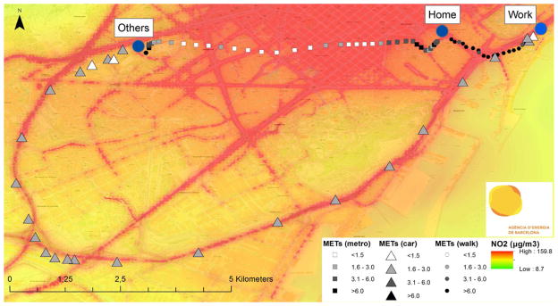
Figure 1 depicts all the activity from the 31 volunteers on their selected workday. On average for each day 22 hours of CalFit data, including 11 hours of Satellite GPS data, were recorded; the remaining hours were imputed to have full 24 hours of data for each participant.
Figure 1.

Selected 31 days of CalFit data (circles represent GPS tracking of participants, color intensity represent energy intensity); background shading is NO2 concentration.
Time-activity Profiles
Volunteers spent on average half of their time at home, where energy expenditure averaged 1 MET, a third at work (average energy expenditure 1.5 METs), and 6% traveling or in outdoor recreation (in movement) where the average energy expenditure reached 3.3 MET (Figure 3 (A) and see Table S4). The least variation in time spent in activity spaces between subjects was found for time spent at home (5 to 18 hours, or 23% to 76% of the day, with coefficient of variation (CV) = 0.19), and the greatest variation was found for times in other environments (13 volunteers only went to work and home on their work days, and others spent 20 minutes to 3 hours in “other” environments, CV=0.92). Volunteers spent from 30 minutes to close to 4 hours in transit on the selected day; the most common transportation modes in our sample were the bike, walk and metro.
Figure 3.

(A) Time spent in activity spaces; (B) NO2 concentration in activity spaces, derived from fully adjusted model (temporal and microenvironmental factors); (C) Percent contribution from different activity spaces to total time-weighted average NO2 concentration, using concentrations from fully adjusted model (temporal and microenvironmental factors); (D) Percent contribution to total NO2 daily inhaled dose from different activities, using concentrations from fully adjusted model (temporal and microenvironmental factors).
Exposure Assessment
Exposure concentrations were estimated for each participant according to the time, geoposition, and type of microenvironment of each activity throughout the day, as illustrated in Figure 2 for one participant. Concentrations in the various activity spaces (home, work, in transit and in other indoor environments) are shown for various adjustment methods in Table 1. When using solely the annual mean air pollution maps, we saw little variation between the average concentrations across individuals in the activity spaces (around 54 μg/m3 each), but at the individual level, concentrations at these locations could varied by as much as 40μg/m3. Once temporal adjustments were accounted for, contrasts between activity spaces were larger: in-transit time had the highest value on average, due to commute times occurring at time periods of highest concentrations. The microenvironmental adjustments led to higher exposure concentrations for travel activities compared to other activities. The combined temporal and microenvironmental adjustments therefore led to the greatest contrasts, with the highest exposures found in travel environments.
Figure 2.
Details of one day of activity for one participant.
Table 1.
NO2 (μg/m3) in different micro-environments according to different adjustment factors.
| Environments | Adjustment factors | mean ± SD | median (p25, p75) | CV | IQR | min | max |
|---|---|---|---|---|---|---|---|
| Home | annual mean map | 54 ± 11 | 52 (47, 61) | 0.2 | 14 | 38 | 76 |
| annual mean + temporal trend | 67 ± 26 | 57 (47, 89) | 0.39 | 43 | 28 | 114 | |
| annual mean + penetration | 55 ± 11 | 52 (48, 62) | 0.2 | 14 | 38 | 77 | |
| annual mean + penetration + temporal trend | 67 ± 26 | 57 (47, 90) | 0.39 | 44 | 28 | 115 | |
|
| |||||||
| Work | annual mean map | 53 ± 9 | 47 (47, 62) | 0.17 | 15 | 45 | 74 |
| annual mean + temporal trend | 61 ± 26 | 55 (42, 73) | 0.43 | 31 | 28 | 146 | |
| annual mean + penetration | 53 ± 9 | 47 (47, 63) | 0.17 | 16 | 45 | 75 | |
| annual mean + penetration + temporal trend | 62 ± 26 | 56 (43, 73) | 0.43 | 31 | 28 | 147 | |
|
| |||||||
| Other | annual mean map | 54 ± 16 | 50 (45, 60) | 0.29 | 16 | 35 | 93 |
| annual mean + temporal trend | 74 ± 50 | 65 (48, 81) | 0.67 | 33 | 23 | 254 | |
| annual mean + penetration | 55 ± 16 | 51 (45, 61) | 0.29 | 16 | 35 | 94 | |
| annual mean + penetration + temporal trend | 75 ± 50 | 66 (49, 82) | 0.67 | 33 | 23 | 256 | |
|
| |||||||
| In transit | annual mean map | 56 ± 5 | 56 (52, 60) | 0.09 | 9 | 45 | 66 |
| annual mean + temporal trend | 81 ± 25 | 75 (61, 93) | 0.31 | 32 | 44 | 132 | |
| annual mean + penetration | 81 ± 23 | 76 (60, 96) | 0.29 | 36 | 51 | 130 | |
| annual mean + penetration + temporal trend | 115 ± 49 | 94 (76, 158) | 0.42 | 82 | 56 | 228 | |
When we considered the impact of overall activity patterns on exposures by calculating time-weighted daily concentrations (Table 2), we found, compared to the traditionally used home address concentration, as much as a 15 μg/m3 difference in NO2 for an individual when using the annual mean map to estimate exposures. When additionally applying temporal and microenvironmental adjustment factors (full adjustment), we found as much as a 50μg/m3 difference in NO2 concentrations for an individual. On average, the difference between the fully adjusted NO2 exposure assignment and the home address concentration was 13μg/m3 (27% difference), with high variation across individuals (standard deviations 24 μg/m3, or 44%). The correlation between the “home address” and other methods was fairly high for the annual mean map method and also when microenvironmental adjustments were applied (Spearman coefficient = 0.81 (95% CI 0.6 to 0.9) and 0.78 (95% CI 0.6 to 0.9) respectively), but then dropped and became non-significant when comparing with the temporal adjustment method (Spearman coefficient = 0.09 (95% CI −0.2 to 0.4).
Table 2.
Exposure estimates for various exposures adjustment factors for NO2
| Home concentration (μg/m3) | Time weighted average concentration (μg/m3) with
|
||||
|---|---|---|---|---|---|
| annual mean map | temporal trend | penetration factor | penetration factor and temporal trend | ||
|
| |||||
| Mean | 54 | 54 | 64 | 56 | 67 |
| SD | 11 | 6 | 22 | 6 | 22 |
| Median | 52 | 53 | 63 | 55 | 64 |
| p.25% | 47 | 50 | 46 | 51 | 48 |
| p.75% | 61 | 58 | 80 | 60 | 83 |
| IQR | 14 | 8 | 34 | 8 | 35 |
| min | 38 | 42 | 30 | 42 | 31 |
| max | 76 | 68 | 108 | 70 | 112 |
| ICI | 50 | 51 | 57 | 53 | 59 |
| ICS | 58 | 56 | 72 | 58 | 75 |
|
| |||||
| Spearman coefficient a | - | 0.81 | 0.09 | 0.78 | 0.09 |
Spearman Correlation coefficient between the “Home address” method and the different time-weighted average methods.
Finally, when we integrated energy expenditure in the exposure calculations and estimated air pollution inhalation (Figure 3 (D) and see Table S5), we found that, on average, time at home, which represented 51% of people’s time in a day, and similarly 54% of daily time weighted exposures (Figure 3 (C) and see Table S6), accounted for only 40% of individuals’ total inhaled dose. Time at work, 33% of people’s daily activity, led to 29% daily time weighted exposures and 28% of daily inhaled NO2. In reverse, volunteers only spent 6% of their time in transit, yet this microenvironment contributed to 11% of time weighted exposures in a day, and 24% of daily inhaled NO2. Activities in “other” environments contributed least to time-weighted exposures (7%) and inhaled dose (8%) but had the most variable contributions across individuals (both percentages contribution CV = 1.4) and home activities contributed most and were the least variable (percent contribution CV = 0.2 and 0.3 respectively). Travel activities contributed over five times more to inhalation dose and more than four times more to daily exposures to NO2 per amount of time spent in the activity than any other activity.
Discussion
We conducted a study to demonstrate the use of CalFit for tracking personal movements in the urban environment and associated physical activity levels to improve air pollution exposure assessment. To illustrate the utility of the novel smart phone technology, the CalFit data were combined with modeled urban air pollution concentrations and data from the literature to estimate exposure and inhalation of urban air pollution accounting for the daily activities. We found that the smartphone system was feasible for our study of a free-living population and was efficiently integrated in a modeling framework to provide improvements in exposure assessment compared to traditional methods. To our knowledge, this is the first study to use smartphones as a means of improving air pollution exposure assessment. We obtained CalFit data for more than 10 waking hours a day (8am to 10pm) for on average four out of the five days of the study per participant. To illustrate the relevance of the CalFit system, we showed that compared to the traditionally used home-address method, accounting for time-activity patterns by assigning specific temporal and microenvironmental adjustment factors and accounting for time spent in each microenvironment substantially changes exposure concentrations: on average NO2 concentration assignments increased by 24% and variability between individuals as measured by the standard deviation doubled. We assessed the contribution of each activity space to overall exposure concentrations: on average in our population time spent at home contributed to 54% of daily time-weighted NO2 concentrations and time in transit 11%. A further benefit of CalFit is the measurement of physical activity that allows a calculation of inhaled dose of pollutants: for example, time at home on average accounted for 40% of intakes of NO2 and time in transit 24%. As a reference, these activities occupied respectively 53% and 6% of volunteers’ times on average.
Simulation studies have underscored the importance of travel activity as a source of daily air pollution exposures accounting for overall activity patterns (Gulliver and Briggs 2005). Dons et al. (2011) recently measured BC exposures with a portable microaethalometer while tracking movements with a GPS system in combination with an electronic diary in 16 individuals (8 couples). They concluded that travel activity contributes the most to variations in personal exposures between people.
Our approach provides an additional element in assessing exposures by allowing for estimates of intakes of air pollution, accounting for energy expenditures. We thus obtained an estimate closer to the actual internal dose to affect health than simply using exposure concentrations. In experimental and scripted settings, exercising while exposed to air pollutants has been shown to lead to intermediary health impacts (Mills et al. 2007; Weichenthal 2011). We did not, however, include breathing method (mouth or nose) in our calculation, nor did we attempt to estimate the uptake of pollutants, which may also vary according to activities (Daigle et al. 2003). The physical activity measurement error may also vary according to the activity type, leading to systematic errors in inhalation dose assessment as a function of activities. As with all accelerometers, certain activities such as cycling are indeed particularly difficult to assess (Butte et al. 2012). Using GPS in combination with accelerometers has been shown to improve classification of cycling activities (Troped et al). For future development of CalFit, an additional advantage over regular accelerometers is the potential to identify activities and match activity-specific energy expenditure algorithms, if these can be developed.
The advantages of the ubiquitous sensing approach are multiple. Most prominent of all is the sheer amount of potential data acquisition from billions of current and near-future smart phone users worldwide. We have shown that the approach is feasible and according to feedback from volunteers is of little intrusion to daily functioning. In comparison, traditional approaches used to assess activity patterns through activity or travel diaries are much more burdensome for study respondents, leading to under- or mis-reporting of travel activities. (Bricka and Bhat 2006) This was confirmed in our study, as most participants complained about the nuisance of filling out the travel log. Researchers have begun to use GPS systems as a promising alternative to such diaries. (Bricka et al. 2012; Rodríguez et al. 2005)
The CalFit smartphone system has several advantages over conventional GPS systems, including: the geopositioning information from mobile phone tower and Wi-Fi networks; the ability to access data directly from live-population without interference from a study protocol handling external devices; and the integration of different measurements (i.e. with a single time-stamp), such as physical activity, thus reducing lengthy merging post-processing of data. Other sensors could be integrated in the future, such as air pollution, noise, and UV radiation.
CalFit shares some of major challenges with GPS datalogging systems in general. One of the greatest hurdles encountered in this study was the post-processing of GPS data. There are advantages to acquiring geopositioning from cell phone towers from the internet provider when satellite reception fails: for example, places indoors or in narrow street canyons where satellite data is typically unavailable, some location information may still be gathered. The cell phone-tower positioning nevertheless tended to be highly inaccurate in our study, and thus added noise to the data, making trends more difficult to decipher. Few studies have taken on the task of interpreting activity patterns from continuous person-based GPS data (most travel or physical activity studies use data collected solely during the activity of interest and not continuously). Schuessler and Axhauseen (2009) used a series of cleaning, smoothing and rule-based algorithms and fuzzy logic to identify activities with mostly a focus on trip detection, including travel modes. Main inputs in the activity detection algorithm were speed, acceleration, dwell time, and point density. Unfortunately, while they were able to process a large amount of data efficiently (6.65 days of data for close to 5000 subjects), they had no data available (e.g. travel diary) to validate their approach. Wu et al. (2011) in contrast thoroughly checked travel logs, including follow-up calls, to establish a credible “gold standard” of activity patterns against which they compared to two GPS post-processing algorithms. Their models also used point density, speed and time sequencing as inputs, and performed well to identify indoor and in-vehicle activities, but not so well for outdoor static or walking activities. Hence even when simplifying activity patterns into only four categories and exploring various complex modeling approaches (rule based and random forest), still much work is needed to successfully identify activity patterns.
The integrated personalized monitoring and air pollution modeling framework, however, is limited by the quality and specificity of available air quality data. For instance, in our illustration temporal and microenvironmental adjustments are basic, using single microenvironmental ratio factors from ancillary studies or existing literature and a fixed monitoring station to scale hourly concentrations across the activity spaces. Such uncertainties can be reduced with improved spatial temporal mapping, or better characterized through MonteCarlo simulations for example (de Nazelle et al. 2009). Furthermore air pollution sensors could be connected to the smartphone to obtain measured data, without having to rely on modeled data.
The novelty of this paper is not in assessing time activity patterns, air pollution exposure and/or physical activity, which has been conducted and described before, but in the use of widely used smartphones in obtaining and integrating this information which enables the collection of such data in much larger populations on an individual level. This paper demonstrates a promising use of smartphones for exposure assessment, and highlights some further challenges with GPS data processing and automated activity recognition algorithms. Ubiquitous and participatory sensing technology provides new data collection opportunities to measure activity patterns, including levels of energy expenditure on a much wider scale than has been possible so far. Combined with air pollution modeling, or fairly soon measurements, it provides rich data that can reduce exposure measurement error and improve exposure estimates in epidemiological studies.
Supplementary Material
Higlhlights.
We track people’s movement and physical activity level using smart phone technology
We illustrate use of the technology to assess air pollution exposure and inhalation
Data from smart phones are integrated with air quality models
Smart phones will be connected to air pollution and other sensors in the future
Acknowledgments
We thank the Agència d’Energia de Barcelona and Barcelona Regional for the use of their NO2 dispersion model developed for Barcelona. Funding for this project was provided by the Centre for Research in Environmental Epidemiology (CREAL) Internal Grant Program, the Coca-Cola Foundation through the Transportation Air pollution and Physical ActivitieS (TAPAS) Program, and NIH NIEHS grant R01-ES020409. Finally, we thank Dr. Ruzena Bajcsy and seed funding from the Center for Information Technology in the Interest of Society (CITRIS), which were instrumental in the development of CalFit.
Footnotes
Methods details and description of the sample sociodemographic characteristics, CalFit records, activity patterns records, and NO2 exposure and inhalation, available online.
Publisher's Disclaimer: This is a PDF file of an unedited manuscript that has been accepted for publication. As a service to our customers we are providing this early version of the manuscript. The manuscript will undergo copyediting, typesetting, and review of the resulting proof before it is published in its final citable form. Please note that during the production process errors may be discovered which could affect the content, and all legal disclaimers that apply to the journal pertain.
References
- Avery CL, Mills KT, Williams R, McGraw KA, Poole C, Smith RL, et al. Estimating Error in Using Ambient PM2.5 Concentrations as Proxies for Personal Exposures: A Review. Epidemiology. 2010;21:215–223. doi: 10.1097/EDE.0b013e3181cb41f7. [DOI] [PMC free article] [PubMed] [Google Scholar]
- Barcelona Regional & Energy Agency of Barcelona. Barcelona city council. Barcelona city council; Barcelona: 2011. PECQ, Pla d’Energia, Canvi Climatic i Qualitat de l’Aire de Barcelona 2011–2020. [Google Scholar]
- Beckerman B, Jerrett M, Brook JR, Verma DK, Arain MA, Finkelstein MM. Correlation of nitrogen dioxide with other traffic pollutants near a major expressway. Atmos Environ. 2008;42:275–290. doi: 10.1016/j.atmosenv.2007.09.042. [DOI] [Google Scholar]
- Bricka S, Bhat C. Comparative Analysis of Global Positioning System-Based and Travel Survey-Based Data. Transport Res Rec. 2006;1972:9–20. doi: 10.3141/1972-04. [DOI] [Google Scholar]
- Bricka SG, Sen S, Paleti R, Bhat CR. An analysis of the factors influencing differences in survey-reported and GPS-recorded trips. Transport Res C-Emer. 2012;21:67–88. doi: 10.1016/j.trc.2011.09.005. [DOI] [Google Scholar]
- Butte NF, Ekelund U, Westerterp KR. Assessing physical activity using wearable monitors: measures of physical activity. Med Sci Sports Exerc. 2012;44:S5–12. doi: 10.1249/MSS.0b013e3182399c0e. [DOI] [PubMed] [Google Scholar]
- Committee on Human and Environmental Exposure Science in the 21st Century; Board on Environmental Studies and Toxicology; Division on Earth and Life Studies; National Research Council. Exposure Science in the 21st Century: A Vision and a Strategy. The National Academies Press; Washington, D.C: 2012. [PubMed] [Google Scholar]
- Daigle CC, Chalupa DC, Gibb FR, Morrow PE, Oberdörster G, Utell MJ, Frampton MW. Ultrafine particle deposition in humans during rest and exercise. Inhal Toxicol. 2003;15:539–552. doi: 10.1080/08958370304468. [DOI] [PubMed] [Google Scholar]
- de Nazelle A, Fruin S, Westerdahl D, Martinez D, Ripoll A, Kubesch N, et al. A travel mode comparison of commuters’ exposures to air pollutants in Barcelona. Atmos Environ. 2012;59:151–159. doi: 10.1016/j.atmosenv.2012.05.013. [DOI] [Google Scholar]
- de Nazelle A, Rodríguez DA, Crawford-Brown D. The built environment and health: Impacts of pedestrian-friendly designs on air pollution exposure. Sci Total Environ. 2009;407:2525–2535. doi: 10.1016/j.scitotenv.2009.01.006. [DOI] [PubMed] [Google Scholar]
- Dill J. Bicycling for Transportation and Health: The Role of Infrastructure. J Public Health Policy. 2009;30:S95–S110. doi: 10.1057/jphp.2008.56. [DOI] [PubMed] [Google Scholar]
- Donaire-Gonzalez D, de Nazelle A, Seto E, Mendez M, Nieuwenhuijsen M, Jerrett M. Comparison of physical activity measures using smartphone based CalFit and Actigraph. J Med Internet Res. doi: 10.2196/jmir.2470. Submitted. [DOI] [PMC free article] [PubMed] [Google Scholar]
- Dons E, Int Panis L, Van Poppel M, Theunis J, Willems H, Torfs R, et al. Impact of time-activity patterns on personal exposure to black carbon. Atmos Environ. 2011;45:3594–3602. [Google Scholar]
- Duncan MJ, Badland HM, Mummery WK. Applying GPS to enhance understanding of transport-related physical activity. J Sci Med Sport. 2009;12:549–556. doi: 10.1016/j.jsams.2008.10.010. [DOI] [PubMed] [Google Scholar]
- Elgethun K, Fenske RA, Yost MG, Palcisko GJ. Time-location analysis for exposure assessment studies of children using a novel global positioning system instrument. Environ Health Perspect. 2003;111:115–122. doi: 10.1289/ehp.5350. [DOI] [PMC free article] [PubMed] [Google Scholar]
- Elgethun K, Yost MG, Fitzpatrick CTE, Nyerges TL, Fenske RA. Comparison of global positioning system (GPS) tracking and parent-report diaries to characterize children’s time|[ndash]|location patterns. J Expo Sci Environ Epidemiol. 2007;17:196–206. doi: 10.1038/sj.jes.7500496. [DOI] [PubMed] [Google Scholar]
- Gravina R, Alessandro A, Salmeri A, Buondonno L, Raveendranathan N, Loseu V, et al. Enabling Multiple BSN Applications Using the SPINE Framework. Proceedings of the 2010 International Conference on Body Sensor Networks. 2010:228–233. doi: 10.1109/BSN.2010.34. [DOI] [Google Scholar]
- Gulliver J, Briggs DJ. Time-space modeling of journey-time exposure to traffic-related air pollution using GIS. Environ Res. 2005;97:10–25. doi: 10.1016/j.envres.2004.05.002. [DOI] [PubMed] [Google Scholar]
- Hoek G, Beelen R, De Hoogh K, Vienneau D, Gulliver J, Fischer P, et al. A review of land-use regression models to assess spatial variation of outdoor air pollution. Atmos Environ. 2008;42:7561–7578. doi: 10.1016/j.atmosenv.2008.05.057. [DOI] [Google Scholar]
- Hong Y-C, Leem J-H, Lee K-H, Park D-H, Jang J-Y, Kim S-T, et al. Exposure to air pollution and pulmonary function in university students. Int Arch Occup Environ Health. 2005;78:132–138. doi: 10.1007/s00420-004-0554-x. [DOI] [PubMed] [Google Scholar]
- Jerrett M, Arain A, Kanaroglou P, Beckerman B, Potoglou D, Sahsuvaroglu T, et al. A review and evaluation of intraurban air pollution exposure models. J Expo Anal Environ Epidemiol. 2005;15:185–204. doi: 10.1038/sj.jea.7500388. [DOI] [PubMed] [Google Scholar]
- Kuryloski P, Giani A, Giannantonio R, Gilani K, Gravina R, Seppa V-P, et al. DexterNet: An Open Platform for Heterogeneous Body Sensor Networks and its Applications. Proceedings of the 2009 Sixth International Workshop on Wearable and Implantable Body Sensor Networks. 2009:92–97. doi: 10.1109/BSN.2009.31. [DOI] [Google Scholar]
- Lao J, Teixidó O. Air quality model for Barcelona. Air Pollution XIX. 2011:25–36. doi: 10.2495/AIR110031. [DOI] [Google Scholar]
- Mills NL, Törnqvist H, Gonzalez MC, Vink E, Robinson SD, Söderberg S, Boon NA, Donaldson K, Sandström T, Blomberg A, Newby DE. Ischemic and thrombotic effects of dilute diesel-exhaust inhalation in men with coronary heart disease. N Engl J Med. 2007;357:1075–1082. doi: 10.1056/NEJMoa066314. [DOI] [PubMed] [Google Scholar]
- Pratt M, Sarmiento OL, Montes F, Ogilvie D, Marcus BH, Perez LG, Brownson RC for the Lancet Physical Activity Series Working Group. The implications of megatrends in information and communication technology and transportation for changes in global physical activity. Lancet. 2012;380(9838):282–93. doi: 10.1016/S0140-6736(12)60736-3. [DOI] [PMC free article] [PubMed] [Google Scholar]
- Phillips ML, Hall TA, Esmen NA, Lynch R, Johnson DL. Use of global positioning system technology to track subject’s location during environmental exposure sampling. J Expo Anal Environ Epidemiol. 2001;11:207–215. doi: 10.1038/sj.jea.7500161. [DOI] [PubMed] [Google Scholar]
- Querol X, Moreno T, Karanasiou A, Reche C, Alastuey A, Viana M, et al. Variability of levels and composition of PM10 and PM2.5 in the Barcelona metro system. Atmos Chem Phys Discuss. 2012;12:6655–6713. doi: 10.5194/acpd-12-6655-2012. [DOI] [Google Scholar]
- Riediker M, Williams R, Devlin R, Griggs T, Bromberg P. Exposure to Particulate Matter, Volatile Organic Compounds, and Other Air Pollutants Inside Patrol Cars. Environ Sci Technol. 2003;37:2084–2093. doi: 10.1021/es026264y. [DOI] [PubMed] [Google Scholar]
- Rodríguez DA, Brown AL, Troped PJ. Portable global positioning units to complement accelerometry-based physical activity monitors. Med Sci Sports Exerc. 2005;37:S572–581. doi: 10.1249/01.mss.0000185297.72328.ce. [DOI] [PubMed] [Google Scholar]
- Schembari A, Triguero-Mas M, de Nazelle A, Dadvand P, Vrijheid M, Cirach M, et al. Personal, indoor and outdoor Air pollution levels among pregnant Women. Atmospheric Environment. doi: 10.1016/j.atmosenv.2012.09.053. In press. [DOI] [Google Scholar]
- Schuessler N, Axhausen KW. Processing Raw Data from Global Positioning Systems Without Additional Information. Transport Res Rec. 2009;2105:28–36. doi: 10.3141/2105-04. [DOI] [Google Scholar]
- Seto E, Martin E, Yang A, Yan P, Gravina R, Lin I, et al. Opportunistic strategies for lightweight signal processing for body sensor networks. Proceedings of the 3rd International Conference on PErvasive Technologies Related to Assistive Environments. 2010;56:1–56:6. doi: 10.1145/1839294.1839361. [DOI] [Google Scholar]
- Seto E, Yan P, Kuryloski P, Bajcsy R, Abresch T, Henricson E, et al. Mobile Phones as Personal Environmental Sensing Platforms: Development of the CalFit System. The 23rd Annual Conference of the International Society of Environmental Epidemiology (ISEE); 2011. [DOI] [Google Scholar]
- Setton E, Marshall JD, Brauer M, Lundquist KR, Hystad P, Keller P, et al. The impact of daily mobility on exposure to traffic-related air pollution and health effect estimates. J Expo Sci Environ Epidemiol. 2011;21:42–48. doi: 10.1038/jes.2010.14. [DOI] [PubMed] [Google Scholar]
- Stopher P, FitzGerald C, Xu M. Assessing the accuracy of the Sydney Household Travel Survey with GPS. Transportation. 2007;34:723–741. doi: 10.1007/s11116-007-9126-8. [DOI] [Google Scholar]
- Troped PJ, Tamura K, Whitcomb HA, Laden F. Perceived built environment and physical activity in U.S. women by sprawl and region. Am J Prev Med. 2011;41:473–479. doi: 10.1016/j.amepre.2011.07.023. [DOI] [PMC free article] [PubMed] [Google Scholar]
- Troped PJ, Oliveira MS, Matthews CE, Cromley EK, Melly SJ, Craig BA. Prediction of activity mode with global positioning system and accelerometer data. Med Sci Sports Exerc. 2008;40:972–978. doi: 10.1249/MSS.0b013e318164c407. [DOI] [PubMed] [Google Scholar]
- Valero N, Aguilera I, Llop S, Esplugues A, de Nazelle A, Ballester F, et al. Concentrations and determinants of outdoor, indoor and personal nitrogen dioxide in pregnant women from two Spanish birth cohorts. Environ Int. 2009;35:1196–1201. doi: 10.1016/j.envint.2009.08.002. [DOI] [PubMed] [Google Scholar]
- Weichenthal S, Kulka R, Dubeau A, Martin C, Wang D, Dales R. Traffic-related air pollution and acute changes in heart rate variability and respiratory function in urban cyclists. Environ Health Perspect. 2011;119:1373–1378. doi: 10.1289/ehp.1003321. [DOI] [PMC free article] [PubMed] [Google Scholar]
- Wheeler BW, Cooper AR, Page AS, Jago R. Greenspace and children’s physical activity: A GPS/GIS analysis of the PEACH project. Prev Med. 2010;51:148–152. doi: 10.1016/j.ypmed.2010.06.001. [DOI] [PubMed] [Google Scholar]
- Wu J, Jiang C, Houston D, Baker D, Delfino R. Automated time activity classification based on global positioning system (GPS) tracking data. Environ Health. 2011;10:101. doi: 10.1186/1476-069X-10-101. [DOI] [PMC free article] [PubMed] [Google Scholar]
- Yan P, Lin I, Roy M, Seto E, Wang C, Bajcsy R. WAVE and CalFit - Towards social interaction in mobile body sensor networks. Wireless Internet Conference (WICON), 2010 The 5th Annual ICST 1 –2.2010. [Google Scholar]
Associated Data
This section collects any data citations, data availability statements, or supplementary materials included in this article.