Choosing a design to fit the situation: how to improve specificity and positive predictive values using Bayesian lot quality assurance sampling

Abstract

Background Lot Quality Assurance Sampling (LQAS) is a provably useful tool for monitoring health programmes. Although LQAS ensures acceptable Producer and Consumer risks, the literature alleges that the method suffers from poor specificity and positive predictive values (PPVs). We suggest that poor LQAS performance is due, in part, to variation in the true underlying distribution. However, until now the role of the underlying distribution in expected performance has not been adequately examined.

Methods We present Bayesian-LQAS (B-LQAS), an approach to incorporating prior information into the choice of the LQAS sample size and decision rule, and explore its properties through a numerical study. Additionally, we analyse vaccination coverage data from UNICEF’s State of the World’s Children in 1968–1989 and 2008 to exemplify the performance of LQAS and B-LQAS.

Results Results of our numerical study show that the choice of LQAS sample size and decision rule is sensitive to the distribution of prior information, as well as to individual beliefs about the importance of correct classification. Application of the B-LQAS approach to the UNICEF data improves specificity and PPV in both time periods (1968–1989 and 2008) with minimal reductions in sensitivity and negative predictive value.

Conclusions LQAS is shown to be a robust tool that is not necessarily prone to poor specificity and PPV as previously alleged. In situations where prior or historical data are available, B-LQAS can lead to improvements in expected performance.

Introduction

Lot quality assurance sampling (LQAS) is a useful component of the health programme evaluation toolkit with an ever expanding range of applicability.¹ LQAS is a classification procedure designed for decision-making; for taking action.² The goal is to classify a partially measured group. For example, we might wish to classify the vaccination coverage in a given population (defined as the lot) as either acceptable or unacceptable, with respect to some desired programmatic threshold, p*.³ A traditional LQAS design comprises a sample size, n, and a decision rule, d, denoted (n, d). If in a random sample of n individuals the number of vaccinated individuals is greater than or equal to d, we classify the population as acceptable (p ≥ p* to place a number to our label). Otherwise, we classify it as unacceptable (p < p*).

The design parameters determine the statistical properties of the LQAS procedure. They are chosen to achieve pre-specified levels of misclassification risk at upper and lower thresholds, p_U and p_L, respectively. Namely, we choose the design so that the risk of incorrectly classifying a population as unacceptable when the coverage is at the upper threshold (p = p_U), or higher, is no greater than α (Producer risk), and the risk of incorrectly classifying a population as acceptable when the coverage is at the lower threshold (p = p_L), or lower, is no greater than β (Consumer risk). The programmatic threshold, p*, does not explicitly enter into the specification of the LQAS design, although ordinarily we implicitly assume that p_L ≤ p* ≤ p_U.

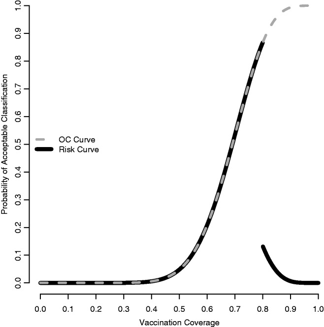
The two thresholds and their risks are a priori characteristics of the design. Traditionally, these characteristics are read from the Operating Characteristic (OC) curve, which plots the probability of classification as acceptable as a function of the underlying coverage. Figure 1 depicts the OC curve for an (18,13) design (with p_L = 0.50 and p_U = 0.80). It is clear, from the OC curve, that values of p lying between p_L and p_U, a region known as the ‘grey area’, are subject to relatively high risks of misclassification. Presumably, this region also represents that part of the parameter space where a misclassification error is of less consequence.

Figure 1.

Operating Characteristic (dashed grey) and Risk (solid black) Curves assuming p* = 0.80 for n = 18 and d = 13

The programmatic threshold plays an important rôle when evaluating the design attributes a posteriori. Sandiford in 1993 explored the a posteriori properties of LQAS using UNICEF measles vaccination data from 1968–1989 in 126 countries.^4,5 Ultimately, Sandiford asserted that LQAS ‘is a sensitive test for poor performance but in most settings probably not a particularly specific one’. This has unfortunately led to confusion in the literature, where in some cases researchers have inferred that LQAS in general is prone to poor specificity and, relatedly, to poor positive predicted value (PPV).^6–8 Sandiford’s findings were based on the assumed coverage distribution found in the UNICEF data and are not generalizable to ‘most settings’. This distribution is subject to change with time, for example, and to aptly assess the performance of the LQAS method we must consider other distributional contexts too.

Sandiford’s study raises the interesting question of how to address LQAS design in the presence of prior knowledge. When historical data are available, an intuitively appealing strategy is to choose a design that reduces the number of historical data points that lie in the grey region where the misclassification risk is high. Olives and Pagano formalize this notion using Bayesian-LQAS (B-LQAS), a Bayesian approach to choosing the decision rule when there is prior knowledge about the underlying coverage distribution.⁹ They use the decision rule for a fixed sample size that maximizes the figure of merit (FOM),

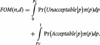where π(·) is the prior distribution of vaccination coverage. The FOM is thus the average, or expected, probability of correctly classifying coverage in the extremes, i.e. beyond the lower and upper thresholds. The resulting LQAS designs benefit from the optimality implied by the FOM and result in optimal classifications with respect to p* at the extremes.

The just-described approach ignores the grey area by putting zero weight there. In reality, even though the consequences of misclassification in this region may not be as serious as in the extremes, programme managers may feel that this region is important. Further, the original B-LQAS proposal did not include a provision for choosing the optimal sample size.

We now propose a generalization of B-LQAS that allows managers to incorporate the assumed programmatic threshold, p*, as well as p_L and p_U, and to weight various coverage regions differently, including the grey area, so as to choose both sample size and decision rule accordingly. We explore the properties of this generalized B-LQAS in a numerical study. Additionally, we revisit the Sandiford analysis to demonstrate how the performance of LQAS varies depending on the underlying distribution of vaccination coverage. To this end, we repeat Sandiford’s study but with more up-to-date measles vaccination data from UNICEF.¹⁰ We show that whereas the Consumer and Producer risks are preserved even with varying underlying distributions, other metrics such as sensitivity, specificity, PPV and negative predictive value (NPV) do change. Finally, we show that the use of generalized B-LQAS to choose sample sizes and decision rules improves the expected performance of classical LQAS for the UNICEF data.

Methods

Generalizing B-LQAS

Consider a new concept, the Risk Curve (RC), which displays the probability of an incorrect classification as a function of the true coverage:

The RC for LQAS design (18,13) is shown in Figure 1. The OC curve and RC convey similar information. However, the latter makes explicit the distinction between acceptable and unacceptable coverage with respect to p*, and also makes it easier to explain that ideally we wish to minimize the value of this function throughout its domain. With this notation in place, we propose a more general form of the FOM,

where w(·) is a non-negative weighting function that, over its range, reflects the relative importance of correct classification. The GFOM is a weighted average of correct classification and is closely related to the Bayes Risk in the decision-making literature.¹¹ Although we do not explore this connection further, we direct interested readers to.¹² Designs resulting from maximizing the GFOM benefit from the optimality implied by the GFOM and result in optimal classifications with respect to p* given the prior distribution and the chosen weighting function.

The weighting function w(·) reflects beliefs about the relative importance of classification for different coverages and incorporates information about the upper and lower thresholds. We consider the class of weight functions of the form

where p₁(p) and p₂(p) are known functions of the true coverage that do not depend on n or d, and w₁ and w₂ are weights for combining these two functions. A feature of this class of weighting functions is that the GFOM optimal decision rule relies on the relative value of the weights w₁ and w₂, but not on their absolute values (see Supplementary Appendix, available at IJE online).

A weighting function that simply contrasts the two extremes is,

a generalization of the FOM when w₁ = w₂ = 1. An alternative, and more appealing, set of weights,

makes explicit the role of p*, and the relative magnitude of w₁ to w₂ reflects the importance of classification below and above this target, respectively. Although w₂(·) is an improvement over w₁(·), it still gives all coverage above or below p* equal weight, whereas the consequence of misclassification might be related to the distance from p*. To incorporate these concerns, consider

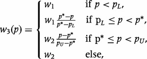where the importance of correct classification of the extremes is constant, but the importance of correctly classifying moderate coverage diminishes linearly as the prevalence approaches p*.

Selecting the sample size by B-LQAS

The above formulation is for fixed sample sizes. To additionally calculate the optimal sample size in the B-LQAS framework, consider the normalized weighting function, w*(·), where

Using w*(·) results in the same optimal decision rule for a given sample size [denoted d*(n)], and scales the GFOM to lie between zero and one, resulting in the more interpretable quantity, GFOM* (see Supplementary Appendix, available at IJE online). The optimal sample size can be chosen by finding the smallest n such that GFOM*(n, d*(n)) ≥ k, where k is the investigator-chosen minimum probability of correct classification. Here, we assume k = 0.95.

Numerical study of B-LQAS

To study the GFOM under varying assumptions about the underlying distribution of vaccination coverage, assume that the distribution of coverage follows a beta distribution with parameters s₁ and s₂. The beta family includes sufficiently varied shapes to provide a broad offering of prior distributions, and the integration in the GFOM can be solved analytically for each of the weighting functions considered (see Supplementary Appendix, available at IJE online).

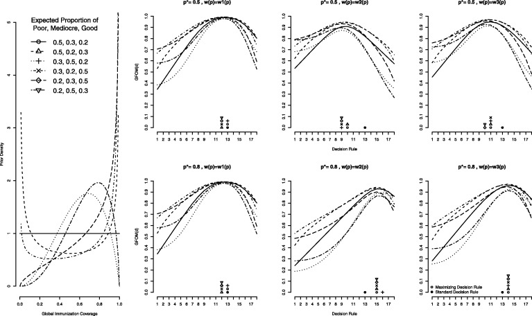
We consider six different underlying Beta distributions obtained by permuting the expected proportion of Poor (p ≤ 0.50), Mediocre (0.50 < p ≤ 0.80), and Good (p > 0.80) countries, starting with a uniform distribution (50% Poor, 30% Mediocre, and 20% Good). For example, the beta distribution that yields expected proportions of Poor, Mediocre and Good equal to 0.20, 0.30_, and 0.50, respectively, has parameters s₁ = 1.6035 and s₂ = 0.6028. The resulting six beta distributions are shown in Figure 3 (left).

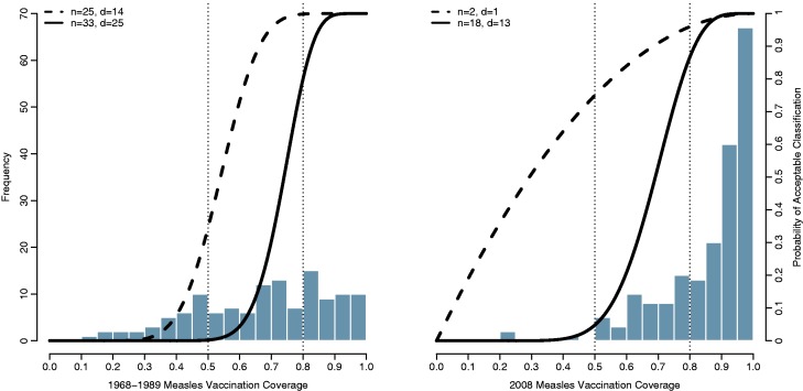
Figure 3.

Distribution of 1968–89 (left) and 2008 (right) UNICEF measles vaccination data. Overlaid are OC curves for various designs chosen using B-LQAS with weighting function w₃(.) with w₁ = 0.52, w₂ = 0.48 and minimum threshold k = 0.95

For each of the three weighting functions, we choose the input parameters w₁ and w₂ to be proportional to one minus the Producer and Consumer risks associated with the (18,13) LQAS design used by Sandiford (α = 0.133 and β = 0.048).⁵ That is, we let w₁ = (1−0.048)/(1−0.048 + 1−0.133) = 0.52 and w₂ = 1−w₁ = 0.48, placing slightly higher emphasis on correct classification of low coverage areas than high coverage ones. Lastly, we allow the programmatic threshold p* to equal either p_L = 0.50 or p_U = 0.80.

Application to UNICEF 1969–1989 and 2008 measles vaccination data

For our study of the UNICEF data, we first performed the identical analyses Sandiford performed but with the more recent vaccination data from 2008 and compared our results with Sandiford’s original findings.¹⁰ Table 1 contains the formulae for the quantities used in this analysis.

Table 1.

Possible outcomes of an LQAS test and metrics for design performance, contingent upon programmatic threshold, p*

	Actual Performance
	Poor p ≤ 0.50	Mediocre 0.50 < p < 0.80	Good p ≥ 0.80
LQAS Test Outcome	Unacceptable	a = E[OC(p) | p ≤ 0.50]	b = E[1-OC(p) | 0.50 < p < 0.80]	c = E[1-OC(p) | p ≥ 0.80]
	Acceptable	d = E[OC(p) | p ≤ 0.50]	e = E[OC(p) | 0.50 < p < 0.80]	f = E[OC(p) | p ≥ 0.80]
		Target Threshold
		For Detecting Poor (p* = pL)		For Detecting Good (p* = pU)
Performance Metrics	Sensitivity	a/(a + d)		f/(c + f)
	Specificity	(e + f)/(b + c + e + f)		(a + b)/(a + b + d + e)
	PPV	a/(a + b + c)		f/(d + e + f)
	NPV	(e + f)/(d + e + f)		(a + b)/(a + b + c)

We calculate the sensitivity, specificity, PPV and NPV for the 2008 distribution of measles vaccination coverage for LQAS considered as a test first for poor (p = p_L) and second for good (p = p_U) performance. These formulae are also given in Table 1.

Additionally, we apply B-LQAS to both the 1968–89 and the 2008 UNICEF data, employing as a weighting function w₃(·) with weights w₁ = 0.52 and w₂ = 0.48 (as before). Parameters for the assumed underlying beta distribution are fit via empirical Bayes.¹¹ We consider the case when p* is equal to 0.50 and 0.80. Based on the optimal decision rules identified by using B-LQAS, we re-calculate the expected sensitivity, specificity, PPV and NPV of the LQAS design and compare them with the same calculations using the (18, 13) design.

Lastly, we apply our proposed approach to choosing the optimal sample size and decision rule to the UNICEF data from both time periods assuming p* is equal to 0.50 or 0.80. We compare the implied OC curves from the resulting designs with the OC curve under traditional LQAS.

Results

Results of numerical study of B-LQAS

The GFOM* under various distributions and weighting schemes are presented in Figure 2 (right). When p* = 0.5, the optimal decision rules are uniformly 13 or less. As might be expected, in the case of weighting function w₁(·), which ignores the grey or Mediocre region, we see that an assumed uniform prior distribution leads to a decision rule of 13, the same rule used by Sandiford. In most other cases, when more than 20% of the prior mass is above the upper threshold, the optimal decision rule shifts to 12. Of course, the results are identical when p* = 0.80, because this weighting function does not consider the programmatic threshold.

Figure 2.

First column, density plots for six beta distributions with permuted expected proportions of Poor, Mediocre, and Good countries. Second, third, and fourth columns, GFOM plotted as a function of the decision rule for weighting functions w₁(.), w₂(.), and w₃(.) with assumed weights w₁ = 0.52 and w₂ = 0.48 and programmatic thresholds p* = 0.50 and 0.80. Points along the x-axis represent the maximizing decision rules for curves of corresponding point type and the solid dot indicates the decision rule under traditional LQAS

These findings contrast with the results obtained when using w₂(·); here the optimal decision rules reflect the programmatic thresholds. Namely, when p* = 0.50, the resultant optimal decision rules cluster near d = 9, which is unsurprisingly half of the sample size. Likewise, when p* = 0.80, the optimal decision rules are nearly all equal to 15.

Finally, with the weighting function w₃(·), the resulting decision rules when p* = 0.50 fall at either d = 11 or 12. When p* = 0.80, the optimal decision rule is uniformly equal to 14.

Results of application to UNICEF 1969–1989 and 2008 measles vaccination data

Expected classifications and performance metrics of the (18,13) LQAS design and the 1968–1989 and 2008 UNICEF measles vaccination distributions are presented in Table 2. The resulting values for specificity and PPV according to the 1968–89 distribution are low, with respective values 69.8% and 51.6% when p* = p_L, and 73.6% and 69.2% when p* = p_U. According to the 2008 distribution, the specificity increases to 86.8% and the PPV decreases to 10.6% when p* = p_L. The specificity decreases to 54.1% and the PPV increases to 86.4% when p* = p_U. Across time periods and irrespective of the choice of p*, the sensitivity and NPV are high, greater than 95% in most cases (NPV = 94.4% when p* = p_U in 2008 vaccination setting).

Table 2.

Distribution of measles vaccinations in 1968–89 and 2008, expected LQAS Classifications with n = 18 and d = 13, and expected performance metrics

		World Measles Vaccination Coverage
		1968–1989				2008
		Poor p ≤ 0.50	Mediocre 0.50 < p < 0.80		Good p ≥ 0.80	Poor p ≤ 0.50	Mediocre 0.50 < p < 0.80		Good p ≥ 0.80
LQAS Test Outcome	Unacceptable	30.5	26.9		1.8	3.0	23.6		1.6
	Acceptable	0.5	20.1		46.2	0	22.4		143.4
		For Detecting Poor (p* = pL)		For Detecting Good (p* = pU)		For Detecting Poor (p* = pL)		For Detecting Good (p* = pU)
Performance Metric	Sensitivity	98.5%		96.2%		99.4%		98.9%
	Specificity	69.8%		73.6%		86.8%		54.1%
	PPV	51.6%		69.2%		10.6%		86.4%
	NPV	99.3%		96.9%		100%		94.4%

Table 3 presents the resulting performance metrics when B-LQAS is used to choose the decision rule with a sample size fixed at n = 18 employing empirical Bayes estimates of s₁ = 2.54 and s₂ = 1.19 in 1968–1989 and s₁ = 5.13 and s₂ = 0.82 in 2008. When p* is equal to 0.50, GFOM is maximized at d = 10 for the 1968–1989 data, and at d = 9 for the 2008 data. For both time periods, the expected specificity increases to greater than 90%. PPV also increases, to 76.8% (from 51.6%) in 1968–89 and to 43.8% (from 10.6%) in 2008. When p*is equal to 0.80, GFOM is maximized at a decision rule of d = 14 and 13 in 1968–89 and 2008, respectively, which increases the specificity in the 1968–1989 period to 93.4% (from 73.6%) and PPV to 77.0% (from 69.2%). In all cases, the increase in specificity and PPV is at the expense of reduced sensitivity, particularly when p* = p_L. Across time periods and specifications of p*, the sensitivity never drops below 82.3%. To a lesser extent, we see a corresponding drop in NPV.

Table 3.

Expected LQAS performance metrics where decision rules are chosen to maximize GFOM with weighting function w₃(.) and weights w₁ = 0.52, w₂ = 0.48 for detecting both poor (p* = p_L) and good (p* = p_U) performance for a fixed sample size of n = 18

		World Measles Vaccination Coverage
		1968–1989		2008
		For Detecting Poor (p* = pL, d = 10)	For Detecting Good (p* = pU, d = 14)	For Detecting Poor (p* = pL, d = 9)	For Detecting Good (p* = pU, d = 13)
Performance Metric	Sensitivity	82.3%	90.6%	85.1%	98.9%
	Specificity	91.9%	93.4%	98.2%	54.1%
	PPV	76.8%	77.0%	43.8%	86.4%
	NPV	94.1%	93.5%	99.8%	94.4%

Table 4 shows the resulting performance metrics when both sample size and decision rules are chosen via B-LQAS. In order to achieve at least k = 0.95 expected probability of correct classification in the 1968–1989 data setting, the B-LQAS procedure recommends at least 25 observations with a decision rule of 14 when p* = 0.50 and at least 33 observations with a decision rule of 25 when p* = 0.80. In the 2008 data setting, only two observations with a decision rule of one are required when p* = 0.50. When p* = 0.80, the B-LQAS procedure selects the traditional design as optimal. OC curves for the B-LQAS optimal design are shown in Figure 3.

Table 4.

Expected LQAS performance metrics decision rules and sample sizes are chosen via B-LQAS with minimum threshold k = 0.95, weighting function w₃(.) and weights w₁ = 0.52, w₂ = 0.48 for detecting both poor where (p* = p_L)and good (p* = p_U) performance

		World Measles Vaccination Coverage
		1968–1989		2008
		For Detecting Poor (p* = pL, n = 25, d = 14)	For Detecting Good (p* = pU, n = 33, d = 25)	For Detecting Poor (p* = pL, n = 2, d = 1)	For Detecting Good (p* = pU, n = 18, d = 13)
Performance Metric	Sensitivity	86.8%	94.9%	49.1%	98.9%
	Specificity	91.9%	84.7%	96.8%	54.1%
	PPV	77.8%	79.2%	19.8%	86.4%
	NPV	95.5%	96.4%	99.2%	94.4%

Discussion

The results of our numerical study suggest that the choice of decision rule is quite sensitive to the underlying distribution of vaccination coverage. As we see in Table 3, even a small deviation in the decision rule can result in significant differences in the expected performance of the procedure. Likewise, the role of p* in choosing an optimal design is marked, resulting in wide variation in the recommended design. Yet, designs that favour correct classification of countries with high coverage are often chosen despite the fact that we weight low coverage classification more heavily (Figure 3). This is precisely the trade-off that one should make when there is prior knowledge suggesting that few countries have Poor coverage.

Our simple analysis of more recent measles vaccination data illustrates the importance of the distributional context on expected LQAS performance. The world made significant progress in child vaccination between 1989 and 2008.¹³ For this reason, when employing the same design in a different setting, we observe different performance characteristics. So had Sandiford used these more recent data, LQAS might have acquired a very different reputation. This nuance was clearly not lost on Sandiford, although it does not seem to have been clearly emphasized.

Using B-LQAS increases the expected specificity and PPV of the LQAS procedure for the UNICEF data, although in 2008, when p* = 0.50, the PPV remains low (43.8%). This result reflects observed distribution of the measles data in 2008, where only 1.5% of the countries had Poor coverage. In general, increases in specificity and PPV were accompanied by minimal, and in all cases probably acceptable, decreases in sensitivity and NPV.

The outlined approach to choosing the optimal sample size is generally conservative, resulting in recommended sample sizes greater than or equal to 18, except in 2008 when p* = 0.50. In this case, the recommended sample size is n = 2, a result that may seem questionable but is consistent with the low proportion of Poor countries in this dataset. We note, however, that we are limited in our ability to reflect all sources of variability in these data, such as survey sample size in each country and complex survey design. Appropriately characterizing these sources might result in more prior variability and likely an increase in the recommended sample sizes.

Two constraints of our work are the assumption that the target threshold, p*, is fixed, and its arbitrary identification with either the upper or the lower threshold. In practice this may not be realistic. For example, when LQAS is used as a tool to determine appropriate treatment strategy based on the prevalence of schistosomiasis infection, the choice of p* is driven by informed policy.^14–16 When used as a tool to evaluate neonatal tetanus eradication, p* represents the eradication threshold.¹⁷ Finally, when used in the context of a baseline survey, often neither p* nor the lower and upper thresholds are known before data are collected.^18–19 The choice of p*, as well as p_L and p_U, may well incorporate prior information to be optimally chosen, and not be fixed, as we assume here, but we leave that investigation to future work.

As is evident from the RC, LQAS is not a tool designed to distinguish well between Poor and Mediocre populations, for example. Rather, LQAS ensures that those populations with coverage at the extremes from the lower and upper thresholds are correctly identified with high probability. Incorporating prior information can inform LQAS design and improve its overall classification properties. Although some degree of tuning is always possible by relaxing constraints on Producer and Consumer risks or shifting the decision rule and/or sample size, the B-LQAS procedure is a valuable approach to incorporating prior information that can dramatically improve the aggregate performance of LQAS.

Supplementary Data

Supplementary data are available at IJE online.

Funding

This work was supported in part by the National Institutes of Health (R56 EB006195 to C.O. and M.P. and T32 ES015459 to C.O. and RO1, AI097015 to M.P.).

Conflict of interest: None declared.

Key messages.

• Expected performance is dependent upon the underlying distribution.

• Using all available information when designing an LQAS study can help to improve performance.

• Bayesian LQAS is a valuable approach to incorporating available information into LQAS design.

References

- 1.Robertson SE, Valadez JJ. Global review of health care surveys using lot quality assurance sampling (LQAS), 1984-2004. Soc Sci Med. 2006;63:1648–60. doi: 10.1016/j.socscimed.2006.04.011. [DOI] [PubMed] [Google Scholar]
- 2.Pagano M, Valadez JJ. Commentary: Understanding practical lot quality assurance sampling. Int J Epidemiol. 2010;39:69–71. doi: 10.1093/ije/dyp406. [DOI] [PMC free article] [PubMed] [Google Scholar]
- 3.Valadez JJ. Assessing Child Survival Programmes in Developing Countries: Testing Lot Quality Assurance Sampling. Boston: Harvard University Press; 1991. [Google Scholar]
- 4.Grant JP. The State of the World's Children 1991. Oxford: Oxford University Press; 1991. [Google Scholar]
- 5.Sandiford P. Lot quality assurance sampling for monitoring immunization programmes: cost-efficient or quick and dirty? Health Policy Plan. 1993;8:217–23. doi: 10.1093/heapol/8.3.217. [DOI] [PubMed] [Google Scholar]
- 6.Hutin YJF, Legros D, Owini V, et al. Trypanosoma brucei gambiense trypanosomiasis in Terego county, northern Uganda, 1996: a lot quality assurance sampling survey. Am J Trop Med Hyg. 2004;70:390–94. [PubMed] [Google Scholar]
- 7.Piot B, Mukherjee A, Navin D, et al. Lot quality assurance sampling for monitoring coverage and quality of a targeted condom social marketing programme in traditional and non-traditional outlets in India. Sex Transm Infect. 2010;86(Suppl 1):i56–61. doi: 10.1136/sti.2009.038356. [DOI] [PMC free article] [PubMed] [Google Scholar]
- 8.Stewart JC, Schroeder DG, Marsh DR, Allhasane S, Kone D. Assessing a computerized routine health information system in Mali using LQAS. Health Policy Plan. 2001;16:248–55. doi: 10.1093/heapol/16.3.248. [DOI] [PubMed] [Google Scholar]
- 9.Olives C, Pagano M. Bayes-LQAS: classifying the prevalence of global acute malnutrition. Emerg Themes Epidemiol. 2010;7:3. doi: 10.1186/1742-7622-7-3. [DOI] [PMC free article] [PubMed] [Google Scholar]
- 10.The State of the World's Children 2008. Child Survival. New York: UNICEF; 2008. [Google Scholar]
- 11.Berger J. Statistical Decision Theory. New York: Springer; 1980. [Google Scholar]
- 12.Olives C. 2010. Improving LQAS for monitoring and evaluation of health programmes in resource-poor settings. Ph.D. dissertation, Harvard School of Public Health, 2010. [Google Scholar]
- 13.World Health Organization. World Health Statistics Quarterly 2011. Geneva: World Health Organization; 2011. Available from: http://www.who.int/whosis/whostat/EN_WHS2011_Full.pdf (29 January 2013, date last accessed) [Google Scholar]
- 14.Brooker S, Kabatereine NB, Gyapong JO, Stothard JR, Utzinger J. Rapid mapping of schistosomiasis and other neglected tropical diseases in the context of integrated control programmes in Africa. Parasitology. 2009;136:1707–18. doi: 10.1017/S0031182009005940. [DOI] [PMC free article] [PubMed] [Google Scholar]
- 15.Brooker S, Kabatereine NB, Myatt M, Russell Stothard J, Fenwick A. Rapid assessment of Schistosoma mansoni: the validity, applicability and cost-effectiveness of the Lot Quality Assurance Sampling method in Uganda. Trop Med Int Health. 2005;10:647–58. doi: 10.1111/j.1365-3156.2005.01446.x. [DOI] [PMC free article] [PubMed] [Google Scholar]
- 16.Olives C, Valadez JJ, Brooker SJ, Pagano M. Multiple Category-Lot Quality Assurance Sampling: A New Classification System with Application to Schistosomiasis Control. PLoS Negl Trop Dis. 2012;6:e1806. doi: 10.1371/journal.pntd.0001806. [DOI] [PMC free article] [PubMed] [Google Scholar]
- 17.Stroh G, Birmingham M. Protocol for assessing neonatal tetanus mortality in the community using a combination of cluster and lot quality assurance sampling. Document WHO/V&B/02.05. Geneva: World Health Organization, Department of Vaccines and Biologicals; 2002. Available from: http://whqlibdoc.who.int/hq/2002/WHO_V&B_02.05.pdf (29 January 2013, date last accessed) [Google Scholar]
- 18.Valadez JJ, Weiss W, Leburg C, Davis R. Assessing community health programs: Using LQAS for baseline surveys and regular monitoring. St. Albans: Teaching-aids at Low Cost; 2003. [Google Scholar]
- 19.Valadez JJ, Devkota BR. Decentralized Supervision of Community Health Programmes Using LQAS in Two Districts in Southern Nepal. Boston: Management Sciences for Health; 2003. [Google Scholar]
Associated Data
This section collects any data citations, data availability statements, or supplementary materials included in this article.