

Abstract
System identification of physiological systems poses unique challenges, especially when the structure of the system under study is uncertain. Non-parametric techniques can be useful for identifying system structure, but these typically assume stationarity, and require large amounts of data. Both of these requirements are often not easily obtained in the study of physiological systems. Ensemble methods for time-varying, non-parametric estimation have been developed to address the issue of stationarity, but these require an amount of data that can be prohibitive for many experimental systems. To address this issue, we developed a novel algorithm that uses multiple short data segments. Using simulation studies, we showed that this algorithm produces system estimates with lower variability than previous methods when limited data are present. Furthermore we showed that the new algorithm generates time-varying system estimates with lower total error than an ensemble method. Thus, this algorithm is well suited for the identification of physiological systems that vary with time or from which only short segments of stationary data can be collected.
I. Introduction
System identification is a powerful analytical tool that allows for the mathematical quantification of dynamic systems using observed data. Non-parametric system identification is extremely useful in the analysis of physiological systems, as often there is insufficient a priori knowledge to generate a parametric model of the system from first principles. Classical non-parametric techniques require large data sets, and assume that the observed data are stationary. A major challenge in the study of physiological systems is that their dynamical properties vary with time or task, resulting in small data records, or data that can be considered stationary for only short periods of time. Thus special tools are required to characterize such systems using non-parametric system identification techniques.
Ensemble methods have previously been used to provide non-parametric descriptions of time-varying physiological systems [1–3]. These methods are useful for estimating non-stationary systems when a predictable time-varying change in the system dynamics occurs. This approach utilizes multiple repetitions of data with the same underlying time-varying behavior to generate non-parametric estimates of the system dynamics at each time point. Using this approach, previous studies measured the intrinsic mechanics [2, 3] as well as the stretch reflex response [1, 3] of the elbow and the ankle. These methods are well suited to estimate dynamics for systems where the same time-varying behavior can be easily and consistently repeated. However, this approach may require hundreds of realizations, resulting in an extremely time consuming and very demanding process. Furthermore, this approach may be inefficient if the time-varying dynamics are slower than the system dynamics, as the system dynamics will not vary greatly at each time point.
Parametric methods have also been used to estimate non-stationary behavior. These approaches have been used to estimate both mechanical [4, 5] and physiological systems [6–10]. However, parametric methods require knowledge of the system structure, thus may not be useful for physiological systems where little is known a priori. There are also a number of non-parametric frequency based methods for the estimation of non-stationary systems [11–13]. However, time-based methods are more appropriate in the estimation of certain physiological systems [3, 14].
In this paper, we present a novel algorithm that allows for the estimation of systems that are stationary for only short periods of time, or have a time-varying behavior that is slow relative to the time constants of the system under study. The presented algorithm also allows for the estimation of time-varying systems using a limited number of realizations. This was achieved by developing an algorithm that produces non-parametric estimates of system dynamics using multiple short segments of data. The validity and utility of this algorithm were evaluated using simulated data; the system that was simulated was the impedance of the human elbow. System identification has been extensively used in the analysis of human joint impedance [2, 3, 7, 14–18], making this a useful test system for evaluating algorithm performance. Our results demonstrate that this new approach is accurate, and more efficient than previous algorithms. They also identify the experimental regimes over which our new algorithm is most useful, thereby providing important guidelines for the system identification of physiological systems that are stationary for only short periods of time.
Part of this work has been presented previously at a conference [19].
II. Multi-Segment Identification Algorithm
A. Algorithm
One way to characterize a dynamic linear system is its impulse response function (IRF). The output of a system, y, can be computed as the discrete convolution of the input, x, and the IRF, h,
| (1) |
where i is the sample time, j is the lag of the IRF, Δt is the sampling increment, and M1 and M2 are the maximum and minimum lag respectively. The convolution shown in (1) is a time-varying convolution as h is a function of time, t.
An IRF can be estimated directly from the data by solving (1) for h. However, this computation can be quite intensive; alternatively the convolution equations can be re-written with auto (φxx) and cross-correlations (φxy) resulting in the following equation that is less computationally intensive to solve
| (2) |
Under stationary conditions, the cross-correlation can be computed by averaging across time (Eq. 3) [20].
| (3) |
In this equation, N is the number of points in each data record. Similarly the auto-correlation can be estimated as in (3), with y(i) being substituted by x(i). Under time-varying conditions with consistent time behavior, instantaneous correlations can be computed by averaging across multiple realizations, each assumed to have the same underlying time-varying behavior (Eq. 4).
| (4) |
Here, r is the realization number and R is the total number of realizations.
The time-varying cross-correlation is a powerful method as it provides an estimate of the correlation between the input and output at each time point. However, it requires many realizations to perform the required averaging, and may result in very long experimental times [2, 3]. Furthermore, if the underlying system is only slowly time-varying, or has short periods where it is nearly stationary, then the time-varying algorithm will be inefficient due to the presence of redundant computations. Instead, we propose to combine both time-invariant and time-varying correlations to estimate the behavior of the system during short data segments.
The combined approach was accomplished by averaging both along time within each short data segment, as well as across realizations. These multi-segment correlations can be formulated as
| (5) |
where t is the time at the middle of each short data segment, and N is the number of points in each segment.
Solving (2) for h(t, j) gives
| (6) |
where
and
This is a general solution for solving for h, and can be used in stationary or time-varying conditions. In the presence of a poor signal-to-noise ratio, solving (6) directly leads to large random error. Thus a pseudoinverse can be used, as proposed in [21].
B. Advantages of the Algorithm
Though the IRFs were estimated using correlation methods, it is shown in the Appendix that this is equivalent to IRFs estimated directly from the data using least-squares. As a result, the properties of least squares hold for these IRF estimates. Since the use of least-squares produces unbiased parameter estimates, the estimates produced by averaging numerous classical time-invariant IRFs or ensemble based time-varying IRFs [2] should be the same as that estimated by the multi-segment algorithm.
So, what is the benefit of the multi-segment algorithm? A derivation of the parameter variance—shown in the Appendix—shows a benefit in estimating the IRF of the system using the multi-segment algorithm
| (7) |
where σ2 is the variance of the IRF estimate for the multi-segment (MS), classical (C) and ensemble (E) algorithms, and M is the total number of lags. For example, given 20 realizations of 50 sample segments and an IRF of 9 lags, the classical and ensemble algorithms would produce estimates with variances that are 24% and 98% times larger than the multi-segment algorithm respectively. Thus, averaging IRFs estimated from classical or ensemble methods will lead to higher parameter variability than using the multi-segment algorithm. This effect will be greatest when small segments or few realizations are used, but becomes negligible with longer segments or greater number of realizations.
III. Simulation Studies
A number of simulation studies were run to evaluate the performance of the multi-segment algorithm. All focused on the estimation of human elbow impedance—the dynamic relationship between the position of the elbow and the torque acting about it—which was modeled parametrically by
| (8) |
where Tq is the output torque, θ is the input position, I is the joint inertia, B the viscosity, and K the stiffness. This is a typical representation, as used in a number of experimental studies [22, 23]. The first two studies used stationary data with a fixed set of model parameters. The first compared the performance of the algorithm to previously used classical [14] and ensemble algorithms [2]; the second evaluated the performance of our new algorithm for different data segment lengths and the number of total segments. The final simulation study used time-varying data. Specifically, the simulated elbow stiffness was varied in a sinusoidal manner to evaluate how well our algorithm could capture the dynamics of time-varying systems.
A. Simulation Methods
1) Simulation Model
The model shown in Fig. 1 was used to generate simulated data. The simulations were carried out using Simulink (The Mathworks inc.) with a fixed time step of 0.001 s. Each simulation set consisted of a series of realizations of the same length; each simulation in a set contained identical parameters, but different random values were used for the position and noise signals. The simulated position was a pseudo-random binary sequence (PRBS) with an amplitude of 0.03 rad, rate limited to ± 0.5 rad/s. This was selected to represent typical perturbations used in experimental studies [3, 14, 24]. The position was subsequently filtered at 40 Hz with an 8-pole Bessel filter. The output noise (Fig. 1) was low-pass filtered at 3 Hz with a 3-pole Bessel filter to accentuate the low frequency noise associated with voluntary intervention; it was then scaled to produce an output signal-to-noise ratio of 0 dB. Following the simulation, the data were filtered by a 40 Hz, 8th order Chebyshev filter and decimated to 100 Hz before the identification algorithms were applied.
Fig. 1.
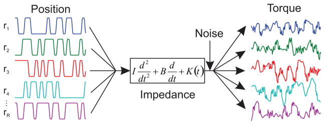
Schematic of simulations. Multiple realizations of simulated position signals were used to compute multiple realizations of simulated torque using the shown 2nd order differential.
2) Simulation 1: Comparison with Established Algorithms
The objective of the first simulations was to compare the performance of the multi-segment algorithm to that of the classical time-invariant and ensemble-based time-varying algorithms [2]. In this stationary simulation, 500 realizations of 8 s were simulated with the parameters of the impedance set to K = 150 Nm/rad, B = 2.2 Nm/rad/s and I = 0.13 kgm2.
To ensure that all algorithms had access to identical amounts of data, each used 20 randomly selected data segments with a length 0.5 s. Each segment was selected from a separate realization of the simulated system. The multi-segment algorithm estimated a single IRF from this set of 20 data segments; the classical algorithm computed an IRF for each segment, and the results were averaged to produce a single estimate; the ensemble approach computed a separate IRF for each time point, and these were averaged to yield a single estimate. This procedure was repeated 100 times, which we found to be a sufficient number of repetitions to allow for accurate estimates of the variability of the IRFs. Each repetition used different randomly selected realizations.
To evaluate the influence of the type of perturbation on the estimation process, we also considered filtered Gaussian white noise (FGWN), another common experimental choice [25]. This was generated using 2-pole Butterworth lowpass filter with a cutoff frequency of 5 Hz. The signal-to-noise ratio was matched to that used for the PRBS signal, as were all parameters used in the identification process.
Joint impedance IRFs are acausal representations of the system dynamics, and can be difficult to analyze visually [26]. Hence, the impedance IRFs were inverted to yield admittance IRFs, representing the dynamic relationship between a torque input and the resulting motion of the joint. This was accomplished by simulating the output of the impedance to filtered noise, and estimating an IRF where the output of the simulation was treated as the input to the IRF, and vice versa.
3) Simulation 2: Evaluation of the Performance of the Multi-Segment Algorithm
The second simulation study explored how the performance of the multi-segment algorithm varied with the number and length of the available data segments. The data used for this simulation were the same as in the previous simulation. Segment lengths from 0.01–2.0 s were considered, as were segment numbers from 1–200. All data were randomly selected from the available realizations. For each combination of segment length and number of realizations, the analysis was run 100 times.
The quality of the estimation was quantified in two ways. First the %VAF between the torque predicted by the algorithm (T̂q) and the simulated noise free torque (Tq) was computed as
| (9) |
Since the estimated torque was compared with the noise-free simulated torque, cross-validation was not required.
The quality of the algorithm was also evaluated by estimating the stiffness (K) of our simulated model. Stiffness, can be estimated directly by integrating the impedance IRF, and is not reliant on any parameter optimization routines.
4) Simulation 3: Estimation of Time-Varying Systems
One potential application of this multi-segment algorithm is the analysis of slowly time-varying systems. We assessed the utility of the algorithm for this application by simulating the system shown in Fig. 1, under conditions of sinusoidally varying K. 1000 realizations of 3 sinusoidal periods were simulated. In each realization, K varied according to (10), while I and B remained constant. Unique position and noise sequence were used for each realization.
| (10) |
This time-varying behavior was selected because it is much slower than the dynamics of the simulated impedance, but fast enough to preclude the use of classical time-invariant methods.
To analyze these simulations, the algorithm was run at each time point using sets of 25, 50 and 100 randomly selected realizations. The algorithm was evaluated for segment lengths that varied from 0.05–1.0 times the period of the time-varying behavior; segments were centered at each time point in the selected realizations. Stiffness estimates were generated as in the previous subsection. This process was repeated for 100 randomly selected data sets to obtain estimates of the random error (eR), bias error (eB), and total error (eT) associated with each estimate. These errors were computed as follows:
| (11) |
K̂(t, s) is the stiffness estimated at time point t and data set s, K(t) is the simulated stiffness, is the mean of K̂(t,s) across all data sets (12), Δt is sampling increment and S is the total number of data sets evaluated.
| (12) |
B. Simulation Results
1) Simulation 1: Comparison with Established Algorithms
The first simulation study compared the performance of the multi-segment algorithm to that of the classical time-invariant and ensemble based time-varying algorithms.
For the FGWN input, all three algorithms produced unbiased estimates of the admittance (Fig. 2 left column). However the multi-segment algorithm computed IRFs with lower variability (average st. dev = 0.008 rad/Nm/s) compared to the classical (average st.dev = 0.010 rad/Nm/s) and ensemble (average st. dev = 0.012 rad/Nm/s) algorithms. These results are in general agreement with (7) as the multi-segment algorithm estimated admittance with the lowest variability of the three algorithms, and the classical algorithm produced estimates with slightly lower variability than the ensemble algorithm.
Fig. 2.

Joint admittance IRFs. Admittance IRFs estimated using the a) classical, b) ensemble and c) multi-segment algorithms with both FGWN (left column) and PRBS (right column) inputs. Shaded areas show ± 2 standard deviations for each algorithm and black-dashed lines show the true IRF used in the simulations.
The advantage of the multi-segment algorithm becomes even more pronounced with the PRBS data (Fig. 2 right column). Not only did the multi-segment algorithm produce estimates with lower variability, but it also produced unbiased estimates. This was in contrast to the classical algorithm, which produced biased estimates for the simulated conditions. This bias arose due to the likelihood that a number of the input signals were ill conditioned, a distinct possibility when using short segments of PRBS data, as some individual segments may contain few transitions.
2) Simulation 2: Evaluation of the Performance of the Multi-Segment Algorithm
Our second simulation study evaluated how the number of available realizations, and the number of data points in each realization influenced algorithm performance. Both the %VAF (Fig. 3a) and the standard deviation of the estimated stiffness parameter, K (Fig. 3b) showed improvement with increasing amounts of data; however the %VAF reached high levels (~95%) after only approximately 2500 data points, whereas the standard deviation reached high levels (~5%) after 10000 data points. Thus, even though only small improvement were seen in the %VAF when using increasing number of longer segments, the decrease in the variability of the estimated K was greatly enhanced by the availability of more data.
Fig. 3.

Performance of multi-segment algorithm. %VAF (a) and standard deviation (b) of the stiffness estimate for multi-segment algorithm as a function of segment length and number of realizations.
For the majority of the combinations shown in Fig. 3 there was no difference as to the performance of the algorithm with respect to the origin of the amount of data. That is to say the algorithm performs equally well when using 150 realizations of 0.5 s data or 50 realizations of 1.5 s data.
3) Simulation 3: Estimation of Time-Varying Systems
Our third simulation addressed the challenge of selecting proper segment lengths when dealing with time-varying systems. Longer data segments will benefit from better algorithm performance, as demonstrated in the previous section, but may miss the time-varying behavior. Shorter data segments will result in estimates that capture the time-varying behavior but will have increased random error. To assess this issue, we evaluated the accuracy of the algorithm in estimating time-varying stiffness using segments of different lengths. Fig. 4a shows an example of the estimates generated when 100 realizations of time-varying data were segmented into 3 different lengths. We found that segments with a length of 0.1 times the period of the simulated sinusoidal time variation produced estimates of K that had little bias but a large amount of variability (Fig. 4a, top). Using segment lengths of 0.4 times the period resulted in estimates of K with greater bias, but decreased variability (Fig. 4a, middle). Finally, when the segments were 0.7 of the period, the algorithm estimated K with the least variability, but substantial bias (Fig 4a, bottom).
Fig. 4.

Estimation of time-varying behavior. a) K (solid) estimated from data of three different segment lengths with 2 standard deviations (shaded region) along with simulated values (black-dashed) b) Bias (solid), random (dotted) and total (dashed) error in estimating time-varying stiffness as a function of segment length when estimating time using 25 (blue), 50 (green) and 100 (red) realizations. Black circles demarcate the three segment lengths shown in part a.
The optimal segment length, quantified by the total estimation error, varied with the available number of realizations (Fig. 4b). Random error, bias error and total error all varied as a function of both segment length and the number of realizations. In general, we found that as segment length increased random error decreased and bias error increased. However, there was a point in between the two extremes where the total error reached a local minimum. As expected, increasing the number of realizations available to the algorithm resulted in estimates of K with decreased random error and no change in bias error, thus shifting the segment length at which total error reached a local minimum. The previously used ensemble algorithm [2] used segments that were one sample long. Thus when data are limited and noise is substantial, the multi-segment algorithm estimates time-varying systems with lower total error than the established ensemble algorithm.
IV. Discussion
The goal of this study was to develop and evaluate a novel algorithm for obtaining non-parametric estimates of physiological systems that are stationary for only short periods of time. Our approach uses multiple realizations of short data segments. In addition to situations in which only short data segments are available, this algorithm can also be applied to slowly time-varying systems. Our approach can be contrasted with classical time-invariant methods that use lengthy single realizations of stationary data, and ensemble time-varying methods that use numerous realizations of rapidly varying behaviors. We assessed the algorithm by quantifying its performance in estimating joint impedance, a physiological system that has been studied in detail previously [2, 3, 7, 10, 14–18, 24, 27–30]. Using simulations we determined that the new algorithm could produce impedance IRFs with lower variability and less bias than classical time-invariant and ensemble-based time-varying approaches. While the novel algorithm could estimate joint impedance with even small amounts of data, it required substantially more data to produce reliable estimates of the stiffness parameter corresponding to the static component of impedance. Finally, we showed that using numerous realizations of short data segments, the algorithm generates time-varying system estimates with lower total error than previously used time-varying ensemble methods [2, 3, 21]
A. Advantages of Multi-Segment Algorithm
The main advantage of the multi-segment algorithm is its ability to estimate system dynamics with lower variability than classical methods when using multiple short segments of data. It is possible to produce multiple system estimates using classical time-invariant methods on each realization and average the result, with (7) showing the expected parameter variability. For data sets where the data length is much greater than the number of lags of the IRF, the advantage of the multi-segment algorithm is negligible. However when the length of data is not substantially greater than the number of lags, the multi-segment will produce system dynamics estimates with lower variability. We demonstrated this in Simulation 1; the standard deviation was lower for the estimates generated by the multi-segment than the classical or ensemble algorithms.
This decrease in parameter variability is expected, but there is another practical benefit to the algorithm. In any given realization, there is a possibility that the there is insufficient power to correctly estimate the system. If even one realization has insufficient power, using the average of time-invariant IRF method would result in an average IRF that may be extremely biased. This possibility of insufficient power in individual realizations is much greater with the PRBS signal, a common experimental choice due to its increased power for a given peak-to-peak amplitude as compared to Gaussian noise [17]. In Simulation 1, the segment lengths (0.5 s) were relatively short in comparison to the switching rate of the PRBS (0.15 s). Thus, it is expected that in an ensemble of 20 realizations 2 or 3 realizations are likely to be ill conditioned, resulting in 2 or 3 IRFs with extreme errors that could add substantial bias to the average IRF. In such conditions, the multi-segment algorithm has substantial advantages.
This approach is especially useful for physiological systems, which tend to require more data than electrical or mechanical systems. This arises from the low signal-to-noise ratios often encountered in the study of physiological systems, the limitations on the properties of the input perturbations than can be applied, as well as the need for non-parametric approaches when studying systems with unknown structure. Though the requirement for data is higher, the accessibility to stationary data from physiological systems is often lower, due to issues such as the fatigue. If the non-stationary behavior can be repeated in a predictable manner then the system can be treated as a time-varying system. However, this requires the subject to perform the same time-varying change many hundreds of times, a demanding and time consuming task [2, 3]. Thus, maximizing the utilization of the acquired data is essential for physiological system identification and this algorithm is well suited for this purpose.
B. Estimation of Time-Varying Systems
We showed that increasing the segment length and number of realizations improved performance, but for time-varying systems, making segments too long may result in inaccurate estimates of the time-varying behavior. So, how does one choose the proper values for segment length and number of realizations? We found that for each data set (realizations = 25, 50, 100) there was some value where the total error reached a local minimum (0.45, 0.35 and 0.3 of the period respectively). Computing this optimal segment length a priori may not be feasible, as even predicting the random error with a white input was quite challenging (Appendix B). A more practical solution may be to run a limited set of simulations, and use some a priori assumptions to approximate the optimal length over a wide array of conditions.
The results of the time-varying simulation demonstrate that the multi-segment algorithm produces estimates of time-varying systems with less error than the established ensemble algorithm. The ensemble algorithm is equivalent to the multi-segment algorithm when the segments are one sample each—0.01 s in this case. Thus, under the situations simulated here—low SNR and limited number of realizations—that are typical for physiological systems, estimating slowly time-varying system is more effective with the multi-segment algorithm.
C. Applications of the Algorithm
We foresee a number of applications for the multi-segment algorithm presented in this paper. One would be to estimate the dynamics of time-varying systems as detailed thoroughly in this paper. For example, joint impedance has been extensively studied under stationary posture [24, 28]; yet few have thoroughly examined how joint impedance varies with natural movements [7, 22, 31]. Estimating impedance during movement may provide insight into the neural control of movement [32, 33]. It may also provide information of the mechanics of the joint that will help with the design of biomimetic prostheses [34, 35].
Another application would be to estimate the state of systems that remain stationary for only short periods of time. For example, there is a challenge associated with measuring joint impedance at high torque levels, since levels above approximately 30% of maximum voluntary contraction can only be maintained for short time periods. As a result, most studies have estimated joint mechanics at relatively low levels of voluntary contraction [18, 36, 37]. Estimating impedance at high torque levels would be useful for understanding how joint mechanics are regulated during impact, and also could be used to better understand the relative importance of muscle and tendon mechanics within these regimes [38, 39]. Similarly, these methods could also be used to estimate joint impedance in other transients states such as in preparation to move, or in the preparation for an impact. In general, this method is valuable to estimate any system where the state of interest is too short to acquire sufficient data to accurately estimate the system.
The major advantage of non-parametric algorithms is their ability to estimate system dynamics without a priori knowledge of the structure of the system. Thus, they are especially useful for physiological applications. Ultimately, the algorithm we developed would provide insight into structure of the system, which would then allow for the use of parametric techniques [4–9, 40, 41] that can estimate system dynamics with much less data.
Acknowledgments
This work was supported by the National Institutes of Health (grant R01 NS053813).
Biographies

Daniel Ludvig (S’06-M’11) received the B.Sc. degree in physiology and physics in 2003, the M.Eng. degree in biomedical engineering in 2006 and the Ph.D. degree in biomedical engineering in 2010 from McGill University, Montreal, QC, Canada.
He is currently a Postdoctoral Fellow in the Sensory Motor Performance Program at the Rehabilitation Institute of Chicago, Chicago, IL, and a Research Affiliate with the Department of Biomedical Engineering at Northwestern University, Evanston, IL. He also acts as a Research Consultant for the Institut de Recherche Robert-Sauve en Sante et Sécurité du Travail, Montreal, Quebec, Canada. His research interests focus on the use of system identification in investigating human motor control systems. In particular, his research involves modeling how humans maintain posture and control movements of their limbs.
Dr. Ludvig is a Member of the IEEE, as well as the Society for Neuroscience.

Eric J. Perreault (S’96–M’00) received his B.Eng and M. Eng degrees in electrical engineering from McGill University, Montreal, QC, Canada in 1989 and 1991, respectively. After working in industry for 4 years, he received the Ph.D. degree in biomedical engineering from Case Western Reserve University, Cleveland, OH, in 2000.
He is currently an Associate Professor at Northwestern University, with appointments in the Department of Biomedical Engineering and the Department of Physical Medicine and Rehabilitation. He also is a member of the Sensory Motor Performance Program at the Rehabilitation Institute of Chicago, where his laboratory is located. From 2000–2002, he was a Postdoctoral Fellow in the Department of Physiology at Northwestern University. In 2010, he was a Visiting Professor at ETH Zürich. His current research focuses on understanding the neural and biomechanical factors involved in the control of multi-joint movement and posture and how these factors are modified following neuromotor pathologies such as stroke and spinal cord injury. The goal is to provide a scientific basis for understanding normal and pathological motor control that can be used to guide rehabilitative strategies and user interface development for restoring function to individuals with motor deficits. Current applications include rehabilitation following stroke and tendon transfer surgeries, and user interfaces for neuroprosthetic control.
Prof. Perreault serves as an Associate Editor for the IEEE Transactions on Neural Systems and Rehabilitation Engineering, and serves on the editorial boards for the Journal of Motor Behavior and the Journal of Motor Control. He also is a member of the IEEE Technical Committee on Rehabilitation Robotics.
Appendix
A. Correlation and least-squares IRF estimates
In the text we showed the estimation of the multi-segment IRF using correlation based methods. This method is identical to the least-squares method, thus it too has all the properties of least-squares estimates.
Similar to (1), the output of the system for any given realization can be computed using a discrete convolution
| (14) |
where i is a time point during the stationary period, thus
Eq. (14) can be rewritten in a matrix formulation as
| (15) |
where
and
Computing the output for all realizations results in the following equation
| (16) |
where
and
In the presence of noise, (16) cannot be solved for h directly; rather h can be estimated using least-squares linear regression
| (17) |
Computing XTY gives
| (18) |
where
Resulting in an expression that is identical to the cross-correlation shown in (6) except for the normalization.
Similarly computing XTX gives
| (19) |
where
Substituting in k = k2 − k1 and t* = t − k1 gives
where
| (20) |
Resulting in the same matrix of auto-correlations as in (7) except for the normalization. The normalization from the auto and cross-correlations cancel out, thus the correlation method of solving for the IRF is identical to the least-squares method, and therefore has all the properties of least-squares estimates.
B. Parameter variance estimates
The variance of least-squares parameter estimates is
| (21) |
where is the noise variance, and C(j) is the entry on the jth row and jth column of (XTX)−1.
For a Gaussian white input with a variance of 1
| (22) |
where di is random variable from a χ2 distribution with n degrees of freedom, and bij is the sum of n random variables from a product of normal distributions, n is the total number of data points and M is the total number of lags. Inverting (22) and computing the expected value of each diagonal entry analytically is not reasonable; rather we ran Monte-Carlo simulation where we found that for up to 100 lags each diagonal entry in (XTX)−1 can be approximated by
| (23) |
Thus, the parameter variance of the estimates generated by the multi-segment algorithm is
| (24) |
For a single IRF estimated by the classical or ensemble algorithms, the parameter variance is given by
| (25) |
Averaging multiple classical IRFs results in parameter variance of
| (26) |
A similar process shows that
| (27) |
Contributor Information
Daniel Ludvig, Email: daniel.ludvig@mail.mcgill.ca, Sensory Motor Performance Program, Rehabilitation Institute of Chicago, and the Department of Biomedical Engineering, Northwestern University, Chicago, IL 60611 USA (phone: 312-238-0956; fax: 312-238-2208).
Eric J. Perreault, Email: e-perreault@northwestern.edu, Department of Biomedical Engineering and the Department of Physical Medicine and Rehabilitation at Northwestern University, Chicago, IL 60611 USA, and also with Sensory Motor Performance Program, Rehabilitation Institute of Chicago, Chicago, IL 60611 USA.
References
- 1.Soechting JF, et al. Time-varying properties of myotatic response in man during some simple motor tasks. J Neurophysiol. 1981 Dec;46:1226–43. doi: 10.1152/jn.1981.46.6.1226. [DOI] [PubMed] [Google Scholar]
- 2.MacNeil JB, et al. Identification of time-varying biological systems from ensemble data. IEEE Trans Biomed Eng. 1992 Dec;39:1213–25. doi: 10.1109/10.184697. [DOI] [PubMed] [Google Scholar]
- 3.Ludvig D, et al. Identification of time-varying intrinsic and reflex joint stiffness. IEEE Trans Biomed Eng. 2011 Jun;58:1715–23. doi: 10.1109/TBME.2011.2113184. [DOI] [PubMed] [Google Scholar]
- 4.Poulimenos AG, Fassois SD. Parametric time-domain methods for non-stationary random vibration modelling and analysis - A critical survey and comparison. Mechanical Systems and Signal Processing. 2006 May;20:763–816. [Google Scholar]
- 5.Spiridonakos MD, Fassois SD. Parametric identification of a time-varying structure based on vector vibration response measurements. Mechanical Systems and Signal Processing. 2009 Aug;23:2029–2048. [Google Scholar]
- 6.Xu Y, Hollerbach JM. Identification of human joint mechanical properties from single trial data. IEEE Trans Biomed Eng. 1998 Aug;45:1051–60. doi: 10.1109/10.704874. [DOI] [PubMed] [Google Scholar]
- 7.Bennett DJ, et al. Time-varying stiffness of human elbow joint during cyclic voluntary movement. Exp Brain Res. 1992;88:433–42. doi: 10.1007/BF02259118. [DOI] [PubMed] [Google Scholar]
- 8.Piovesan D, et al. Measuring multi-joint stiffness during single movements: numerical validation of a novel time-frequency approach. PLoS One. 2012;7:e33086. doi: 10.1371/journal.pone.0033086. [DOI] [PMC free article] [PubMed] [Google Scholar]
- 9.Tsatsanis MK, Giannakis GB. Time-Varying System-Identification and Model Validation Using Wavelets. Ieee Transactions on Signal Processing. 1993 Dec;41:3512–3523. [Google Scholar]
- 10.Lacquaniti F, et al. Time-varying mechanical behavior of multijointed arm in man. J Neurophysiol. 1993 May;69:1443–64. doi: 10.1152/jn.1993.69.5.1443. [DOI] [PubMed] [Google Scholar]
- 11.Hammond JK, White PR. The analysis of non-stationary signals using time-frequency methods. Journal of Sound and Vibration. 1996 Feb 29;190:419–447. [Google Scholar]
- 12.Lataire J, Pintelon R. Frequency-domain weighted non-linear least-squares estimation of continuous-time, time-varying systems. Iet Control Theory and Applications. 2011 May;5:923–933. [Google Scholar]
- 13.Lataire J, et al. Non-parametric estimate of the system function of a time-varying system. Automatica. 2012 Apr;48:666–672. [Google Scholar]
- 14.Kearney RE, et al. Identification of intrinsic and reflex contributions to human ankle stiffness dynamics. IEEE Trans Biomed Eng. 1997 Jun;44:493–504. doi: 10.1109/10.581944. [DOI] [PubMed] [Google Scholar]
- 15.Zhang LQ, Rymer WZ. Simultaneous and nonlinear identification of mechanical and reflex properties of human elbow joint muscles. IEEE Trans Biomed Eng. 1997 Dec;44:1192–209. doi: 10.1109/10.649991. [DOI] [PubMed] [Google Scholar]
- 16.Ludvig D, Kearney RE. Real-time estimation of intrinsic and reflex stiffness. IEEE Trans Biomed Eng. 2007 Oct;54:1875–84. doi: 10.1109/TBME.2007.894737. [DOI] [PubMed] [Google Scholar]
- 17.Kearney RE, Hunter IW. System identification of human joint dynamics. Crit Rev Biomed Eng. 1990;18:55–87. [PubMed] [Google Scholar]
- 18.Perreault EJ, et al. Effects of voluntary force generation on the elastic components of endpoint stiffness. Exp Brain Res. 2001 Dec;141:312–23. doi: 10.1007/s002210100880. [DOI] [PubMed] [Google Scholar]
- 19.Ludvig D, Perreault EJ. Estimation of joint impedance using short data segments. Conf Proc IEEE Eng Med Biol Soc. 2011 Aug;2011:4120–3. doi: 10.1109/IEMBS.2011.6091023. [DOI] [PMC free article] [PubMed] [Google Scholar]
- 20.Bendat JS, Piersol AG. Random data: analysis and measurement procedures. 3. New York: Wiley; 2000. [Google Scholar]
- 21.Lortie M, Kearney RE. Identification of physiological systems: estimation of linear time-varying dynamics with non-white inputs and noisy outputs. Med Biol Eng Comput. 2001 May;39:381–90. doi: 10.1007/BF02345295. [DOI] [PubMed] [Google Scholar]
- 22.Popescu F, et al. Elbow impedance during goal-directed movements. Exp Brain Res. 2003 Sep;152:17–28. doi: 10.1007/s00221-003-1507-4. [DOI] [PubMed] [Google Scholar]
- 23.Trumbower RD, et al. Use of self-selected postures to regulate multi-joint stiffness during unconstrained tasks. PLoS One. 2009;4:e5411. doi: 10.1371/journal.pone.0005411. [DOI] [PMC free article] [PubMed] [Google Scholar]
- 24.Mirbagheri MM, et al. Intrinsic and reflex contributions to human ankle stiffness: variation with activation level and position. Exp Brain Res. 2000 Dec;135:423–36. doi: 10.1007/s002210000534. [DOI] [PubMed] [Google Scholar]
- 25.Pfeifer S, et al. Model-Based Estimation of Knee Stiffness. IEEE Trans Biomed Eng. 2012 Jul 11; doi: 10.1109/TBME.2012.2207895. [DOI] [PMC free article] [PubMed] [Google Scholar]
- 26.Westwick D, Perreault E. Estimates of acausal joint impedance models. IEEE Trans Biomed Eng. 2012 Aug 15; doi: 10.1109/TBME.2012.2213339. [DOI] [PMC free article] [PubMed] [Google Scholar]
- 27.Ludvig D, et al. Voluntary modulation of human stretch reflexes. Exp Brain Res. 2007 Nov;183:201–13. doi: 10.1007/s00221-007-1030-0. [DOI] [PubMed] [Google Scholar]
- 28.Zhang LQ, et al. In vivo human knee joint dynamic properties as functions of muscle contraction and joint position. J Biomech. 1998 Jan;31:71–6. doi: 10.1016/s0021-9290(97)00106-1. [DOI] [PubMed] [Google Scholar]
- 29.Sinkjaer T, et al. Muscle stiffness in human ankle dorsiflexors: intrinsic and reflex components. J Neurophysiol. 1988 Sep;60:1110–21. doi: 10.1152/jn.1988.60.3.1110. [DOI] [PubMed] [Google Scholar]
- 30.Kirsch RF, Kearney RE. Identification of time-varying stiffness dynamics of the human ankle joint during an imposed movement. Exp Brain Res. 1997 Mar;114:71–85. doi: 10.1007/pl00005625. [DOI] [PubMed] [Google Scholar]
- 31.Latash ML, Gottlieb GL. Reconstruction of shifting elbow joint compliant characteristics during fast and slow movements. Neuroscience. 1991;43:697–712. doi: 10.1016/0306-4522(91)90328-l. [DOI] [PubMed] [Google Scholar]
- 32.Gomi H, Kawato M. Human arm stiffness and equilibrium-point trajectory during multi-joint movement. Biol Cybern. 1997 Mar;76:163–71. doi: 10.1007/s004220050329. [DOI] [PubMed] [Google Scholar]
- 33.Burdet E, et al. The central nervous system stabilizes unstable dynamics by learning optimal impedance. Nature. 2001 Nov 22;414:446–9. doi: 10.1038/35106566. [DOI] [PubMed] [Google Scholar]
- 34.Hansen AH, et al. The human ankle during walking: implications for design of biomimetic ankle prostheses. J Biomech. 2004 Oct;37:1467–74. doi: 10.1016/j.jbiomech.2004.01.017. [DOI] [PubMed] [Google Scholar]
- 35.Ha KH, et al. Volitional control of a prosthetic knee using surface electromyography. IEEE Trans Biomed Eng. 2011 Jan;58:144–51. doi: 10.1109/TBME.2010.2070840. [DOI] [PubMed] [Google Scholar]
- 36.Gomi H, Osu R. Task-dependent viscoelasticity of human multijoint arm and its spatial characteristics for interaction with environments. J Neurosci. 1998 Nov 1;18:8965–78. doi: 10.1523/JNEUROSCI.18-21-08965.1998. [DOI] [PMC free article] [PubMed] [Google Scholar]
- 37.Franklin DW, Milner TE. Adaptive control of stiffness to stabilize hand position with large loads. Exp Brain Res. 2003 Sep;152:211–20. doi: 10.1007/s00221-003-1540-3. [DOI] [PubMed] [Google Scholar]
- 38.Cui L, et al. Modeling short-range stiffness of feline lower hindlimb muscles. J Biomech. 2008;41:1945–52. doi: 10.1016/j.jbiomech.2008.03.024. [DOI] [PMC free article] [PubMed] [Google Scholar]
- 39.Hu X, et al. Muscle short-range stiffness can be used to estimate the endpoint stiffness of the human arm. J Neurophysiol. 2011 Apr;105:1633–41. doi: 10.1152/jn.00537.2010. [DOI] [PMC free article] [PubMed] [Google Scholar]
- 40.Dos Santos PL, et al. Linear Parameter-Varying System Identification: New Developments and Trends. World Scientific Publishing Company; 2012. [Google Scholar]
- 41.Toth R. Modeling and Identification of Linear Parameter-Varying Systems. Springer; 2010. [Google Scholar]