

Abstract
Estimates of joint or limb impedance are commonly used in the study of how the nervous system controls posture and movement, and how that control is altered by injury to the neural or musculoskeletal systems. Impedance characterizes the dynamic relationship between an imposed perturbation of joint position and the torques generated in response. While there are many practical reasons for estimating impedance rather than its inverse, admittance, it is an acausal representation of the limb mechanics that can lead to difficulties in interpretation or use. The purpose of this study was to explore the acausal nature of nonparametric estimates of joint impedance representations to determine how they are influenced by common experimental and computational choices. This was accomplished by deriving discrete-time realizations of first-and second-order derivatives to illustrate two key difficulties in the physical interpretation of impedance impulse response functions. These illustrations were provided using both simulated and experimental data. It was found that the shape of the impedance impulse response depends critically on the selected sampling rate, and on the bandwidth and noise characteristics of the position perturbation used during the estimation process. These results provide important guidelines for designing experiments in which nonparametric estimates of impedance will be obtained, especially when those estimates are to be used in a multistep identification process.
Index Terms: Discrete-time, joint dynamics, parametric model, sampling, system identification, time domain, two-sided impulse response
I. Introduction
The dynamics of a joint are described by the relationship between torques applied to that joint and the positions, velocities, and accelerations generated in response. There is a causal relationship, known as the compliance, or the admittance, between the applied torques and the resulting motions. This relationship can be quantified for single [1]–[4] and multijoint systems [5]–[7]. The dynamics of individual joints typically can be characterized as second-order systems with impulse responses that oscillate and decay exponentially. Quantification of these dynamics has proven to be a useful tool for assessing the properties of the neuromuscular system, and how those properties are regulated across different tasks and disease states. For example, linear and nonlinear models of single-joint and multijoint systems have been used to study adaptation to different mechanical environments [8], and changes in the regulation of limb mechanics following neuromuscular disease including spinal cord injury [9] and stroke [10].
System identification techniques [11] can be used to construct models of joint dynamics from time series measurements of joint torque and joint position. However, it is common in experimental studies to control joint position and measure the resulting torques [3], [4], [12]–[15]. This is because position-controlled actuators are easier to control over a wide bandwidth than force-controlled actuators, allowing the joint dynamics to be estimated using open-loop rather than closed-loop identification algorithms [4], [16]. Furthermore, very stiff position-controlled actuators can be used to experimentally separate reflex and intrinsic muscle contributions to joint stiffness [12], [17], [18], providing further insight regarding the physiological mechanisms contributing to the net joint dynamics. The use of position inputs gives rise to the stiffness formulation of joint dynamics, often also described in the literature as dynamic stiffness or impedance. In the time domain, joint impedance is represented as a two-sided impulse response function (IRF) [19], which has nonzero values at negative time-lags. This representation corresponds to an acausal system, as the impulse response starts before the impulse arrives.
Unlike causal admittance IRFs, acausal impedance IRFs can be difficult to interpret. The shape and time course of these acausal IRFs depends not only on the properties of the joint dynamics, but also on those of the inputs used to perturb the joint, the noise in the corresponding measurements and the rate at which the data are sampled. These dependences are particularly important in multistep identification algorithms that depend on the shape and time course of the impedance IRF. Such techniques have proved useful for estimating reflex contributions to joint dynamics [12], although only for a restricted class of imposed perturbations. A better understanding of the technical and mathematical factors contributing to the estimates of joint impedance may contribute to their use in a broader range of applications.
Note that in a strict analogy with their electrical definitions, the impedance and its inverse, the admittance, are relationships between the velocity (analogous to current) and force (analogous to voltage). However, in the robotics and motor control literatures, these terms are often used to refer to relationships between force and position, instead of velocity.
The purpose of this study was to present a thorough analysis of the impedance IRF and the practical difficulties inherent in its estimation. Specifically, we have derived a theoretical description of the shape of an impedance IRF and how that shape is influenced by experimentally relevant parameters including sampling rate, input bandwidth, and noise. These theoretical analyses are compared to simulated and experimental results to demonstrate how they influence the estimates made under typical experimental conditions. Preliminary results of this study have previously been published in abstract form [20].
II. Background
In many cases, when the effects of reflexes are insignificant, the admittance of a joint can be approximated using a second-order linear system
| (1) |
where Θ(s) is the Laplace transform of the joint angle, T (s) is the transform of the joint torque, and I, B, and K are the inertia, damping, and spring constants, respectively. Note that the transfer function in (1) is proper, in that it has more poles than zeros. As such, it can be readily transformed into the time domain, and then discretized.
To obtain the impedance formulation, one inverts the equation of motion. Transforming the result back to the time domain produces an equation that is linear in the parameters.
| (2) |
However, using (2) as a model requires computing the first and second time derivatives, θ̇(t) and θ̈(t), respectively, of the joint angle, θ(t). These computations result in an acausal representation of the joint mechanics, as described in Section III-A. Understanding this representation and how it is influenced by experimental and computational choices is necessary when using approaches that specifically require an impedance representation in the time domain [12].
A. Experimental Considerations
Experiments for estimating joint impedance typically use a servo motor to perturb the position of the joint in a controlled manner. Because high-fidelity position servos are reasonably easy to implement, they have been used in this context for several decades [4]. Provided that the position servo has a stiffness that is one or more orders of magnitude stiffer than the joint being tested, treating the measured position as the system input produces a reasonable estimate of the joint impedance. Furthermore, reflexes, which produce muscle contractions in reaction to stretches applied to the tendon or muscle, can be modeled as parallel pathways to the linear joint impedance term [12].
The characteristics of the servo strongly influence the experimental outcomes. This can be seen by considering a simplified representation of an impedance estimation experiment (see Fig. 1). In this figure, the servo-controlled actuator is represented by a constant gain Ka symbolic of a servo with a bandwidth that is far greater than that of the attached limb. Large values of Ka represent stiff position servos, whereas lower values represent more compliant servos. Voluntary contractions, which create torques Tv (s), have been included as they can be a significant source of noise in many experimental paradigms.
Fig. 1.
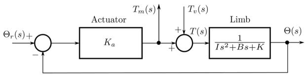
Simplified block diagram of an experimental apparatus used to study limb dynamics. The Laplace transforms of the measured torque and position are given by Tm (s) and Θ(s), respectively. The input perturbation is applied as the reference input Θr (s), and Tv (s) is the torque due to voluntary contractions.
Consider the transfer functions from the voluntary torque to the measured position and torque
| (3) |
| (4) |
where G(s) = 1/(Is2 + Bs + K) is the admittance transfer function of the limb. If Ka |G(s)| ≫ 1, then we have the following approximations:
| (5) |
| (6) |
Thus, the effects of voluntary contractions will appear primarily in the torque measurement. Furthermore
| (7) |
| (8) |
Provided the voluntary torque Tv (s) is independent of the input perturbation Θr (s), a linear model fitted between the measured position and torque will approximate the limb impedance 1/G(s).
III. Theory and Simulations
The output of a causal linear time-invariant (LTI) system can be represented in discrete time by the convolution sum of its IRF with the input signal
| (9) |
where u(t) is the input signal, h(k) is the system’s impulse response, and M is the memory length of the system. In the frequency domain, the system can be represented by its transfer function H(s) and frequency response H(jω), which are the Laplace and Fourier transforms of the impulse response, respectively.
Let the data records consist of N points sampled at a sampling rate of fs samples/s. If one were to compute the discrete Fourier transform (DFT) of one of the data records, it would produce N points, with a frequency resolution of Δf = fs/N Hz/sample. Due to the periodicity inherent in the DFT, the first N/2 points represent frequencies from dc (i.e., 0 Hz) through fs/2 − Δf, while the remaining N/2 points represent negative frequencies, ranging from −fs/2 through −Δf. The discrete frequency variable is defined as ωk = 2πkΔf Ts = 2πk/N, where Ts is the sampling period. As a result fs ↔ 2π, and the frequency range [−fs/2, fs/2) maps to the unit circle, in the z-plane.
A. Models of Time Derivatives
In the continuous-time domain, the linear gain contributes a scaled impulse to the system’s IRF. In discrete-time, the impulse is replaced with a discrete delta
| (10) |
where δn is a Kronecker delta, and we have adopted the convention that the output of a discrete convolution is not scaled by the sampling increment.
In continuous time, the impulse response of the differentiator is a generalized function δ′(t). It is zero everywhere except at t = 0, and integrating δ′ (t) yields an impulse [21].
To obtain the discrete-time impulse response model of the differentiator, consider its frequency response, H1 (jω) = jω, limited to the frequency range −ωs/2 < ω < ωs/2 by an ideal low-pass filter. Evaluate the frequency response at discrete frequencies , where ωs = 2πfs is the (radian) sampling frequency, and k = 0, ±1, ±2, …. Thus
where k takes on integer values from to .
The inverse discrete Fourier transform of H1 (jωk ) is given by the following:
| (11) |
Evaluating the sum, gives the following:
| (12) |
The upper panel of Fig. 2 shows h1 (n), the IRF obtained for a differentiator with N = 256 points. Recall that in discrete time all signals are periodic in both time and frequency. Thus, the points in the IRF just prior to the end, n = N, also appear just before n = 0, as shown in the lower panel of Fig. 2. Since these points are clearly nonzero, the discrete-time impulse response includes an anticipatory component. To compute the output due to the anticipatory component, the summation in (9) must now run from k = −M1 … M2, where M1 and M2 are the lengths of the anticipatory and causal components, respectively.
Fig. 2.

Discrete-time realization of a differentiator. The upper panel shows the inverse discrete Fourier transform of the function jω. The lower panel shows the periodic extension of the inverse transform, zooming in on the segment near 0 lag. This clearly shows the acausal nature of the IRF, and that it is an odd function. Results were computed for N = 256 points and normalized by removing a factor of ωs/N.
Similarly, the continuous-time frequency response of the double differentiator is H2 (ω) = −ω2. Evaluating this at the discrete frequencies ωk gives
The discrete impulse response of the double differentiator is obtained by computing the inverse DFT of H2 (jωk )
Evaluating the sum over k, we obtain
| (13) |
Fig. 3 shows the discrete IRF of the double differentiator. The upper panel shows the results obtained by applying (13) directly, while the time axis has been shifted in the lower panel to emphasize the anticipatory component in the IRF that results from the periodic nature of the DFT. While the IRF of the discrete differentiator is antisymmetric about zero, the discrete double differentiator is symmetric.
Fig. 3.

Discrete-time realization of a double differentiator. The upper panel shows the inverse discrete Fourier transform of the function −ω2. The lower panel shows the periodic extension of the inverse transform, zooming in on the segment near 0 lag, and clearly showing the acausal nature of the IRF. Note that the double-differentiator is an even function. Results were computed for N = 256 points and normalized by removing a factor of .
B. Dependence on Sampling Frequency
The shape and time course of an impedance IRF depend strongly on the sampling rate. Consider the IRF of the discrete time representation of the impedance system in (2)
where h0 (n), h1 (n), and h2 (n) are the discrete time representations of the zero through second-order differentiators given by (10), (12), and (13), respectively. Note from (13), that the amplitude of the inertial term Ih2 (n) scales with the square of the sampling frequency. Similarly, the damping term scales linearly, and the term due to the spring constant is independent of the sampling frequency. Thus, as the sampling frequency increases, the shape of the impedance IRF will be increasingly dominated by the higher order differentiators. In contrast, the contribution from the stiffness term is invariant with respect to the sampling rate, as shown in (10).
Fig. 4 shows discrete-time impedance IRFs for a second-order system with parameters typical of a human ankle, which was chosen since the limb inertia is relatively low, allowing the influences of the K and B parameters to be observed. At a sampling frequency of 500 Hz (top trace), the inertial term dominates and the IRF is almost exactly symmetrical about 0 lag, strongly resembling a double differentiator. As the sampling frequency decreases, the contribution from the viscous term is increasingly evident in the difference between the amplitudes of the two positive peaks at lags of ±1 sample.
Fig. 4.

Discrete-time impedance IRFs for a second-order system with parameters I = 0.01 N·ms2/rad, B = 0.8 N·ms/rad and K = 140 N·m/rad. These parameters, which are typical values for ankle impedance [22], result in natural frequency and damping parameters of: ωn = 118 rad/s and ζ = 0.34. The IRFs were normalized by dividing by the square of the sampling frequency, so that the inertial term has the same amplitude in each case.
C. System Identification
In addition to the challenges inherent in representing and interpreting an impedance model, one must also consider the methods used to identify these models from input/output data. Given N input–output measurements (N ≫ M1 + M2 ), the impulse response may be identified using an ordinary least-squares regression. Thus, one constructs a vector y containing the output signal, and a matrix U whose elements are given by U(i, j) = u(i − j + M1 ), setting u(t) = 0 for t < 0 or t > N. Then, the impulse response can be obtained from
| (14) |
where e is a vector containing noise in the output measurements. Note that the elements of (UT U) can be written in terms of the autocorrelation of the input u(t), provided one makes suitable corrections for end effects [23], and that the elements of UT y can be obtained from the input–output cross correlation. Hunter and Kearney [19] proposed using fast-Fourier-transform-based operations to compute the auto- and cross correlations, resulting in a highly efficient algorithm for IRF estimation
| (15) |
where Φuu is a Toeplitz-structured matrix whose i, jth entry is the input autocorrelation φuu (i − j), and φuy is a vector containing the input–output cross correlation.
Similarly, the frequency response may be estimated from the input–output cross spectrum, and the input autospectrum
| (16) |
Thus, the time-domain deconvolution in (15) is replaced by a frequency-domain division in (16). Note that the frequency-domain estimate (16) does not depend on the memory length of the system, and is therefore identical to that used for causal systems. In contrast, the time-domain estimates, (14) and (15), depend on the length of both the anticipatory and causal components, M1 and M2, respectively.
Although the computational procedures used in (14)–(16), are different, the relationships between the correlation and spectrum suggest that the estimators must contend with the same fundamental limitations. The following sections will deal primarily with time-domain estimates; however, their performance will often be analyzed in the frequency domain.
D. Influence of Input Characteristics on the Estimated Impedance IRFs
The signal-to-noise ratio (SNR) of the displacement inputs used to perturb a joint can have a large influence on the estimated impedance IRF. To demonstrate this phenomenon, let Hz (s) be the impedance transfer function representing the dynamics of a joint. Let u(t) = θ(t) + n1 (t) and y(t) = τ (t) + n2 (t) be noisy measurements of the joint angle and torque, respectively. Consider the results of using (16) to estimate the impedance frequency response. Provided n1 (t) and n2 (t) are uncorrelated, SUY = SUT = SΘT. Thus, multiplying top and bottom by gives the following:
| (17) |
where the asterisk indicates complex conjugation.
Thus, the estimated impedance is equal to the product of the actual impedance frequency response and the squared coherence between the noise-free torque signal and the measured position signal. Clearly, this coherence cannot be evaluated, since one does not have access to the noise-free torque. Nevertheless, it suggests that the estimated impedance frequency response, and by extension its IRF, can be effectively bandlimited to the frequency band, where the SNR in the angle signal is relatively high.
Typically, a stiff position servo forces the limb to follow a position command signal. That command signal can be generated by low-pass filtering white Gaussian noise, at a cutoff frequency that is only slightly higher than the natural frequency of the limb under study [24]. For example, if the SNR of the position measurement was 40 dB, and a second-order filter (which rolls off at −40 dB/decade) was used to generate the input signal, the bandlimiting effects would become significant about 1 decade above the filter cutoff.
Fig. 5 illustrates the effect of the bandlimiting which results when different levels of measurement noise are present in a low-pass-filtered input position signal. The input was assumed to be white Gaussian noise, low-pass filtered at 5 Hz with a second-order filter, as well as additive white measurement noise at levels between 30 and 60 dB. The traces were generated by filtering the ideal impedance impulse responses with the frequency domain filter (17) due to the assumed input characteristics. Note that these traces are the expected outcomes of a system identification, and represent the result that would be obtained, theoretically, using infinitely long data records. Even so, some distortion in the IRF is evident even with an input SNR as high as 50 dB.
Fig. 5.

The effect of the input bandwidth and SNR on identified impedance IRFs. The system is second-order, and has parameters typical of a human elbow, I = 0.18 N·ms2/rad, B = 1.6 N·ms/rad, K = 62 N·m/rad, resulting in a natural frequency of 18.6 rad/s and relative damping of ζ = 0.24. It was discretized at a sampling frequency of 200 Hz, and then bandlimited using (17), assuming that the input was a white noise signal low-pass filtered at 5 Hz, but contained a small amount of additive white measurement noise (SNR between 30 and 60 dB).
IV. Experimental Methods
The impedance of the human elbow was estimated experimentally to demonstrate how the theoretical and simulation results apply to real data. All data were collected from a single subject using protocols approved by the Northwestern University Institutional Review Board. The subject gave written informed consent and was free to withdraw at any time.
The apparatus has been described previously [25]. In summary, the subject was seated comfortably with the trunk secured to an adjustable chair (Biodex, NY) using padded straps. The right forearm was positioned in the horizontal plane at a nominal posture of 70° shoulder abduction, 0° shoulder flexion and 90° elbow flexion with the forearm fully pronated. The wrist joint was immobilized in its neutral position using a rigid custom-made plastic cast. The cast was directly attached to a load cell (45E15A4-I63-AF 630N80; JR3 Inc., Woodland, CA) mounted, via a 10:1 planetary gear head (AD140-010-PO, Apex Dynamics, Taiwan), on a rotary motor (BSM90N-3150, Baldor Electric Company, WV), aligned such that the axis of rotation of the motor was aligned with the elbow flexion/extension axis. Motor rotation was measured by an optical encoder with an effective resolution of 3.6 × 10⁻³ degrees.
The encoder provided digital position measurements. The analog force measurements were low-pass filtered using fifth-order Bessel filters with 500-Hz cutoff frequencies. All data were sampled at 5 kHz (PCI-DAS1602/16, Measurement Computing, Norton, MA).
In these experiments, the rotary motor was configured as a position servo with a stiffness of 30 000 N·m/rad. Physical stops limited the actuator to 20° of flexion and 45° of extension relative to the nominal position. Software limits were implemented that prevented motion 10° before contact with the physical limits. To ensure subject safety, both the subject and the experimenter were provided with their own respective stop buttons that cut power to the motor.
Data were collected in seven trials. The subject’s task in each trial was to hold a torque equal to 5% of his maximum voluntary contraction, in flexion, without reacting to the perturbation. In each trial, the input was a 30-s record of white Gaussian noise which had been low-pass filtered by a second-order Butterworth filter with either a 2, 5, or 10-Hz cutoff frequency, depending on the trial. Since linearized models were being fitted, the measured signals were detrended, and then decimated to 500 Hz. Both ends of the signals were trimmed to eliminate the transients due to the antialias filtering in the decimation process.
V. Experimental Results and Discussion
A. Characteristics of Estimated Elbow Impedance
First, the feasibility of fitting second-order impedance models to the experimental data was investigated by fitting second-order parametric transfer functions to nonparametric, spectral estimates of the impedance transfer function. The fitting was done using a weighted least-squares approach. Thus, the magnitude squared of the difference between the nonparametric spectral estimate of the impedance, and the model was multiplied, frequency by frequency, by a weight proportional to the squared coherence. Points at frequencies above 20 Hz were assigned zero weight, so that they did not effect the optimization. This procedure emphasized points in the transfer function where coherence was high, as well as lower frequency components at which stiffness and viscosity are most important.
Fig. 6 shows the results obtained from a 10-Hz bandwidth trial. The second-order model was able to fit the spectral estimate of the transfer function at frequencies below about 20 Hz. It is evident that there are additional dynamics in the system at higher frequencies. Due to the high frequencies involved, these are likely due to resonances in the experimental apparatus.
Fig. 6.

Parametric fit to a nonparametric impedance transfer function estimate. The upper panel shows the gains of both the spectral transfer function estimate (solid) and a parametric second-order fit (dashed) to that transfer function. The middle panel shows the phase responses of both models. The lower panel shows the estimated squared coherence between the elbow angle and torque. The response approximates a second-order system (I = 0.171 N·ms2/rad, B = 1.22 N·ms/rad and K = 53.5 N·m/rad) below about 20 Hz, whereas the coherence remains near unity up to nearly 50 Hz.
Note that the coherence (lower panel) is near unity for frequencies between about 3 and 50 Hz. The second-order model appears to fit well between about 2 and 20 Hz. At frequencies below 3 Hz, the low coherence could be explained by the relatively low-transfer function gain, or perhaps by the action of reflexes (although the experiment was designed to minimize their influence), or voluntary actions by the subject. At higher frequencies, the low coherence is likely due to the lack of input power. Although the 3-dB bandwidth of the input was 10 Hz, it likely contained sufficient power for system identification up to 40 or 50 Hz, where the coherence starts to decline. The inability of a second-order model to account for the increase in the gain between about 20 and 50 Hz, where the coherence is still very close to unity, is likely due to a high-frequency vibratory mode in the experimental structure. For this reason, parameters were only fit from 0–20 Hz.
B. Influence of Sampling Rate
To evaluate the influence of sampling rate on the estimated elbow impedance, the data collected at 500 Hz (10-Hz input bandwidth) were resampled at rates of 500, 250, 100, and 50 Hz. In each resulting dataset, a two-sided nonparametric IRF was fitted between the elbow angle (input) and elbow torque (output). These IRFs were then bandlimited to 20 Hz, by filtering each of them with an eighth-order Butterworth low-pass filter. The filter was applied twice, once in each direction, such that all phase shifts were cancelled.
Two-sided impulse responses for the spring constant, damping, and inertial impedance terms were generated using (10), (12), and (13), respectively. These filters, which were generated at a sampling frequency of 500 Hz, were then bandlimited using the same zero-phase Butterworth filter that was used to bandlimit the nonparametric responses. A linear combination of these three filters was fitted to the nonparametric response from one of the 10-Hz input bandwidth trials, using least squares. The resulting I, B, and K coefficients were used to construct parametric impedance IRFs sampled at frequencies of 500, 250, 100, and 50 Hz. These were then compared to the nonparametric IRFs estimated from the downsampled experimental data, described earlier. Table I compares the parametric and nonparametric IRFs, presenting the model accuracy as a function of the sampling rate. It is evident that the parametric models (all generated from the same set of model parameters) fit the nonparametric IRFs very well (98.84±0.10 %VAF). Fig. 7 overlays the parametric (dashed) and nonparametric (solid) impulse responses obtained at each sampling frequency. Note that the IRFs were normalized by the square of the sampling rate, so that the magnitude of the inertial term would remain constant in each of the plots (the same normalization that was used in Fig. 4). Note the excellent agreement between the parametric and nonparametric impulse responses. Unlike Fig. 4, where there were dramatic shape changes in the IRF with changes in the sampling rate, significant differences in the IRF shape are only evident at the lowest sampling rate. Note, however, that the IRFs were bandlimited to 20 Hz (so that the second-order fits would be valid). This bandlimiting, together with the very large inertia of the forearm, dominates the shape of IRF. However, the excellent agreement between the responses shows that the shape of a nonparametric impedance response can be accurately predicted under a wide variety of experimental conditions, given a parametric model of the system.
TABLE I.
Comparison of Parametric and Nonparametric IRFs at Various Sampling Frequencies
| Sampling Rates (Hz) | Parametric IRF Fit (%VAF) |
|---|---|
|
| |
| 50 | 98.77 ± 0.12 |
| 100 | 98.86 ± 0.07 |
| 250 | 98.86 ± 0.09 |
| 500 | 98.84 ± 0.10 |
Fig. 7.

Parametric and nonparametric impedance impulse responses obtained at various sampling frequencies. All IRFs have been bandlimited to 20 Hz. The nonparametric responses were identified from the same trial used in Fig. 6. The first parametric response (500-Hz sampling) was least-squares fit to the data. The remaining parametric IRFs were generated from the parameters estimated at the 500-Hz sampling rate (I = 0.170 N·ms2/rad, B = 1.67 N·ms/rad and K = 53.7 N·m/rad).
C. Influence of Input Noise
The predictions about the effect of input noise, made in Section III-D, were also tested. For each experimental trial, a nonparametric impedance impulse response was fitted between the elbow angle and torque. The frequency response of the identified IRF was then computed analytically. The effect of input noise was simulated by adding white Gaussian noise, at a SNR of 25 dB, to the measured elbow angle. The identification was then repeated, but using the noise corrupted input signal. Spectral estimates of the coherence between both input signals and the measured elbow torque were used, together with (17), to predict the degree of effective bandlimiting caused by the input noise. Since the experimental data were not noise free, the noise-free torque, assumed in (17), was not available. To correct for this, the frequency responses were multiplied by the ratio of the coherences after and before the addition of the input noise. Fig. 8 shows the results obtained with an input bandwidth of 2-Hz.
Fig. 8.

The effect of input noise on estimated impedance. The top panel shows the squared coherence before (gray) and after (black) the addition of input noise, at a SNR of 25 dB. The lower panel shows the Bode magnitude plots of three impulse response estimates: the system estimated from the initial experimental data (gray), the IRF estimated after the addition of input noise (black), and the transfer function predicted using (17) (dashed).
In general (17) could predict the degree of effective bandlimiting produced by the addition of input noise, in that it predicted the shape of the magnitude characteristic up to, and slightly beyond, the frequency at which it started to fall away from the ideal second-order impedance model. However, (17) was not able to reproduce the wild fluctuations in the transfer function magnitude that occurred at higher frequencies (i.e., where the coherence in the original data set was low).
D. Implications for Experiment Design
The results presented in this paper have many implications regarding the design of experiments in which system identification is used to characterize the mechanical properties of a joint or limb. The first consideration is the bandwidth of the applied perturbation. As suggested in [24], the input should contain significant power up to, and slightly beyond, the natural frequency of the limb being studied. This is sufficient to allow the model to capture the low-frequency gain, and the natural frequency and damping parameters. Importantly, we have also shown that the input bandwidth has a substantial effect on the shape of the estimated impedance IRF when there is even modest measurement noise (see Fig. 5). Under these conditions, the impedance IRF is effectively bandlimited above frequencies at which the input signal has a low SNR. While this effect does not alter the predictive power of the estimated IRF when considering inputs that have spectral content matched to that used during the estimation process, it can have a dramatic effect on system identification techniques that rely on the shape of the impedance IRF [12], [26]. Hence, the choice of input bandwidth must be made carefully, balancing the consideration of using inputs within the range of physiologically encountered perturbations, or those that excite specific physiological behaviors, with the need to obtain results sufficient for the stated experimental goals. These can be competing interests. For example, [27] showed that the stretch reflex is suppressed by broadband perturbations, which lead to the development of the relatively bandlimited perturbations used in [12]. The analysis presented in this manuscript provides a theoretical framework to assist in developing experiments tailored to the intended application.
The shape of the impedance IRF is also highly dependent on the choice of sampling rate (see Fig. 4). These effects are due largely to the influence of sampling rate on the discrete representation of the differentiation operator. Similar to the issue described above, the influence of sampling rate depends on the bandwidth over which the estimated IRF is known to be valid. This dependency contributes to the difficulties associated with interpreting the shape of the impedance IRF, especially across experiments where these factors typically vary. We have shown that one approach to ameliorating this problem is to match the bandwidth over which comparisons are made (see Fig. 7). Such bandlimiting has no effect on the accuracy of the impedance IRFs, which we found to be virtually unchanged for sampling frequencies as low as 1.25 times the Nyquist rate (see Table I). That said, using a higher sampling rate, ~ 5 or more times the data bandwidth, leads to IRFs that may be more easily interpreted, as seen in Fig. 7.
Our analyses have assumed the use of a stiff actuator, which greatly simplifies the system identification process. One of the main disadvantages of using a stiff actuator is that it results in experimental conditions that are not well matched to the many functional tasks involving interaction with compliant environments. An alternative experimental approach is to use a more compliant actuator, or even a controllable admittance actuator that can simulate arbitrary mechanical environments [28], [29]. While this approach allows the experimenter to quantify joint impedance during a broader range of potentially more natural conditions, the system identification problem becomes considerably more difficult, as the effects of the feedback must be incorporated into the analysis [30]. We proposed a solution for cases where the admittance controller is one or more orders of magnitude more compliant than the joint [16]. Developing an asymptotically efficient identification algorithm for cases where the actuator and joint have comparable stiffness remains an open problem. Even when using closed-loop algorithms, however, our conclusions regarding the interpretation of the impedance IRF and how this representation is influenced by experimental factors, such as sampling rate and input characteristics, remain valid.
VI. Conclusion
The purpose of this work was to describe the acausal nature of impedance IRFs, often used to characterize limb impedance, and how their shape is influenced by common experimental factors such as sampling rate, noise, and perturbation bandwidth. Though acausal representation of system dynamics can have many experimental advantages [4], the interpretation and use of these representations can be problematic since they depend strongly on choices made during the experiment and subsequent analysis. Here we have shown how the anticipative components arise from and depend upon the necessary bandlimiting of the derivative operator when considering discrete time systems. Since the derivative approximation depends strongly on the sampling rate, so too does the shape of the impedance IRF, which typically is used to represent the stiffness, viscous and inertial properties of a joint. This can lead to sampling-rate-dependent conclusions when the shape of an impedance IRF is used to quantify joint mechanics. We further demonstrated how the shape of an estimated impedance IRF can be altered by even small amounts of noise on the system input, and how this effect is altered by the bandwidth of the input signal used for system identification purposes. For bandlimited inputs, small amounts of measurement noise have the effect of bandlimiting the estimated impedance IRF, thereby spreading it out in time. These demonstrated effects provide important guidelines for the use of acausal IRFs in system identification algorithms that explicitly rely on the time course of those IRFs.
Acknowledgments
This work was supported by the Natural Sciences and Engineering Research Council of Canada under Grant RPGIN-238939-2005, and the National Institutes of Health under Grant R01 NS053813 and Grant R24 HD050821.
The authors would like to thank Mr. T. Haswell for his assistance with the experiments.
Biographies

David T. Westwick (M’97) received the B.A.Sc. in engineering physics from The University of British Columbia, Vancouver, BC, Canada, the M.Sc.E. degree in electrical engineering from the University of New Brunswick, Fredericton, NB, Canada, and the Ph.D. degree in electrical engineering from McGill University, Montreal, QC, Canada.
After earning the Ph.D., he spent two years as a Research Associate in the Department of Biomedical Engineering, Boston University, and a year at the Technical University of Delft as a Research Fellow in the Systems and Control Engineering Group. Since 1999, he has been a Faculty Member in the Department of Electrical and Computer Engineering, University of Calgary, Calgary, AB, Canada, where he is currently an Associate Professor. In 2006, he was a Visiting Researcher with the Sensory Motor Performance Program at the Rehabilitation Institute of Chicago. His publications include a textbook The Identification of Nonlinear Physiological Systems published in 2003 as part of the IEEE Engineering in Medicine and Biology book series. His research interests include using system identification techniques to construct mathematical models of various physiological systems, and the development of identification techniques that are suitable for these applications.

Eric J. Perreault (S’97–M’00) received the B.Eng. and M. Eng. degrees in electrical engineering from McGill University, Montreal, QC, Canada, in 1989 and 1991, respectively. After working in industry for four years, he enrolled in the Biomedical Engineering program at Case Western Reserve University, Cleveland, OH, and received the Ph.D. degree in 2000.
He is an Associate Professor at Northwestern University, Evanston, IL, with appointments in the Department of Biomedical Engineering and the Department of Physical Medicine and Rehabilitation. He also is a member of the Sensory Motor Performance Program at the Rehabilitation Institute of Chicago, Chicago, IL. From 2000–2002, he was a Postdoctoral Fellow in the Department of Physiology, Northwestern University. In 2010, he was a Visiting Professor in the Sensory Motor Systems Laboratory at ETH Zurich. Current research focuses on understanding the neural and biomechanical factors involved in the control of multijoint movement and posture and how these factors are modified following neuromotor pathologies such as stroke and spinal cord injury. The goal of his research is to provide a scientific basis for understanding normal and pathological motor control that can be used to guide rehabilitative strategies and user interface development for restoring function to individuals with motor deficits. Applications include rehabilitation following stroke and tendon transfer surgeries, and user interfaces for neuroprosthetic control.
Dr. Eric is an Associate Editor for the IEEE Transactions on Neural Systems and Rehabilitation Engineering, and is also the Editorial Board member for the Journal of Motor Behavior and the Journal of Motor Control. He also is a member of the IEEE Technical Committee on Rehabilitation Robotics.
Contributor Information
David. T. Westwick, Email: dwestwic@ucalgary.ca, Department of Electrical and Computer Engineering, Schulich School of Engineering, University of Calgary, Calgary, AB T2N 1N4, Canada.
Eric J. Perreault, Department of Biomedical Engineering and the Department of Physical Medicine and Rehabilitation, Northwestern University, Evanston, IL 60208 USA, and also with the Sensory Motor Performance Program, Rehabilitation Institute of Chicago, Chicago, IL 60611 USA.
References
- 1.Agarwal G, Gottlieb G. Mathematical modeling and simulation of the postural control loop—Part I. CRC Crit Rev Biomed Eng. 1982;8(1):93–134. [PubMed] [Google Scholar]
- 2.Cannon S, Zahalak G. The mechanical behavior of active human skeletal muscle in small oscillations. J Biomech. 1982;15(2):111–121. doi: 10.1016/0021-9290(82)90043-4. [DOI] [PubMed] [Google Scholar]
- 3.Sinkjaer T, Toft E, Andreassen S, Hornemann B. Muscle stiffness in human ankle dorsiflexors: intrinsic and reflex components. J Neurophysiol. 1988;60(3):1110–1121. doi: 10.1152/jn.1988.60.3.1110. [DOI] [PubMed] [Google Scholar]
- 4.Kearney R, Hunter I. System identification of human joint dynamics. CRC Crit Rev Biomed Eng. 1990;18:55–87. [PubMed] [Google Scholar]
- 5.Tsuji T, Morasso P, Goto K, Ito K. Human hand impedance characteristics during maintained posture. Biol Cybern. 1995 May;72(6):475–485. doi: 10.1007/BF00199890. [DOI] [PubMed] [Google Scholar]
- 6.Gomi H, Osu R. Task-dependent viscoelasticity of human multijoint arm and its spatial characteristics for interaction with environments. J Neurosci. 1998;18(21):8965–8978. doi: 10.1523/JNEUROSCI.18-21-08965.1998. [DOI] [PMC free article] [PubMed] [Google Scholar]
- 7.Trumbower R, Krutky M, Yang BS, Perreault E. Use of self-selected postures to regulate multi-joint stiffness during unconstrained tasks. PLoS ONE. 2009 May;4(5):e5411. doi: 10.1371/journal.pone.0005411. [DOI] [PMC free article] [PubMed] [Google Scholar]
- 8.Burdet E, Osu R, Franklin D, Milner T, Kawato M. The CNS skillfully stabilizes unstable dynamics by learning optimal impedance. Nature. 2001;414:446–449. doi: 10.1038/35106566. [DOI] [PubMed] [Google Scholar]
- 9.Perreault E, Crago P, Kirsch R. Postural arm control following cervical spinal cord injury. IEEE Trans Neural Syst Rehabil Eng. 2001;9(4):369–377. doi: 10.1109/TNSRE.2001.1000117. [DOI] [PubMed] [Google Scholar]
- 10.Mirbagheri M, Alibiglou L, Thajchayapong M, Rymer W. Muscle and reflex changes with varying joint angle in hemiparetic stroke. J NeuroEng Rehabil. 2008;5(art. 6):1–11. doi: 10.1186/1743-0003-5-6. [DOI] [PMC free article] [PubMed] [Google Scholar]
- 11.Westwick D, Kearney R. Identification of Nonlinear Physiological Systems. Piscataway, NJ: IEEE Press; 2003. [Google Scholar]
- 12.Kearney R, Stein R, Parameswaran L. Identification of intrinsic and reflex contributions to human ankle stiffness dynamics. IEEE Trans Biomed Eng. 1997;44(6):493–504. doi: 10.1109/10.581944. [DOI] [PubMed] [Google Scholar]
- 13.Krutky M, Ravichandran V, Trumbower R, Perreault E. Interactions between limb and environmental mechanics influence stretch reflex sensitivity in the human arm. J Neurophysiol. 2010;103(1):429–440. doi: 10.1152/jn.00679.2009. [DOI] [PMC free article] [PubMed] [Google Scholar]
- 14.Westwick D, Kearney R. Identification of physiological systems: A robust method for nonparametric impulse response estimation. Med Biol Eng Comput. 1997;35(2):83–90. doi: 10.1007/BF02534135. [DOI] [PubMed] [Google Scholar]
- 15.Zhang Q. Using wavelet network in nonparametric estimation. IEEE Trans Neural Netw. 1997;8(2):227–236. doi: 10.1109/72.557660. [DOI] [PubMed] [Google Scholar]
- 16.Westwick D, Perreault E. Closed-loop identification: Application to the estimation of limb impedance in a compliant environment. IEEE Trans Biomed Eng. 2011;58(3):521–530. doi: 10.1109/TBME.2010.2096424. [DOI] [PMC free article] [PubMed] [Google Scholar]
- 17.Carter R, Crago P, Keith M. Stiffness regulation by reflex action in the normal human hand. J Neurophysiol. 1990;64:105–118. doi: 10.1152/jn.1990.64.1.105. [DOI] [PubMed] [Google Scholar]
- 18.Zhang L, Rymer W. Simultaneous and nonlinear identification of mechanical and reflex properties of human elbow joint muscles. IEEE Trans Biomed Eng. 1997;44(12):1192–1209. doi: 10.1109/10.649991. [DOI] [PubMed] [Google Scholar]
- 19.Hunter I, Kearney R. Two-sided linear filter identification. Med Biol Eng Comput. 1983;21:203–209. doi: 10.1007/BF02441539. [DOI] [PubMed] [Google Scholar]
- 20.Westwick D, Perreault E. Identification of apparently a-causal stiffness models. Proc IEEE Eng Med Biol Conf. 2005;27:5611–5614. doi: 10.1109/IEMBS.2005.1615758. [DOI] [PubMed] [Google Scholar]
- 21.Hoskins R. Generalised Functions. New York: Wiley; 1979. [Google Scholar]
- 22.Kearney R, Hunter I. Dynamics of human ankle stiffness: variation with displacement amplitude. J Biomech. 1982;15:753–756. doi: 10.1016/0021-9290(82)90090-2. [DOI] [PubMed] [Google Scholar]
- 23.Korenberg M. Identifying nonlinear difference equation and functional expansion representations: The fast orthogonal algorithm. Ann Biomed Eng. 1988;16:123–142. doi: 10.1007/BF02367385. [DOI] [PubMed] [Google Scholar]
- 24.Perreault E, Kirsch R, Crago P. Multijoint dynamics and postural stability of the human arm. Exp Brain Res. 2004 Aug;157(4):507–517. doi: 10.1007/s00221-004-1864-7. [DOI] [PubMed] [Google Scholar]
- 25.Ravichandran V, Shemmell J, Perreault E. Mechanical perturbations applied during impending movement evoke startle-like responses. Proc IEEE Eng Med Biol Conf. 2009:2947–2950. doi: 10.1109/IEMBS.2009.5332494. [DOI] [PMC free article] [PubMed] [Google Scholar]
- 26.Mirbagheri M, Barbeau H, Ladouceur M, Kearney R. Intrinsic and reflex stiffness in normal and spastic, spinal cord injured subjects. Exp Brain Res. 2001;141:446–459. doi: 10.1007/s00221-001-0901-z. [DOI] [PubMed] [Google Scholar]
- 27.Stein R, Kearney R. Nonlinear behavior of muscle reflexes at the human ankle. J Neurophysiol. 1995;73(1):65–72. doi: 10.1152/jn.1995.73.1.65. [DOI] [PubMed] [Google Scholar]
- 28.de Vlugt E, Schouten A, van der Helm F, Teerhuis P, Brouwn G. A force-controlled planar haptic device for movement control analysis of the human arm. J Neurosci Methods. 2003;129(2):151–168. doi: 10.1016/s0165-0270(03)00203-6. [DOI] [PubMed] [Google Scholar]
- 29.Schouten A, de Vlugtand E, van Hilten J, van der Helm F. Design of a torque-controlled manipulator to analyse the admittance of the wrist joint. J Neurosci Methods. 2006;154:134–141. doi: 10.1016/j.jneumeth.2005.12.001. [DOI] [PubMed] [Google Scholar]
- 30.Forssell U, Ljung L. Closed-loop identification revisited. Automatica. 1999;35:1215–1241. [Google Scholar]