Abstract
The structured-population model has been widely used to study the spatial transmission of epidemics in human society. Many seminal works have demonstrated the impact of human mobility on the epidemic threshold, assuming that the contact pattern of individuals is mixing homogeneously. Inspired by the recent evidence of location-related factors in reality, we introduce two categories of location-specific heterogeneous human contact patterns into a phenomenological model based on the commuting and contagion processes, which significantly decrease the epidemic threshold and thus favor the outbreak of diseases. In more detail, we find that a monotonic mode presents for the variance of disease prevalence in dependence on the contact rates under the destination-driven contact scenario; while under the origin-driven scenario, enhancing the contact rate counterintuitively weakens the disease prevalence in some parametric regimes. The inclusion of heterogeneity of human contacts is expected to provide valuable support to public health implications.
To study the epidemic spreading of viruses and diseases in human society, various mathematical models have been proposed during the past decades1,2,3. In particular, the network-based models have attracted a great deal of attention from diverse disciplines4,5,6,7,8,9. Plenty of works10,11,12,13,14,15,16 explored the transmission of etiological agent on networks, where nodes are individuals and links describe the contacts between individuals to transmit the infection.
Using the particle-network framework to mould the entire system into structured populations, we arrive at an important class of models in modern epidemiology, namely, metapopulation. In this model, individuals live in discrete subpopulations and may transfer between subpopulations via the mobility pathways (or links)17,18,19,20,21,22,23,24,25,26. The reaction-diffusion or reaction-commuting mechanism is harnessed to sketch human daily contact and mobility. More precisely, the disease prevails inside each subpopulation (with homogeneously mixed as assumed), and transmits between subpopulations through the travel of infected individuals. Applied in simulating the spatial transmission at large geographic scale, this model manifests its power in predicting the pandemic outbreak and evaluating the effectiveness of intervention strategies27,28,29,30,31,32,33,34.
Many works17,20,21,23,24 have focused on the impact of human mobility on the threshold of disease outbreak, which generalized the reaction-diffusion process to deal with heterogeneous networking populations, and assumed the mobility scheme as a Markovian memoryless migration. Recent empirical findings on human mobility35,36,37,38,39 report that the commuting behaviors, characterized by individual recurrent movements between connected locations, dominates the human daily transportation. Refs. 25, 26 extended the metapopulation framework by introducing the element of recurrent commuting, which assumes that individuals have the memory of their original resident subpopulation and displaced commuters who stay at the ‘destination’ subpopulation cannot diffuse to other places but return to their residence with a certain rate. In contrast to the random diffusion scenario, the commuting system exhibits a novel epidemic threshold as well as the phenomenon of the saturation of propagation velocity.
It is well known that the contact pattern of individuals dramatically impacts the spatiotemporal dynamics of epidemic spreading in a population1,2,3,40. The evolution of the epidemic process is characterized by the force of infection, which identifies the probability of acquiring infection for a susceptible individual due to his contacts with infectious ones. The force of infection is defined proportional to the density of infectious individuals, the infection probability via a contact between susceptible (S) and infectious (I) individuals, and the contact pattern between individuals1. Since human contact pattern is often reflected in the disease transmission rate, which is usually assumed constant1,41,42, in metapopulation models, the general assumption that the disease transmission rate in all subpopulations is identical indicates the fact that the individual contacts inside each subpopulation are uniform.
Within each subpopulation, the assumption of homogeneous contact (homogeneously mixing) is supported with recent empirical findings. For instance, digital equipments such as Bluetooth43, active Radio Frequency Identification (RFID) devices44,45,46, wireless sensors47, and WiFi48,49, have been applied to collect the data of human close proximity contacts in various social environments, which unveils that the distribution of the number of distinct persons that each individual is in contact with per day has a small squared coefficient of variation (CV2)45,46,47,48,49. Therefore, human contacts inside each subpopulation may possess the characteristic contact rate reflecting the number of distinct persons each individual encounters per day.
At different subpopulations, human contact pattern may present evident discrepancies. The location-specific factor has been reported as a potential driver inducing the substantial variation of disease incidence between populations in reality50,51. Generally, because of the distinction in social conditions or lifestyles, the contact rate of individuals living in an urban area is largely different from what we can expect for small-town residents. Therefore, we consider the variety of contacts between connected subpopulations to study their impact, and in this paper, we theoretically analyze this issue with the phenomenological model proposed in Ref. 52, where the recurrent commuting of individuals couples two typical subpopulations. The standard susceptible-infectious-susceptible (SIS) model is considered to reflect individuals' compartment transitions.
We first consider a general case that the individual contact features depend on the location where an individual is. This scenario illustrates the influence of social environment of the located subpopulation, and may reflect human adaptive ability53,54,55. Intuitively, considering the commuting flows between the urban and the suburb areas, one can expect that the contact rate for an individual commuting from the suburb to the urban area will increase, and vice versa. Therefore, we assign each individual in the located subpopulation x with the same characteristic contact rate cx, which means that on average he contacts with cx other individuals in the same subpopulation per unit time. We define this destination-driven mode as the type-I contact scenario.
As the commuting mobility distinguishes individuals' original residences from their destinations, we further consider another case that the contacts of individuals correlate to their own residences. This scenario may derive from the anchoring effect of human56,57, and reflects that many social factors of one's home location, e.g., economy, cultural background, inevitably affect how gregarious a person is. For instance, the schools of related disciplines of a university are usually located in the same campus (here each campus is a subpopulation), while each day students from different campuses might commute among the campuses by the school buses. Students majored in humanities or social sciences usually have a tendency to participate in social activities, and they may have a high contact rate; whereas students majored in natural sciences or medicine (particularly, graduate students) are more prone to spend their time in the laboratories or libraries, and they may own a low contact rate. Despite students from different disciplines having distinct contact rates may reside at different campuses, the commuting movements still induce their intersectional couplings in each campus per day. For simplicity, we assume that each individual from subpopulation x has the characteristic contact rate  . This means that each one from x will on average have contacts with
  other individuals per unit time, no matter where he locate at that time. We define this origin-driven mode as the type-II contact scenario.
In both two cases, the force of infection for a susceptible stems from all his contacts with infectious individuals per unit of time. By means of analytical arguments as well as extensive computer simulations, we demonstrate that these location-specific heterogeneous contact scenarios significantly decrease the epidemic threshold of the entire system, and thus favor the disease outbreaks in more broad parametric regimes. Under the destination-driven scenario, the variance of disease prevalence displays a monotonic mode as the contact rates change; while the results are more unexpected under the origin-driven scenario: Enhancing the contact rate will weaken the disease prevalence in some parametric regimes.
Results
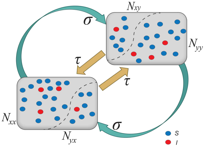
We first specify the mechanism of commuting mobility to transfer individuals between subpopulations. Consider two coupled subpopulations, x, y, each of which has a population size of the residents  . They act as the reaction places where the contagion process occurs. The model proceeds at discrete time steps, with the unit interval as one hour. Individuals leave their original resident subpopulation x(y) to visit the neighboring ‘destination’ subpopulation y(x) with a per capita diffusion rate σxy(σyx) at each time step, and the displaced commuters will return to their residence x(y) with a per capita return rate τx(τy) per unit time. For simplicity, we assume the detailed balance as: σxy = σyx = σ, τx = τy = τ, and Figure 1 illustrates the commuting process.
Figure 1. Schematic illustration of the commuting process between two subpopulations x, y.
The cyan and orange arrows indicate the back and forth commuting flows.
According to Refs. 26, 52, the residents of each subpopulation can be partitioned into two subgroups based on the locations where they actually are at time t (see Figure 1). Define Nxx(t)(Nyy(t)) the subgroup size of the individuals staying in their original resident subpopulation x(y) at time t, and Nxy(t)(Nyx(t)) the subgroup size of the individuals from subpopulation x(y) presenting in the subpopulation y(x) at time t. Therefore, the population size of the residents of each subpopulation is  ,
,  . We use the mean-field approximation to describe the commuting process with a set of rate equations governing the evolution of population dynamics26,52, which are discussed in Supplementary Information, and we have the following equilibria:
 |
with the condition σ−1 ≫ τ−1, i.e., averagely, individuals will remain at their residence most of the time, which mimics that in reality only a small fraction of residents leave to travel. This condition facilitates the analysis by considering that per unit time each subpopulation x(y) has an effective number of residents  interacting with the individuals in subgroup Nyy(Nxx).
The contagion process takes place inside each subpopulation, which is composed of the infection dynamics and the contact dynamics here. For the infection dynamics, we consider the standard SIS compartment model. At time t, each individual falls in one of the disease compartments: susceptible or infectious. The population size, e.g., Nxx(t) (Nyx(t)), can be divided into Sxx(t)(Syx(t)), Ixx(t)(Iyx(t)), which is the number of susceptible and infectious individuals in each subgroup, respectively. At each time step, if a susceptible individual contacts an infectious one, he may acquire the infection with transmission rate β. An infectious individual recovers and becomes susceptible again with rate ν per unit time.
We now specify the contact dynamics in more detail. In the case of the type-I (destination-driven) contact scenario, we assume that per unit time each individual staying in subpopulation x(y) has the same characteristic contact rate cx(cy). Figure S1(a) in Supporting Information illustrates this case. In the unit interval, the infection probability, λ, for a susceptible individual is determined by all his contacts with the infectious ones. Therefore, the force of infection for any susceptible in subgroup Nxy or Nyy at time t is
where λy(t) characterizes the probability that a random contact with any individual staying in subpopulation y will lead to the infection at time t. Similarly, the force of infection for any susceptible in subgroup Nyx or Nxx at time t is
With the mean-field approximation, the contagion process in each subgroup under the type-I scenario can be delineated by a set of rate equations (see Eqs.(S5)–(S8) in Supplementary Information).
We next extend to the type-II (origin-driven) contact scenario. Per unit time, an individual from subpopulation x(y) has the characteristic rate of contacts,  , which means that on average he encounters with
  persons, no matter where he is (see Figure S1(b) for the illustration). With the mean-field approximation, the contagion process in each subgroup under the type-II scenario can also be described by the formalism of rate equations as Eqs. (S5)–(S8), except the expressions of the force of infection. The force of infection for any susceptible staying in subgroup Nxy at time t obeys the following relation
where  denotes the probability that a random contact with any individual staying in subpopulation y will lead to the infection. It is worth emphasizing that to normalize the fraction of contacts of the infectious ones in each subpopulation, the denominator of Eq.(4) should be the total number of contacts of the population instead of the total number of individuals staying in the subpopulation. Similarly, the force of infection for a susceptible presenting in other subgroups at time t are as follows:
Besides, we consider a baseline scenario that the contact rate in each subpopulation is equal to 〈c〉 = (cx + cy)/2, which corresponds to the traditional situation that the contact pattern in all subpopulations is uniform. In this case, the epidemic threshold is captured by the basic reproductive number,  , which identifies the expected number of secondary infections produced by an infected individual during his infectious period within the entire susceptible population1,2,3,41,58. If
  , the whole system remains at the disease-free state.
Analysis
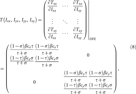
With embedding the aforementioned contact features, the epidemic threshold can be characterized by an extended version of the basic reproductive number  2,41,58. We first build the next generation matrix (NGM) TΣ−1 from the rate equations (S5)–(S8) at the disease-free equilibrium (DFE). Under the type-I contact scenario, the transmission matrix T is defined as
 |
while under the type-II contact scenario, the transmission matrix T is
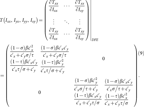 |
In the above two matrices, each entry Tij(i, j ∈ (x, y)) represents the rate of generating new infections in subgroup Nij. In these two scenarios, the transition matrix Σ is
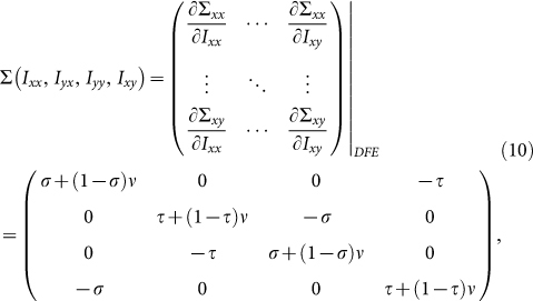 |
where  denotes the rate of transferring infectious individuals into subgroup Nij, while
  denotes the rate of transferring infectious people out of Nij. The recovery of infective individuals also decreases the number of infectious ones, and thus is included in
  . The matrices T and Σ are obtained at the disease-free equilibrium. The global version of the basic reproductive number is calculated by the spectral radius of the NGM41,58:
Since the explicit expression of the threshold is unavailable, we present the numerical results in the following.
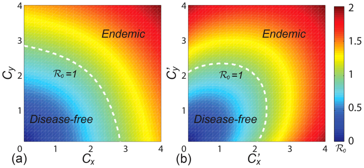
Figure 2 presents the  phase diagrams of the global
  . As the empirical evidence tells that the commuting takes place at the time scale τ−1 ~ 1/3 day36, we choose the return rate τ = 0.125/hour. For the diffusion rate, we first set a large value σ = 0.042/hour, which implies that the time scale of diffusion is 1 day. We set other parameters of the disease as: ν = 0.042/hour (a short duration for the mean infectious period), and β = 0.021/hour. Note that fixing the disease parameters as other values does not change the main results of this paper. The white dashed line in each panel indicates the parametric values corresponding to the threshold
  . The evident difference of the thresholds between the two heterogeneous contact scenarios shows that the type-II contact manner may induce the disease outbreak at much lower contact rates. This is due to the fact that the commuting process facilitates each subpopulation x(y) to share an effective number of individuals
  into the neighboring subpopulation y(x). As the displaced commuters will closely interact with local residents, individuals with distinct contact rates have the opportunity to directly encounter in each subpopulation under the type-II scenario.
Figure 2. The  phase diagrams of the global
  .
.
(a) presents the type-I contact scenario. (b) presents the type-II contact scenario. The white dashed curve in each panel illustrates the threshold of contact rates. We fix τ = 0.125/hour, σ = 0.042/hour, β = 0.021/hour, ν = 0.042/hour.
As shown in Figure 2(a), one can find a monotonic mode for the variance of global  under the type-I scenario, which positively correlates to the increase of contact rates cx and cy. The results are more complex under the type-II scenario (see Figure 2(b)), because the values of global
  at the upper-left and lower-right corners of the phase diagram are also very large. The variance of
  does not show a monotonic mode when
  or
or  is large (> 2.34) in the case of type-II scenario. For instance, when
  ,
,  gradually decreases until reaches the bottom, then monotonically grows with the increase of
  .
.
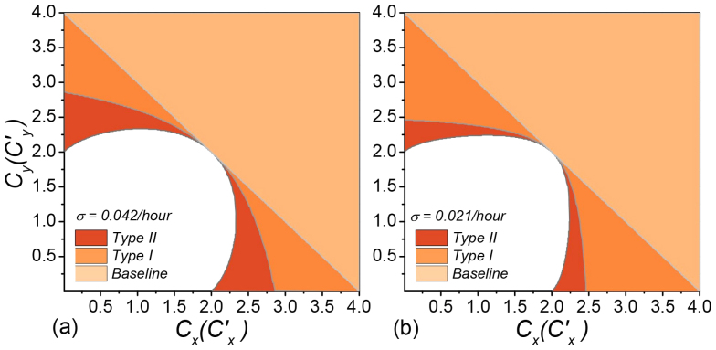
We further compare the parametric regions of the endemic phases among the baseline, type-I, and type-II scenarios with the aforementioned parameters, as shown in Figure 3(a). The upper triangular light orange area corresponds to the baseline with  . The parametric space of the type-I or type-II scenario with the global
  is much broader than that of the baseline case. Therefore, the inclusion of both two location-specific heterogeneous contact patterns favors the epidemic outbreak. It is also of interest to inspect the effect of a smaller diffusion rate σ on the threshold, since reducing σ weakens the coupling between subpopulations. Figure 3(b) compares the parametric regions pertaining to the endemic phases among the baseline, type-I, and type-II scenarios with σ = 0.021/hour, which yields the same results.
Figure 3. Comparison of the parametric space pertaining to the endemic phases among the baseline, type-I, and type-II contact scenarios.
τ = 0.125, ν = 0.042, β = 0.021/hour, and σ = 0.042/hour in (a) and σ = 0.021/hour in (b).
Simulations
To verify the above analysis, we use the dynamic Monte Carlo method to simulate the epidemic evolution. We focus on inspecting the parametric space of contact rates. With each set of parameters, we monitor the dynamical evolution of epidemic spreading in each subpopulation, and record the disease prevalence (the fraction of infectious individuals) in subpopulation x(y), Ix(t)/Nx(Iy(t)/Ny), where Nx = Nxx(t) + Nyx(t) (Ny = Nyy(t) + Nxy(t)). Due to the presence of stochasticity, each independent Monte Carlo simulation generates a random realization of the dynamic process. We perform 103 random Monte Carlo simulations for each set of parameters.
Initially, each subpopulation has 105 individuals, i.e., Nxx(0) = Nyy(0) = 105, Nxy(0) = Nyx(0) = 0. We fix the return rate τ = 0.125/hour and the diffusion rate σ = 0.042/hour to stress the coupling effect. Figure S2 presents the time series of population evolution in each subgroup. As analyzed in Supplementary Information, the population size of each subgroup quickly reaches to the equilibrium:  ,
,  . Then we simulate the contagion process with a variety of typical sets of contact rates, fixing the transmission parameters β = 0.021, ν = 0.042/hour. The status of each individual is updated in parallel per unit time. The mobility and disease parameters are directly converted into the probabilities with the unitary time scale of one hour. The algorithm details of the simulation see the section of Methods.
We start the contagion process by introducing the seeds of infectious individuals into a given subgroup. For simplicity, the case of multiple introductions is not considered here, i.e., the seeds are only introduced into one subgroup. The contagion process begins with Ixx(0) = 50,  , Iyx(0) = Iyy(0) = Ixy(0) = 0. By fixing the transmission parameters β = 0.021, ν = 0.042, we mainly study the stationary prevalence (SP)
  ,
,  with different parameters (SP reflects the average fraction of infectious individuals in each subpopulation at the equilibrium). To obtain each data point, we perform 103 Monte Carlo random experiments, each of which is simulated with 104 time steps. We define an outbreak run as the realization that the number of infectious individuals at the equilibrium is larger than 50. The stationary prevalence is calculated by averaging over all the outbreak realizations. We first record the mean value of the number of infectious individuals in each subpopulation over the last 10% time steps of each outbreak simulation, then average them to obtain the stationary prevalence. If there does not exist an outbreak run,
  .
.
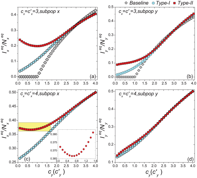
In Figs. 4–5, we compare the phase diagrams of the stationary prevalence  ,
,  among the baseline, type-I, and type-II contact scenarios with several typical
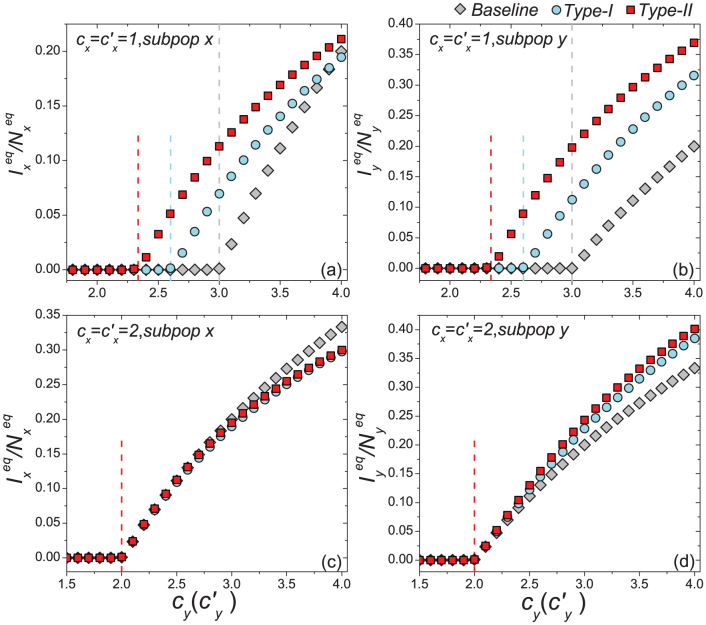
  . Figures 4(a)–(b) show the variance of
  ,
,  as
as  gradually increases, fixing
  . The thresholds of contact rate
  , which separate the transition from the disease-free phase to the endemic phase, of both the type-I and type-II scenarios are much smaller than that of the baseline case, while the threshold of type-II scenario is the smallest. We also observe the well agreement between the simulations and analysis, as illustrated by the colored dashed lines in each panel. In the endemic phase, we find a counterintuitive phenomenon that, with the same parameters, the stationary prevalence
  ,
,  of the type-II scenario are larger than those of the type-I scenario. In subpopulation x, the larger
  of the type-II scenario might relate to the introduction of individuals with a higher contact rate. However, in subpopulation y, it seems a little unexpected that the type-II scenario leads to a larger
  , because under the type-II scenario the displaced commuters from subpopulation x to y have a smaller contact rate when the global
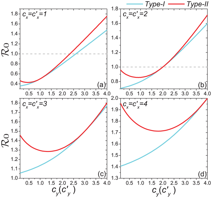
  . In Figure 6(a), we compare the phase diagrams of global
  between the type-I and type-II contact scenarios, fixing
  . When
  , with the same contact rate
  , the global
  of the type-II scenario is evidently larger than that of the type-I scenario, which means that with the same parameters, the prevalence is more serious in the former one. Since we assume that the individual contact rate keeps unchanged in the case of type-II scenario, this outcome may be due to the fact that individuals staying in subgroup Nyy increase their “within self-subgroup” contacts compared with those of the type-I scenario.
Figure 4. Comparison of the phase diagrams of  ,
,  among the baseline, type-I, and type-II scenarios.
(a)(b) show the variance of  and
and  as
as  gradually increases, fixing
  (c)(d) show the variance of
  and
and  as
as  gradually increases, fixing
  . The error bar is not shown since the standard deviation is much smaller (less than 10−1 of the mean value). The vertical colored dashed lines illustrate the theoretical prediction of the threshold of
  .
.
Figure 5. Comparison of the phase diagrams of  ,
,  among the baseline, type-I, and type-II contact scenarios.
(a)(b) show the variance of  and
and  as
as  gradually increases, fixing
  . (c)(d) show the variance of
  and
and  as
as  gradually increases, fixing
  . The inset in (c) shows the enlargement of the yellow area in that panel. The error bar is not shown since the standard deviation is much smaller.
Figure 6. Comparison of the phase diagrams of global  between the type-I and type-II contact scenarios.
Each panel shows the variance of global  as
as  gradually increases, with
  in (a),
  in (b),
  in (c),
  in (d). The horizontal gray dashed lines in the upper two panels illustrate the threshold value
  .
.
Figures 4(c)–(d) present the variance of stationary prevalence  ,
,  as
as  gradually increases, fixing
  . In this case, the thresholds of contact rate
  for the baseline, type-I, and type-II scenarios overlap at
  , which is also supported by Eq.(11) as indicated by the red dashed line in each panel. In the endemic phase of
  , the difference of stationary prevalence between the type-I and type-II processes is largely shrunk. Figure 6(b) compares the phase diagrams of global
  with fixing
  . In the case of a large
  , the difference of
  becomes smaller than that of the former situation
  .
.
When we further increase  , e.g.,
  or
or  , the outcomes are more complex. Figures 5(a)–(b) show the variance of
  ,
,  as
as  gradually increases, fixing
  . In the baseline case, both the simulations and analysis agree that the threshold of contact rate decreases to cy = 1. The heterogeneous contact scenarios yield that the threshold of
  vanishes. Figures 5(c)–(d) present the variance of
  ,
,  in dependence on
  , fixing
  . Since the threshold of contact rate of the baseline also vanishes, the baseline results are not included in Figures 5(c)(d). The analytical results of global
  (see Figures 6(c)(d)) indicate that the disease-free phase is eliminated, no matter how small
  is.
is.
Moreover, under the type-I process, both  and
and  monotonically increase with the augment of cy, as shown in Figure 5. Under the type-II process, it is evident that
  also monotonically increases with the growth of
  , while
  first gradually decreases, after reaching the bottom it begins to monotonically grow with the increase of
  . The variance of global
  under the type-II scenario also experiences a valley as
  gradually increases (see Figure 6). To explain this untrivial phenomenon, we observe the stationary prevalence of each subgroup in detail. As an example, we present the results of
  in Figure 7. It is clear that
  and
and  monotonically increase with the increment of
  , whereas the variances of
  and
and  are nonmonotonic. In subpopulation x, the probability of an individual of subgroup Nxx to involve in a contact is
  , while the probability of an individual of subgroup Nyx to involve in a contact is
  . With the increase of
  , the individuals in subgroup Nxx will reduce their ‘within self-subgroup’ contacts. As
  initially grows from 0.1, the net loss of infectious individuals in subgroup Nxx suppresses the gain obtained from subgroup Nyx, because
  . In this stage, the presence of commuters from subpopulation y mitigates the epidemic situation in subpopulation x, and their influence will be enhanced with the increment of
  . Thus one can observe the counterintuitive drop of
  . In subpopulation y, with the increase of
  , the net increase of infectious individuals in subgroup Nyy can compensate the loss of subgroup Nxy, because
  . Therefore,
  keeps on increasing as shown in Figure 5(b). As subpopulations x, y are coupled together, increasing
  will eventually cease the decline of
  . After hitting the bottom,
  positively correlates with the increase of
  .
.
Figure 7. Variance of the stationary prevalence of infectious individuals in subgroups Nxx, Nxy (a), Nyy, Nyx (b) as  gradually increases, under the type-II scenario.
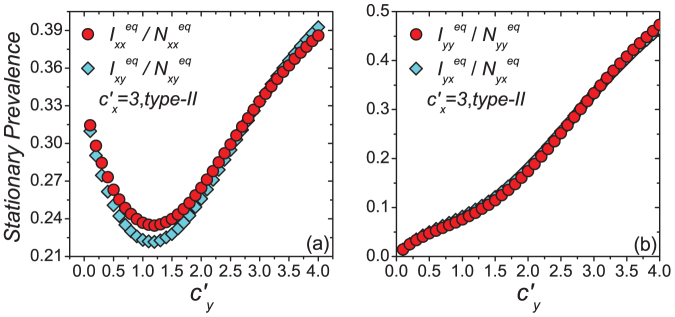
We fix  .
.
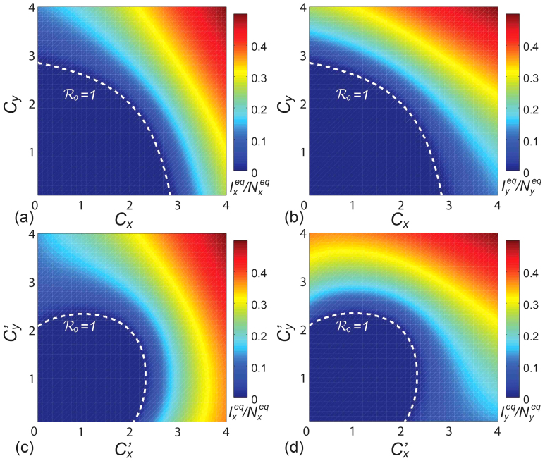
As a brief summary, we present the  phase diagrams of the stationary prevalence
  and
and  under the type-I and type-II scenarios, and give a holistic view about the impact of different contact patterns on the spatial transmission between populations. Figures 8(a)–(b) plot the cx−cy phase diagrams of
  and
and  under the type-I scenario, respectively. One can clearly observe the monotonic increase of
  and
and  with the increment of cx and cy. The white dashed line in each panel illustrates the threshold of contact rates leading to the global
  (calculated by the NGM method), which successfully separates the endemic phase from the disease-free phase. Similarly, Figures 8(c)–(d) show the
  phase diagrams of
  and
and  under the type-II scenario, respectively. The parametric space corresponding to the endemic phase under the type-II scenario is broader than that of the type-I scenario. When
  or
or  , the stationary prevalence
  and
and  does not always monotonically increase with the augment of
  ,
,  . In this case, the increment of contact rates will reduce the disease prevalence
  or
or  in some parametric regimes.
Figure 8. The  phase diagrams of
  ,
,  .
.
(a)(b) show the type-I scenario. (c)(d) show the type-II scenario. The white dashed curve in each panel illustrates the threshold of contact rates leading to the global  .
.
Discussion
With the evidence of location-related factors in reality, we have introduced two categories of location-specific contact patterns in a phenomenological structured populations model based on the commuting and contagion processes. Through theoretical analysis and extensive computational simulations, we have shown that these heterogeneous contact scenarios favor the disease outbreaks and evidently decrease the epidemic threshold of the entire system. This finding is robust against the changing of system parameters. More specifically, under the destination-driven scenario, the variance of disease prevalence exhibits the monotonic dependence of contact rates, while under the origin-driven scenario the increment of contact rates unexpectedly reduces the disease prevalence in some parametric regimes. Compared to the traditional framework, where the contact pattern in all subpopulations is uniform, the models presented in this paper demonstrate that the inclusion of these extra factors raises the risk of infection, mainly due to the presence of couplings between populations. Therefore, the interventions to limit the mobility flows, e.g., entry screening, and travel restriction, may benefit to control the disease invasion. To better understand the impact of human contact behaviors on the spatial transmission of infectious disease, more efforts are deserved to deal with more heterogeneous networking populations in further studies.
Methods
Algorithm details
The contagion and commuting processes at each time step proceed as follows:
(i) Contagion process. For the type-I scenario, the probability of a susceptible staying in subpopulation x to acquire the infection by each of his contacts at time t is λx(t) = β(Ixx(t) + Iyx(t))/(Nxx(t) + Nyx(t)). Therefore, the force of infection for each susceptible staying in subgroup Nxx or Nyx is λxx(t) = λyx(t) = cxλx(t). Similarly, the force of infection for each susceptible staying in subgroup Nyy or Nxy at time t is λyy(t) = λxy(t) = cyλy(t). At this time step, the number of new infections in subgroup Nxy is generated from a binomial distribution with probability λxy(t) and the number of trials Sxy(t). The number of new infections in other subgroups is generated in the same way. At the same time, any infectious individual recovers and becomes susceptible again with rate ν. The number of recovered individuals in each subgroup is generated from a binomial distribution with probability ν and the number of trials defined by the number of infectious individuals in that subgroup.
For the type-II scenario, each resident of subpopulation x(y) contacts with  other individuals in his current location per unit time. At time t, the probability of a susceptible presenting in subpopulation y to acquire the infection by each of his contacts is
  . Thus the force of infection of each susceptible in subgroup Nxy is
  , while the force of infection of each susceptible in subgroup Nyy is
  . The forces of infection of susceptible individuals in other subgroups are obtained similarly. At this time step, the number of new infections in subgroup Nxy is generated from a binomial distribution with probability
  and the number of trials Sxy(t). The number of new infections in other subgroups is generated in the same way. At each time step, the number of recovered individuals in each subgroup is generated from a binomial distribution with probability ν and the number of trials defined by the number of infectious individuals in that subgroup.
(ii) Commuting process. At each time step, after all individuals update the contagion dynamics, the simulation moves to their commuting process. The number of susceptible travelers departing from their resident subpopulation x(y) per unit time is generated from a binomial distribution with probability σ and the number of trials Sxx(t)(Syy(t)). The number of susceptible commuters returning to their residence x(y) per unit time is also generated from a binomial distribution with probability τ and the number of trails Sxy(t)(Syx(t)). The number of infectious individuals leaving from or returning to their residence is acquired in the same way.
Author Contributions
L.W., Z.W. and X.L. planned the study; L.W., Y.Z. and Z.W. performed the experiments, analyzed the data, and prepared the figures; L.W., Z.W. and X.L. wrote the paper.
Supplementary Material
Supplementary Information
Acknowledgments
This work was partly supported by National Key Basic Research and Development Program (No.2010CB731403), the National Natural Science Foundation(No. 61273223), and the Research Fund for the Doctoral Program of Higher Education (No. 20120071110029) of China. LW also acknowledges the partial support by Fudan University Excellent Doctoral Research Program (985 Project).
References
- Anderson R. M. & May R. M. Infectious Diseases of Humans: Dynamics and Control (Oxford University Press, Oxford, UK, 1991). [Google Scholar]
- Diekmann O. & Heesterbeek J. A. P. Mathematical Epidemiology of Infectious Diseases: Model Building, Analysis and Interpretation (John Wiley & Sons, New York, 2000). [Google Scholar]
- Keeling M. J. & Rohani P. Modeling Infectious Diseases in Humans and Animals (Princeton University Press, Princeton and Oxford, 2008). [Google Scholar]
- Boccaletti S., Latora V., Moreno Y., Chavez M. & Hwang D. U. Complex networks: Structure and dynamics. Phys. Rep. 424, 175–308 (2006). [Google Scholar]
- Newman M. E. J. Networks: An Introduction (Oxford University Press, New York, 2010). [Google Scholar]
- Perc M. & Szolnoki A. Coevolutionary games – A mini review. BioSystems 99, 109–125 (2010). [DOI] [PubMed] [Google Scholar]
- Csermely P. Weak Links: The Universal Key to the Stability of Networks and Complex Systems (Springer-Verlag, Berlin, Heidelberg, 2006). [Google Scholar]
- Vespignani A. Modelling dynamical processes in complex socio-technical systems. Nat. Phys. 8, 32–39 (2012). [Google Scholar]
- Perc M., Gómez-Gardeñnes J., Szolnoki A., Floría L. M. & Moreno Y. Evolutionary dynamics of group interactions on structured populations: A review. J. R. Soc. Interface 10, 20120997 (2013). [DOI] [PMC free article] [PubMed] [Google Scholar]
- Meyers L. A., Pourbohloul B., Newman M. E. J., Skowronski D. M. & Brunham R. C. Network theory and SARS: Predicting outbreak diversity. J. Theor. Biol. 232, 71–81 (2005). [DOI] [PMC free article] [PubMed] [Google Scholar]
- Li X. & Wang X. F. Controlling the spreading in small-world evolving networks: Stability, oscillation, and topology. IEEE Trans. Automat. Control 51, 534–540 (2006). [Google Scholar]
- Zhou T., Liu J. G., Bai W. J., Chen G. R. & Wang B.-H. Behaviors of susceptible-infected epidemics on scale-free networks with identical infectivity. Phys. Rev. E 74, 056109 (2006). [DOI] [PubMed] [Google Scholar]
- Gómez-Gardeñes J., Latora V., Moreno Y. & Profumo E. Spreading of sexually transmitted diseases in heterosexual populations. Proc. Natl. Acad. Sci. USA 105, 1399–1404 (2008). [DOI] [PMC free article] [PubMed] [Google Scholar]
- Meloni S., Arenas A. & Moreno Y. Traffic-driven epidemic spreading in finite-size scale-free networks. Proc. Natl. Acad. Sci. USA 106, 16897–16902 (2009). [DOI] [PMC free article] [PubMed] [Google Scholar]
- Parshani R., Carmi S. & Havlin S. Epidemic threshold for the susceptible-infectious-susceptible model on random networks. Phys. Rev. Lett. 104, 258701 (2010). [DOI] [PubMed] [Google Scholar]
- Castellano C. & Pastor-Satorras R. Thresholds for epidemic spreading in networks. Phys. Rev. Lett. 105, 218701 (2010). [DOI] [PubMed] [Google Scholar]
- Rvachev L. A. & Longini I. M. Jr A mathematical model for the global spread of influenza. Math. Biosci. 75, 3–22 (1985). [Google Scholar]
- Watts D., Muhamad R., Medina D. C. & Dodds P. S. Multiscale, resurgent epidemics in a hierarchical metapopulation model. Proc. Natl. Acad. Sci. USA 102, 11157–11162 (2005). [DOI] [PMC free article] [PubMed] [Google Scholar]
- Viboud C. et al. Synchrony, waves, and spatial hierarchies in the spread of influenza. Science 312, 447–451 (2006). [DOI] [PubMed] [Google Scholar]
- Colizza V., Pastor-Satorras R. & Vespignani A. Reaction-diffusion processes and metapopulation models in heterogeneous networks. Nat. Phys. 3, 276–282 (2007). [Google Scholar]
- Tang M., Liu Z. H. & Li B. W. Epidemic spreading by objective traveling. Europhys. Lett. 87, 18005 (2009). [Google Scholar]
- Wang L., Li X., Zhang Y. Q., Zhang Y. & Zhang K. Evolution of scaling emergence in large-scale spatial epidemic spreading. PLoS One 6, e21197 (2011). [DOI] [PMC free article] [PubMed] [Google Scholar]
- Meloni S. et al. Modeling human mobility responses to the large-scale spreading of infectious diseases. Sci. Rep. 1, 62 (2011). [DOI] [PMC free article] [PubMed] [Google Scholar]
- Wang B., Cao L., Suzuki H. & Aihara K. Safety-information-driven human mobility patterns with metapopulation epidemic dynamics. Sci. Rep. 2, 887 (2012). [DOI] [PMC free article] [PubMed] [Google Scholar]
- Belik V., Geisel T. & Brockmann D. Natural human mobility patterns and spatial spread of infectious diseases. Phys. Rev. X 1, 011001 (2011). [Google Scholar]
- Balcan D. & Vespignani A. Invasion threshold in structured populations with recurrent mobility patterns. J. Theor. Biol. 293, 87–100 (2012). [DOI] [PMC free article] [PubMed] [Google Scholar]
- Hufnagel L., Brockmann D. & Geisel T. Forecast and control of epidemics in a globalized world. Proc. Natl. Acad. Sci. USA 101, 15124–15129 (2004). [DOI] [PMC free article] [PubMed] [Google Scholar]
- Hollingsworth T. D., Ferguson N. M. & Anderson R. M. Will travel restrictions control the international spread of pandemic influenza? Nat. Med. 12, 497–499 (2006). [DOI] [PubMed] [Google Scholar]
- Epstein J. M. et al. Controlling pandemic flu: The value of international air travel restrictions. PLoS One 2, e401 (2007). [DOI] [PMC free article] [PubMed] [Google Scholar]
- Cooper B. S., Pitman R. J., Edmunds W. J. & Gay N. J. Delaying the international spread of pandemic influenza. PLoS Med. 3, e212 (2006). [DOI] [PMC free article] [PubMed] [Google Scholar]
- Khan K. et al. Spread of a novel influenza A (H1N1) virus via global airline transportation. N. Engl. J. Med. 361, 212–214 (2009). [DOI] [PubMed] [Google Scholar]
- Kenah E., Chao D. L., Matrajt L., Elizabeth Halloran M. & Longini I. M. Jr The global transmission and control of influenza. PLoS One 6, e19515 (2011). [DOI] [PMC free article] [PubMed] [Google Scholar]
- Bajardi P. et al. Human mobility networks, travel restrictions, and the global spread of 2009 H1N1 pandemic. PLoS One 6, e16591 (2011). [DOI] [PMC free article] [PubMed] [Google Scholar]
- Wang L., Zhang Y., Huang T. Y. & Li X. Estimating the value of containment strategies in delaying the arrival time of an influenza pandemic: A case study of travel restriction and patient isolation. Phys. Rev. E 86, 032901 (2012). [DOI] [PubMed] [Google Scholar]
- González M. C., Hidalgo C. A. & Barabási A. L. Understanding individual human mobility patterns. Nature 453, 779–782 (2008). [DOI] [PubMed] [Google Scholar]
- Balcan D. et al. Multiscale mobility networks and the spatial spreading of infectious diseases. Proc. Natl. Acad. Sci. USA 106, 21484–21489 (2009). [DOI] [PMC free article] [PubMed] [Google Scholar]
- Song C. M., Qu Z. H., Blumm N. & Barabási A.-L. Limits of predictability in human mobility. Science 327, 1018–1021 (2010). [DOI] [PubMed] [Google Scholar]
- Keeling M. J., Danon L., Vernon M. C. & House T. A. Individual identity and movement networks for disease metapopulations. Proc. Natl. Acad. Sci. USA 107, 8866–8870 (2010). [DOI] [PMC free article] [PubMed] [Google Scholar]
- Simini F., González M. C., Maritan A. & Barabási A. L. A universal model for mobility and migration patterns. Nature 484, 96–100 (2012). [DOI] [PubMed] [Google Scholar]
- Mossong J. et al. Social contacts and mixing patterns relevant to the spread of infectious diseases. PLoS Med. 5, e74 (2008). [DOI] [PMC free article] [PubMed] [Google Scholar]
- Cao L., Li X., Wang B. & Aihara K. Rendezvous effects in the diffusion process on bipartite metapopulation networks. Phys. Rev. E 84, 041936 (2011). [DOI] [PubMed] [Google Scholar]
- Fumanelli L. et al. Inferring the structure of social contacts from demographic data in the analysis of infectious diseases spread. Plos Comput. Biol. 8, e1002673 (2012). [DOI] [PMC free article] [PubMed] [Google Scholar]
- Eagle N., Pentland A. & Lazer D. Inferring friendship network structure by using mobile phone data. Proc. Natl. Acad. Sci. USA 106, 15274–15278 (2009). [DOI] [PMC free article] [PubMed] [Google Scholar]
- Cattuto C. et al. Dynamics of person-to-person interactions from distributed RFID sensor networks. PLoS One 5, e11596 (2010). [DOI] [PMC free article] [PubMed] [Google Scholar]
- Isella L. et al. What's in a crowd? Analysis of face-to-face behavioral networks. J. Theor. Biol. 271, 166–180 (2011). [DOI] [PubMed] [Google Scholar]
- Takaguchi T., Nakamura M., Sato N., Yano K. & Masuda N. Predictability of conversation partners. Phys. Rev. X 1, 011008 (2011). [Google Scholar]
- Salathé M. et al. A high-resolution human contact network for infectious disease transmission. Proc. Natl. Acad. Sci. USA 107, 22020–22025 (2010). [DOI] [PMC free article] [PubMed] [Google Scholar]
- Zhang Y., Wang L., Zhang Y. Q. & Li X. Towards a temporal network analysis of interactive WiFi users. Europhys. Lett. 98, 68002 (2012). [Google Scholar]
- Zhang Y. Q. & Li X. Characterizing large-scale population's indoor spatio-temporal interactive behaviors. Proc. ACM SIGKDD Int. Workshop on Urban Computing (UrbComp’12) 25–32 (2012). [Google Scholar]
- Lessler J. et al. Location-specific patterns of exposure to recent pre-pandemic strains of influenza A in southern China. Nat. Commun. 2, 423 (2011). [DOI] [PMC free article] [PubMed] [Google Scholar]
- Crighton E. J., Elliott S. J., Moineddin R., Kanaroglou P. & Upshur R. E. An exploratory spatial analysis of pneumonia and influenza hospitalizations in Ontario by age and gender. Epidemiol. Infect. 135, 253–261 (2007). [DOI] [PMC free article] [PubMed] [Google Scholar]
- Keeling M. J. & Rohani P. Estimating spatial coupling in epidemiological systems: a mechanistic approach. Ecol. Lett. 5, 20–29 (2002). [Google Scholar]
- Perc M. Sustainable institutionalized punishment requires elimination of second-order free-riders. Sci. Rep. 2, 344 (2012). [DOI] [PMC free article] [PubMed] [Google Scholar]
- Szolnoki A., Perc M. & Szabó G. Defense mechanisms of empathetic players in the spatial ultimatum game. Phys. Rev. Lett. 109, 078701 (2012). [DOI] [PubMed] [Google Scholar]
- Gracia-Lazaro C., Cuesta J. A., Sánchez A. & Moreno Y. Human behavior in Prisoner's Dilemma experiments suppresses network reciprocity. Sci. Rep. 2, 325 (2012). [DOI] [PMC free article] [PubMed] [Google Scholar]
- Wilson T. D., Houston C. E., Etling K. M. & Brekke N. A new look at anchoring effects: Basic anchoring and its antecedents. J. Exp. Psychol. 125, 387–402 (1996). [DOI] [PubMed] [Google Scholar]
- Furnham A. & Boo H. C. A literature review of the anchoring effect. Journal of Socio-Economics 40, 35–42 (2011). [Google Scholar]
- Heffernan J. M., Smith R. J. & Wahl L. M. Perspectives on the basic reproductive ratio. J. R. Soc. Interface 2, 281–293 (2005). [DOI] [PMC free article] [PubMed] [Google Scholar]
Associated Data
This section collects any data citations, data availability statements, or supplementary materials included in this article.
Supplementary Materials
Supplementary Information


