Between algorithm and model: different Molecular Surface definitions for the Poisson-Boltzmann based electrostatic characterization of biomolecules in solution

Abstract

The definition of a molecular surface which is physically sound and computationally efficient is a very interesting and long standing problem in the implicit solvent continuum modeling of biomolecular systems as well as in the molecular graphics field. In this work, two molecular surfaces are evaluated with respect to their suitability for electrostatic computation as alternatives to the widely used Connolly-Richards surface: the blobby surface, an implicit Gaussian atom centered surface, and the skin surface. As figures of merit, we considered surface differentiability and surface area continuity with respect to atom positions, and the agreement with explicit solvent simulations. Geometric analysis seems to privilege the skin to the blobby surface, and points to an unexpected relationship between the non connectedness of the surface, caused by interstices in the solute volume, and the surface area dependence on atomic centers. In order to assess the ability to reproduce explicit solvent results, specific software tools have been developed to enable the use of the skin surface in Poisson-Boltzmann calculations with the DelPhi solver. Results indicate that the skin and Connolly surfaces have a comparable performance from this last point of view.

1 Introduction

Biomolecular systems are composed of biological macromolecules, proteins and nucleic acids, and of a number of small organic molecules and electrolytes immersed in aqueous solution. The role of the solvent is sometimes crucial because of the effects it can have on the behavior of the biomolecules while performing their function. Therefore, both in the field of Computational Biological Chemistry and Molecular Visualization, Molecular Surfaces (MSs) play an instrumental role as the separation between the system one wants to monitor and the surrounding environment, whose effect cannot be neglected but that is usually not the focus of the analysis. In Computational Biological Chemistry, the so-called implicit solvent models provide an estimate of the average solvent effect, resulting in a huge computational saving, since the number of degrees of freedom of the solvent is usually much larger than that of the solute. Approaches based on the Poisson-Boltzmann Equation (PBE) [1] and the Generalized Born Approximation [2] are widely used to estimate the reaction of the media to the electric field generated by the partial charges on the solute. In particular, the Poisson-Boltzmann equation reads:

$$\nabla ·[\epsilon (\mathbf{r})\nabla \varphi (\mathbf{r})]=-\left[{\rho }^{\mathit{fixed}}+e\sum _{i=1}^{N_s}{C}_i(\infty )z_{i}exp\left(-\frac{{ez}_i}{k_{B}T}\varphi (\mathbf{r})\right)\right]$$ (1.1)

where e is the electron charge, C_i(∞) is the bulk concentration of the i-th ion type and z_i is its valence, k_B is the Boltzmann constant, T is the temperature, ρ^fixed represents the partial charge distribution and ϕ(r) the potential; ε(r) is the space varying dielectric constant, which is a direct consequence of the adopted surface definition. The solution of this equation is needed to acquire an accurate knowledge of the reaction field and it can also be used to derive the electrostatic forces exerted by the solvent on the solute, which are mostly located at the boundary between high and low dielectric regions, i.e. on the MS.

Traditionally, the simplest molecular models represent classical atoms as hard spheres whose radius, namely the van der Waals radius, indicates the largest distance at which an atom repels its neighbors. The union of these hard spheres is the so-called van der Waals volume and the resulting enclosing surface is termed the van der Waals surface (VDWS). In a real solvent, the solvent molecules have a finite size and small invaginations are not accessible, at least in a static scenario. To account for this fact, other surfaces were identified, in particular the Solvent Accessible Surface, which is the locus of the centers of a spherical probe that rolls over the molecular system. Geometrically, it coincides with the VDWS of the system where each VDW radius is increased by the size of the radius of the probe. In case of aqueous solution, a probe having the average water molecule radius of 1.4Å is considered. A subsequent development consisted in the definition of the Solvent Excluded Surface (SES), often identified with the Molecular Surface; it separates the volume accessible to a finite size solvent probe from the inaccessible one. This definition, based on a hard sphere model of both the solute and the solvent, was suggested by Lee and Richards [3] and an algorithm for its computation was provided by Connolly [4]. This approach became so widespread that the above described surface is often called Connolly surface, although Connolly algorithm is not the only one developed to this purpose [5] [6] [7].

The definition of the best MS model is a complex problem and the requirements it should satisfy are slightly different for the various context of use; for instance, for real-time visualization the emphasis is on speed, while in computational physics, the robustness, accuracy and interpretability of the simulation results are crucial aspects. In this work, we discuss the possibility that MS definitions originated in Computer Graphics and Applied Mathematics fields for visualization purposes can valuably contribute to applications in Physics and Biochemistry. We mainly focus on the so-called skin and blobby surfaces, and describe their suitability for the estimation of the electrostatic reaction field energy of biomolecular systems. To our knowledge, such analysis has not been done before and we believe it gives interesting insights in these alternative MS models. Lee and Richards’ MS is kept as a reference model and several figures of merit are adopted in this study; one of them is regularity, expressed in terms of: (i) the presence of regions where the normal vector is not defined; (ii) the continuous dependence of surface area on the position of the solute atomic centers; (iii) the generation of spurious high dielectric interstices in the solute region. Another important aspect is the agreement with energetic profiles generated by the Potential of Mean Force (PMF) in explicit solvent calculations (which can be considered as the ground truth), in line with the works of Masunov and Lazaridis [8] and Swanson, Mongan and McCammon [9]. In this work, we specialize our findings to the effects that might apply to the approach adopted by the DelPhi PBE solver [10], which maps the system on a grid where the equation is discretized and then iteratively solved. To this aim, we coupled different surface definitions to DelPhi and compared the results. The paper is organized as follows: first, a brief overview on MSs is performed, which includes some critical aspects for their application. In the Methods section the skin and the blobby surfaces are detailed together with the procedures used to make their assessment. In Section 4 the results of the analysis with respect to regularity and agreement with the PMF results are given. Finally, conclusions are drawn and a few comments on computational costs are given.

2 A brief survey on Molecular Surfaces

In this Section, alternative MS definitions are reported as well as some of the limitations that have been ascribed to the Lee and Richards’ MS and that hinder, for instance, its use in molecular dynamics applications.

2.1 From molecular visualization to implicit solvent models

For visualization purposes the most frequently adopted molecular surfaces are the VDWS and the SES [4]. Recently, both scientists in Computational Biological Chemistry and Computer Graphics developed different algorithms based on the Connolly method to derive the Lee and Richards surface. Besides the original Connolly algorithm [4], we would like to mention the Euclidean distance transform [11], Sanner MSMS package [5], the Contour-Build-up algorithm [7], the Level Set Method [12], the discretization with curved elements [13] and the method employed in the DelPhi PBE solver [6]. In the Computer Graphics community, algorithms were also developed for the classical Connolly surface: a NURBS based method [14], alpha shapes [15] and beta shapes [16].

Alternative MS definitions have also been suggested, see for instance Lu and Luo in [17] and in [18] among the others. The minimal molecular surface [19] is an elegant formalization of the MS problem: the resulting surface is implicit and can be triangulated via a standard meshing algorithm such as the “marching cubes” [20]. A completely different approach has been pursued in [21] and in [22], where the abrupt transition from high to low dielectric regions is abandoned in favor of a smooth spatial variation of the dielectric. This choice improves the convergence of the numerical PBE solvers but it does not resolve all of the remaining problems affecting the surface, while it pays the price of a higher complexity due to the fact that the polarization charge, which represents the dielectric reaction, is spread over a volumetric shell rather than over a surface.

Two alternative definitions of the molecular surface seem to be particularly promising: the blobby surface, an implicit surface based on the Gaussian atom centered idea adopted also in [22], and the skin surface, a more elaborated mathematical concept defined by Edelsbrunner [23]. The blobby surface, originally proposed in [24], but later enhanced in [25], is an implicit surface that is usually triangulated for visualization, while the skin can be either triangulated [26] [27] or Ray-Casted [28], [29], resulting in a very high quality rendering. We considered these surfaces for several reasons: chiefly, for their smoothness and because they are expected, due to their mathematical definition, to provide a surface area which is continuous with respect to both surface parameters and atom positions. Additionally, the blobby surface is interesting because it has a simple mathematical definition and it is inherently computationally parallel; in light of this fact, it has been implemented for instance in GAMER, a module of the APBS Poisson-Boltzmann solver [30] and parallelized by the Authors on a General Processing Unit (GPU) architecture [31]. With respect to the blobby, the skin surface is less intuitive in its geometric definition, but, similarly to the Connolly one, all of its patches can be analytically defined. This aspect well suits the DelPhi philosophy where the analytical nature of the MS is exploited as much as possible in order to reduce the finite grid size artifacts. Both blobby and skin surfaces are implicit; thus, one can consider using ray-tracing techniques for visualization, which involve a ray-surface intersection routine. Interestingly, the projection of a point over a surface, which is a primitive needed by DelPhi, also consists in a root finding problem as the intersection procedure and could benefit from a GPU implementation.

From the PBE solution standpoint, surface analyticity is not mandatory, since the most commonly used methods, namely Finite Differences, Boundary Elements and Finite Elements, rely on a discrete description of the boundary. However, one can observe that the analytical surface definition is used a posteriori by DelPhi [6], to improve the accuracy of the reaction field energy, and also in some Boundary Elements solvers [13].

2.2 On the regularity of Molecular Surfaces

Different applications have different requirements as far as regularity of the MS is concerned. Techniques using the positions and the normals of MS patches to calculate the electrostatic potential throughout the space, such as the Boundary Element Method for the solution of the PBE, are particularly sensitive to existence and continuity of the normal vector. The Connolly surface is a conceptually simple, physically sound and therefore widely accepted model also for PBE solution [10], [30], [32]; however, its definition suffers from some limitations, namely the possibility to have singularities and a discontinuous dependence of the surface area on the position of atom centers [17, 26, 29]. On the other side, it has already been pointed out that alternative MS definition based on atom centered functions may create unphysical high dielectric cavities that affect the estimation of the energy of the system [9]. In the following, these typical drawbacks are discussed also with respect to a possible use in the DelPhi solver.

2.2.1 Irregularity induced by self-intersections

Critical molecular conformations can occur where the fictitious solvent probe rolls in a region that has already been visited; this leads to so-called self-intersections, as described by Bajaj et al. [33]. The resulting spurious surface patches can be removed, or even avoided, as done by Lindow et al. [29] and by the DelPhi code [6], respectively.

As shown in Figure 1, the result of this removal leads to cusps or more extended loci where the normal vector is undefined. When the surface is used in a volumetric grid based numerical solver, the presence of these singularities does not affect much the potential calculated at the lattice points. However, when, as in the case of the DelPhi code, the polarization charge located in grid cubes containing the singularities is projected onto the MS a slight misplacement might occur.

Figure 1.

Self-intersection induced singularities of the Lee and Richards molecular surface; projected points computed from DelPhi surface algorithm

2.2.2 Cavities and voids

The presence of cavities in proteins has been well documented and studied [34]. In the following, we will call “cavities” regions in a macromolecule that are big enough to contain one or more water molecules, while we will term “voids” the smaller interstices due to local atomic displacements. Cavities can become accessible regions if the probe radius is so small that the MS tends to coincide with the VDWS; they can in principle contain actual water molecules but it is arguable that they can be assigned the same high dielectric constant as it is done in the bulk of the solvent. Moreover, if we consider a dynamic situation, the creation of a passage between the cavity and the external solvent is not unlikely. If the surface of the cavity was not counted as a patch of the MS, there could happen a very large and abrupt jump in the MS area, which has a very clear physical counterpart. In this case, the definition of the MS is not very influential and a possible solution might consist, for example, in treating explicitly the solvent in the cavity, maybe exploiting the DelPhi feature that assigns different dielectric constants to different parts of the system [10].

Much more relevant is the MS definition if voids are considered; as a matter of fact, small empty spaces between atoms can occur both in a crystal structure and, even more likely, during the dynamics of a macromolecule. Depending on the MS definition, it is possible that a high dielectric is assigned to the interior of these interstices. This is the case, for instance, for MSs based on atom centered functions as it has been pointed by Swanson et al. [9], and leads to an unphysical overestimation of the reaction of the dielectric media. The problem arising when these voids are located in the very close proximity of the MS is even more subtle. In fact, during the dynamics, there can be atomic displacements that continuously give and deny these small interstices access to the external solvent. If the MS definition is such that voids are “filled” of low dielectric medium, as it is the case of the Connolly surface, this leads to a discontinuity of the surface area corresponding to this open/close effect, as shown in Figures 9 and 10. As observed for instance by Luo et al. [17] and in [18], this phenomenon leads to a such serious instability in force determination that undermines its use in Molecular Dynamics applications.

Figure 9.

Surface Opening for the Connolly, skin and blobby

Figure 10.

Surface Areas for the Connolly, skin and blobby vs position

2.2.3 Dynamical picture of superficial voids

PBE is often used to process structures coming either from experimental measurements, e.g. X-ray diffraction crystal structures, or from computational models, e.g. homology modeling predictions, Molecular Dynamics trajectory snapshots in a ‘fixed point’ evaluation, based on atomic centers and radii. However, biological macromolecules are not frozen structures, they constantly undergo thermal fluctuations; in order to get a deeper understanding of the effect of quasi-superficial voids we considered a very simplified system where three atoms are positioned exactly in the configuration where the external probe is about to “fall” into the interstice. We then added a white gaussian zero-mean perturbation to the atomic positions of our model. For each perturbed configuration, we built the Connolly surface and stored the in/out information on a very fine lattice. At the end, we obtained for each point of the lattice the frequency of being inside the MS. Results are shown in the first panel of Figure 2; dark red regions are always inside while intense blue regions are always in the solvent, light blue regions correspond to critical regions with intermediate occupancy. The obvious consideration resulting from this simple experiment is that a soft sphere model for both the solute and the solvent probe would probably help to face the problem. The already discussed approaches that smoothen the space variability of the dielectric constant [21], [22] have a similar spirit. Sticking to an in/out description, if in our model we select an iso-frequency contour, we get the results shown in the second panel of Figure 2, where we show the surface comprising all the points that fell inside the Connolly MS in more than 50% of the cases upon random fluctuations around the critical configuration. Incidentally, it is interesting to note that, despite it descends from the Connolly surface, this method produces a surface devoid of the self-intersection induced irregularities.

Figure 2.

Thermal motion grid for three atoms; 0.5 level set surface

3 Methods

3.1 Mathematical definition and algorithmic implementation of alternative Molecular Surfaces

3.1.1 The skin surface

The skin surface was formally defined in [23]. The salient features for which we evaluated this surface as a promising alternative to the Connolly surface are the following:

• It can be decomposed in a finite set of trimmed quadric surfaces.

• There exist fast combinatorial algorithms (Regular Delaunay triangulation/Additively Weighted Voronoi diagram) to build it.

• Pathological configurations leading to normal discontinuity are extremely limited.

• Its area is continuous with respect to atom positions and radii.

Operatively the skin surface can be built starting from a set of weighted points S:

$$S=\{p_i=({\mathbf{x}}_i,w_i),{\mathbf{x}}_i\in {ℝ}^3,i=1,\dots ,n_a\}$$ (3.1)

and a shrink factor s ∈ (0,1]. When representing a molecule, the points x_i are the atom centers, n_a is the number of atoms and w_i are the weights. The weights w_i are defined as:

$$w_i=\frac{r_i^2}{s}$$ (3.2)

where r_i is the i-th atomic radius.

Shortly, the basic concept of the skin surface is the mixed complex; it is composed by mixed cells ${\mu }_X^s$, which are solids that can be computed starting from the additively weighted Voronoi diagram or its geometrically dual Delaunay tethraedrization [23]. The mixed cell is defined as the the Minkowsky sum (indicated by “⊕” and ruled by s) of a Voronoi cell with its corresponding Delaunay cell:

$${\mu }_X^s=\{s·{\nu }_X\oplus (1-s)·{\delta }_X\}$$ (3.3)

The mixed complex partitions ℝ³ in convex non overlapping polyedra and for s =0 and s = 1 it coincides with the Delaunay Tetrahedrization and the Voronoi diagram, respectively. All patches are quadric surfaces, either hyperboloids or spheres; each surface is trimmed by its corresponding mixed cell. Figure 3 represents the mixed complex and the corresponding skin surface.

Figure 3.

Skin Surface and mixed complex (transparent) in 2D and 3D. In 3D a simple case where 8 equal atoms are put on the vertices of a cube. Surfaces of the following mixed complexes ${\mu }_{0,3}^s,{\mu }_{3,0}^s,{\mu }_{2,1}^s$, and ${\mu }_{1,2}^s$ are represented in red, green, yellow and magenta, respectively.

To visualize the skin surface there are at least three possibilities: developing an algorithm to mesh the skin surface as in [26], [35], [27], performing a point sampling of the surface or exploiting the analytical structure of the skin to use ray casting techniques for quadrics [28] [29] and possibly also GPU capabilities to speed up the calculations.

Computing the skin surface is more expensive than computing the Connolly one; this fact has been empirically shown in [29]. Indeed, computing the skin surface requires first to compute a regular Delaunay tetrahedrization whose computational cost is O(nlogn) where n is in this case the number of atoms. After this step, the mixed complex computation and patches computation are required. Finally, in order to solve the Poisson-Boltzmann equation, a representation compatible with the DelPhi solver is needed: this means creating a dielectric volumetric map and in computing the projection of boundary grid points on the surface; both these steps are time consuming. Thus, to get a representation of the skin suitable for a finite difference solver, not only the skin surface must be computed but also imported in the DelPhi representation. However even neglecting the importation step, the time needed to build the regular Delaunay tetrahedrization is longer than the time needed to compute the Connolly surface either with the contour build-up algorithm as in [29] or using the algorithm currently implemented in DelPhi.

In the following subsection it will be explained our approach to build and study the skin surface for molecules.

3.1.2 Implementation of the skin surface

In the skin surface building process the first step is to compute the mixed complex from which the surface equations can be derived. To this aim, one first needs to build either the regular Delaunay tetrahedrization or its dual, namely the weighted Voronoi diagram. Both procedures need a careful management of floating point errors. For this reason, we employed the voro++ library [36]: this is a C++ robust floating point implementation of the additively weighted (or radical) Voronoi diagram. In order to manage ideally infinite Voronoi regions, voro++ uses a parallelepiped as bounding box; when building the skin surface, the mixed complex solids that use bounding box vertexes are ignored: this avoids closing infinite Voronoi regions during mixed complex construction as in [28].

After the Voronoi diagram is computed, the mixed complex and the surface equations are computed by a Matlab ® (the Mathworks) routine which uses as input the voro++ output reorganized as the output given by DelaunayTri Matlab routine. For high-quality visualization purposes, the ray tracing software PovRay 3.7 was employed, which natively supports quadrics ray tracing. In particular, this release of the software permits to define an inside and an outside of a surface mesh; this feature has been used to represent the mixed complex solids corresponding to the quadric surfaces. The Matlab routine outputs a .pov file which represents both (if needed) the mixed complex and the skin surface. To speed-up rendering times of PovRay the command bound by was used, and to clip the quadrics the command clipped by was used.

Once the skin surface is analytically defined, we adapted the DelPhi code [6] to comply with the skin surface in order to get an in/out (dielectric) map and to get projections of the boundary grid points, which are the points defining the border between the molecule and the solvent. These points are needed both to obtain a uniform sampling of the surface (still grid dependent) and to define the points were the polarization charge is localized (see [6]). One should observe that in order to obtain a correct in/out test, it is necessary to locate the patch nearest to each boundary grid point: there is no a priori guarantee that the surface projection of a point belonging to a given mixed-complex solid resides on the surface patch of the same mixed-complex solid. Therefore, the projection routine is also used to locate the nearest patch before the in/out test takes place, and each time this test is performed, one has to identify the correct patch where the projection lies. The projection phase is critical both in performance and numerical accuracy terms: at the moment we only focused on the numerical aspect. We explored several analytical projections strategies of a point over a quadric. First, we tried the method suggested in [37]; it derives the projection by first using an eigenvalue decomposition, computing coefficients of a polynomial of sixth degree and then from its roots getting the projection. Formally, being x the projection of y over a quadric surface in the form:

$$S(\mathbf{x})={\mathbf{x}}^t\mathbf{Ax}+{\mathbf{b}}^t\mathbf{x}+c=0$$ (3.4)

the vector y–x is normal to the surface, i.e. parallel to the gradient. So the condition to be met is:

$$\mathbf{y}-\mathbf{x}=t\nabla S(\mathbf{x})=t(2\mathbf{Ax}+\mathbf{b})$$ (3.5)

where t is the parameter to be found. This can be re-written as:

$$\mathbf{x}={(\mathbf{I}+2t\mathbf{A})}^{-1}(\mathbf{y}-t\mathbf{b})$$ (3.6)

where I is the identity matrix. If we substitute this last formula into S(x) we obtain a sixth degree polynomial in t. Computing the coefficients of this polynomial is not straightforward, for this reason in [37] it is suggested to use Singular Values Decomposition (SVD) to slightly modify equation (3.6). Given the eigendecomposition A=UΣU^t one can write:

$$\mathbf{x}=\mathbf{U}{(\mathbf{I}+2t\mathrm{\sum })}^{-1}{\mathbf{U}}^t(\mathbf{y}-t\mathbf{b})$$ (3.7)

This transformation has the advantage that writing the coefficients of the polynomial is significantly simpler and that in order to compute x for the six values of t the inversion becomes trivial. We tried also this approach but we found that it is not numerically stable due to the fact that a little error in the eigendecomposition propagates on the roots values; not only the projection is not correct but frequently it does not even belong to the surface. In order to avoid the eigendecomposition step we directly substituted (3.6) into the surface equation: results are more accurate but the computing time is large and the form of the coefficients of the polynomial is a very complex function of input data.

In the construction of the skin, both the quadric equations in the canonical form and the roto-translation parameters are known; therefore, we computed the projection according to the three following steps: first rotating the point to be projected in the reference system of the quadric, then performing the projection, and finally applying the inverse transform over the projected point. This technique is based on roto-translations, which are numerically stable, and on projections over quadrics in their reference system, which are rather simple (in Appendix the full procedure is given) and allow for lowering the computational time. We therefore opted for this approach, which avoids the eigendecomposition step. In order to identify interior and exterior of the molecule an in/out test is needed: this test can be performed by checking the sign of ŷ^tQŷ over the desired patch. To find the nearest one, we search in a pool of patches created as follows: when the skin surface is built, every atom is associated with a list of patches that it induces; to detect the nearest patch we empirically found that it is sufficient to retrieve the 6 nearest atoms to the grid point and then to collect all of the patches due to these atoms. Given this pool of patches, we project the point over all of them and sort the point-to-patch distances in ascending order. Then, going down this list of distances, the first encountered projection that is feasible (where feasibility means that the projected point lies inside the same mixed cell of the patch) is set as the correct projection. The feasibility check consists in computing n_c inequalities where n_c is the number of planes that defines the cell. In the case of the reduced Voronoi cell the theoretical number of planes delimiting the cell can be as big as the total number of atoms minus one; however, this is unlikely in real molecular geometries, where the number of atoms inducing a delimitation on the cell of another atom is expected to be bounded: this observation is explicitly used in the construction of the approximate Voronoi diagram in [29]. As a further computational note, it is worth mentioning that both the projection on skin patches and the inequality testing are procedures that can be easily parallelized.

To navigate over the Finite Differences grid and to grow the VDW to the skin surface we used the same strategy detailed in [6], where changing of inside/outside status propagates to the nearest grid points until convergence. However, in contrast to the DelPhi surface algorithm, in this case the surface construction is not semi-analytical but fully analytical; the sampling of the so called Circles of Intersection (COI) [6] here is in fact not performed.

Once the molecular skin surface is created, one has both the dielectric map and the projections of the boundary grid points over the surface. One can use these projections as sample points to mesh the surface: we did this for representation purposes by employing the mesh reconstruction algorithm presented in [38].

3.1.3 Blobby: an implicit atom centered surface

The blobby surface S, [24] [25] is a simple model for the molecular surface; it is defined as:

$$S:=\{\mathbf{x}\in R^3:G(\mathbf{x})=1\},G(\mathbf{x})=\sum _{i=1}^{n_a}{e}^{B\left(\frac{{\left|\right|\mathbf{x}-{\mathbf{c}}_i\left|\right|}^2}{r_i^2}-1\right)}$$ (3.8)

where r_i is the radius of the i-th atom, n_a is the number of atoms, x is a point belonging to the surface, c(x_i) is the i–th atom center and B is a parameter (the blobbyness) that controls the surface roughness as the probe radius does in the Connolly surface [4].

The blobby surface (see Figure 4 for a comparison between various blobbyness values, the skin surface at s = 0.5 and the Connolly surface with probe radius equal to 1.4Å) is easy to implement because the main computation is simply the evaluation of a kernel function. The surface is differentiable, and free of self-intersections and singularities. Moreover, a Gaussian atomic density representation has some grounds also from the physical point of view since it recalls the spherical atomic orbitals. However, it is not clear if this surface is superior to the Connolly MS in solving electrostatics problems. One of the main issues is the right setting of the blobbyness value B, which is a key parameter in obtaining reliable energy estimations of molecular systems, since it is supposed to account for the size of the solvent probe (experiments in section 4 will deal with this issue). Moreover, as it was observed in [9], when used in solvation energy estimation for globular proteins, atom centered molecular surfaces can lead to small crevices of solvent that are not appropriate for the SES; this artifact leads to an overestimation of the reaction field and consequently lowers the overall predicted energy. Another point is that the surface can not be partitioned in analytical patches as the skin surface and the Connolly MS and thus it is not immediately defined an analytical projection method of a point over the surface. Despite these drawbacks, the implicit models are becoming rather used [22] when dealing with biophysical problems, mainly due to the smooth nature of the surface, which guarantees continuity and differentiability, and also because their computation can be efficiently parallelized on GPU as shown in [31].

Figure 4.

Blobby surface of a dialanine for respectively B = −0.5, −1.0, −1.5, −2.0, −2.5, −3.0, the Skin surface for s =0.5 and the Connolly surface with 1.4Å probe radius.

We implemented the blobby surface in Matlab in two steps: setting the scalar field and using the marching cubes [20] to triangulate the surface. The first step was performed by a compiled mex file and the second was obtained by adapting the marching cubes algorithm in [20] to the Matlab environment. The OFF mesh format was used for further processing.

3.2 Molecular Surfaces comparison methodology

Goal of our evaluation is to compare the behavior of skin, blobby and Connolly surfaces. In order to make this comparison possible, we use a triangulated version of the three so that surface area continuity and geometric dissimilarities can be easily computed. At the same time, we modified the DelPhi code so that it can output the boundary grid points (and the corresponding normals) after their projection on the Connolly surface, which can be then triangulated and visualized by a proper algorithm [38]. We adopted this strategy for several reasons; first of all, triangle meshes are widely used both as interpolation and approximation schemes for analytical and implicit surfaces in a wide range of applications. Moreover, the ease and robustness of computation of several geometric and differential properties on meshes make them a good choice for our case [39]. An important aspect to consider here is that we regularly sample the original surfaces at a spatial frequency which is smaller than the local feature size of the surfaces: this guarantees that our triangle meshes provide a good estimate of the original surfaces [40]. Considering that MSs, whatever definition one can think of, are defined starting from collections of atoms, we can safely take as the local feature size of our MSs the minimum value between the probe radius and the minimum atomic radius of the molecule under study. If the sampling of the MSs is denser than the local feature size, then we may say that the triangle mesh is a good approximation of the original surface for successive processing. Finally, surface areas are calculated by employing the JMeshLib package [41] and the measure of dissimilarity is calculated as the Hausdorff distance between two triangle meshes and computed by the tool Metro [42]. In particular, the Hausdorff distance is defined as follows: given a point p and a surface S, we define the distance e(p,S) as:

$$e(p,S)=\underset{\widehat{p}\in S}{min}d(p,\widehat{p})$$ (3.9)

The one-sided distance between two surfaces S₁,S₂ is defined as:

$$E(S_1,S_2)=\underset{p\in S_1}{max}e(p,S_2)$$ (3.10)

Finally the Hausdorff distance is:

$$H(S_1,S_2)=max(E(S_1,S_2),E(S_2,S_1))$$ (3.11)

3.3 The alanine dipeptide system

As a reference for comparing the surface area of different MSs, we used a trajectory of alanine dipeptide, a widely used benchmark for molecular methods. The trajectory was obtained by means of an enhanced sampling molecular dynamics run, obtained using the NAMD code incorporating the PLUMED plugin [43]. Thanks to this procedure, φ and ψ torsional angles sampling was accelerated so that trajectory samples are representative of the whole configurational space.

3.4 Poisson-Boltzmann calculations

Aminoacid side chain conformations were generated using Maestro software (Shrödinger), and minimized using the constraints indicated in [8] by means of the Macromodel module and using the OPLS2001 force field. Electrostatic calculations over the set of conformations were performed by means of the DelPhi PBE solver, using a filling of 80%, a grid spacing of 0.33Å, zero ionic strength, coulombic boundary conditions, ε_in = 2, ε_out = 80, prbrad =1.4, and maxc =0.00001, corresponding to a convergence criterion of 10⁻⁵ in the maximum potential change throughout the grid.

4 Results and Discussion

In this section, we first assess the validity of the characteristic parameters of the analyzed surfaces over a prototypical molecular system, a given conformation of alanine dipeptide; then we compare the regularity of the blobby and the skin surfaces, as defined in 2.2 against the Connolly MS as built by the DelPhi solver. Finally, we compare the skin and Connolly surfaces with respect to the agreement with explicit solvent results on simple molecular systems. The computations were carried out in double precision on a 64 bit, AMD Opteron architecture mounting Linux OS.

4.1 Identification of the smoothness parameters

Preliminary to further analyses, we need to select the most suitable values for the parameter B for the blobby and s for the skin. To perform this assessment, we adopted two quantitative criteria, namely the difference of the total surface area and the Hausdorff distance between the triangulated versions of the MSs, and finally also visual inspected the different results. We generate the triangulated meshes for the MSs as follows: we use the boundary grid points (grid spacing 0.33Å), generated respectively by DelPhi and the skin module, as a point cloud to be fed to a mesh reconstruction routine [38]. For the blobby surface we rather consider a finer grid, produced by the same algorithm that builds the blobby using the marching cubes algorithm. Given these grid size and point density, the maximum edge length of the triangulation resulting from the grid-based sampling is of the order of 0.57Å, which is less than the local feature size based on the values of the probe radius (1.4Å) and the smallest radius in the alanine dipeptide, i.e. 1.0Å. This fact assures us that computed areas and distances are compatible with the overall numerical framework of the DelPhi solver. The results obtained for our reference system are shown in Figure 5. For the skin surface both the Hausdorff distance and the surface area discrepancy indicate that the range s ∈ [0.4,0.5] provides quite a good geometric agreement between the Connolly and the skin surface; a similar conclusion can be drawn from the Hausdorff distance between Connolly and blobby surfaces in the range B ∈ [−2.0, −3.0]. A substantially different behavior can be seen concerning the surface area, though; while the skin exhibits a clear behavior with a pronounced minimum, in the case of the blobby surface no minimum is attained. This fact has already been observed, although qualitatively in [17], and indicates that the blobbyness parameter can hardly be tuned to fit the SES concept. A possible interpretation resides in the non local nature of the Gaussian function: as the width increases, the sum of the tails expands both the convex and the concave regions, making impossible a real fine tuning. Visual inspection of the blobby at different B values, sketched in Figure 4, supports this explanation.

Figure 5.

Hausdorff distance and Surface Area discrepancy for dialanine: blobby and skin VS Connolly

A more extended comparison was then made by using sample configurations taken from an alanine dipeptide molecular dynamics trajectory obtained via an enhanced sampling run [43]. For such comparison we fixed the s parameter of the skin surface to 0.5 and the B parameter to −3.0 of the blobby surface. Figure 6 shows that the blobby surface is systematically over-weight whereas the skin surface tracks well the original Connolly surface area generated by DelPhi; quantitatively, it can be noted that the skin surface on average underestimates the Connolly surface area of a 0.19% while the blobby surface overestimates it by a 5.25%.

Figure 6.

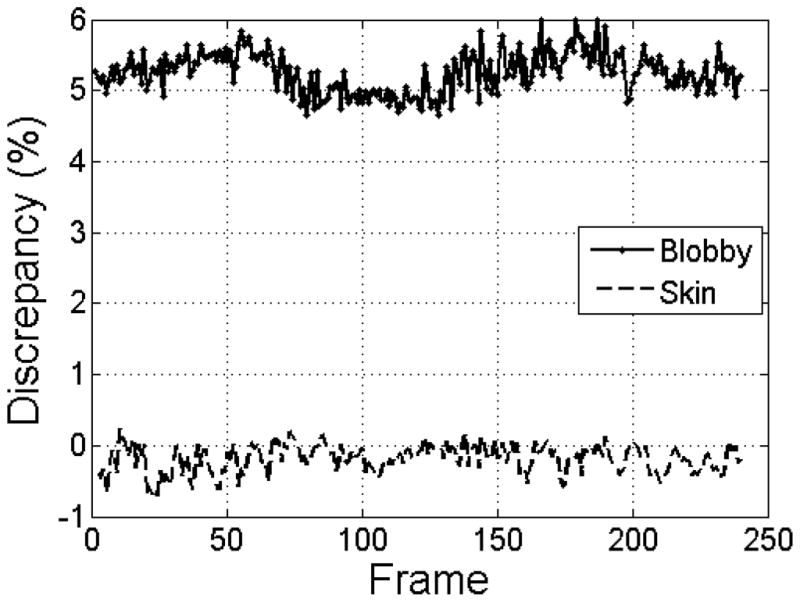
Comparison of surface area of skin and blobby surfaces versus Connolly MS for a dialanine trajectory: percentage difference is reported

4.2 Irregularity

Neither the skin nor the blobby surface presents self-intersections and consequent irregularities. However, it can be observed that there can still be very specific configurations where the normal vector to the skin is not defined. As shown in Figure 7, if compared to the Connolly surface, the singularity region is extremely limited, only one point, and it occurs only in a very specific conformation. For the blobby case non tangent continuity can also occur, due to a similarly pathological situation and to marching cubes artifacts.

Figure 7.

Pathological configurations for skin and blobby surface

4.3 Cavities and voids

In a third experiment, we analyze the presence of cavities and voids and assess the continuity of the surface area with respect to atomic positions. It is possible to observe, see for instance Figure 8 and the first panel of Figure 3, that both skin and blobby surfaces can generate internal spurious voids.

Figure 8.

Skin internal void (atoms patches were removed) and blobby internal void

It is possible to find a very interesting relationship between the presence of superficial voids, reflecting the non connectedness of the surface, and the continuity of the surface area with respect to atom center positions. In order to probe this hypothesis, we created an ad hoc geometric configuration, a sort of a “molecular basket”, where the non continuity of the Connolly surface area is evident; this model is the 3D counterpart of the 2D model described in [17]. The system is composed of 24 atoms organized on three parallel levels; each of them consists of 8 atoms of unitary radius whose radial distance is θ=π/4. The final result is a “basket” that can emulate the presence of an opening/closing cavity on the molecular surface. The x and z values for the first layer are computed as x=1.5cos(θ) and z=1.5sin(θ). The three layers are at a distance of 1.25Å. For the second and third layer one has x = βcos(θ) and z = βsin(θ) where β controls the opening of the cavity. For the Connolly surface the probe penetrates when β is around 2.4 while in the case of skin and blobby the basket opens when atoms are closer, for β around 1.45 and 1.35, respectively (in Figure 9 the opening process is shown while Figure 10 contains the surface area plots).

These experiments show that skin and blobby surface areas are continuous with respect to atom positions only if they include the areas of the internal voids and cavities. Since physical consistency requires filling these voids, the “corrected” versions would present a similar discontinuity to that found in the Connolly surface. Results on this simple model show, however, that the discontinuity of the Connolly surface is more pronounced. This aspect should be seriously considered and further analyzed when dealing with such surfaces. The correction step may become crucial when several voids are present: their ultimate effect, as observed by [9] for the blobby, is in fact to decrease the total energy due to an increase of the reaction field contribution. We further tested this phenomenon on a more realistic system, namely the crambin protein (PDB code 1CRN), using the OPLS2001 force field. We found that the total energy difference between the description based on the Connolly surface and the skin is around 6% due to a different shape and, more importantly, to the presence of artifactual voids arising from the skin definition. Unfortunately, it seems to be the case where correcting for physical inconsistency results in losing a desirable property such as surface area continuity with respect to atomic positions.

Summarizing this first analysis, we can conclude that the skin surface seems to be better suited for a good description of the SES than the blobby; reasonable suggestions for the parameter values are s =0.5 for the skin and the range B ∈ [−2.0, −3.0] for the blobby; the precise value for the latter depends on the desired level of smoothness.

4.4 Comparison with explicit solvent simulations

The aim of this section is to understand the behavior of skin and Connolly surfaces when they are used in the Finite Differences Poisson-Boltzmann based estimation of the electrostatic interaction energy in aqueous solvent as a function of the distance between prototypical charged moieties; similar experiments on the blobby surface were skipped, due to the results of the geometric observations made previously, which point to the intrinsic criticality of choosing a suitable B parameter and the consequent possible alteration of convex regions.

We focus on amino acid side chains already considered in [8] and in [9] and compare our results with the Potential of Mean Force calculated in these works. We therefore consider specific mutual orientations and different distances for the residue pairs indicated in Table 1, truncated at the C_β. For each configuration, we calculated the PBE electrostatic energy with the DelPhi solver and compared it to the PMF profile, neglecting the repulsive van der Waals contribution and focusing our attention on the distance at which maxima and minima are located; more detailed calculations should be done and a new PMF should be calculated in order to get more quantitative numbers concerning the energy values corresponding to these critical points. Table 1 summarizes the geometric mutual positioning of the residue pairs according to [8] and [9]. For any pair we computed the energy component derived from the electrostatic potential using two different force fields, namely OPLS2001 and CHARMM22. The s parameter of the skin surface was always set to 0.5 and the distance increment was set to 0.1Å, leading to 60/80 snapshots per pair.

Table 1.

Summary of the residue configurations: the first column contains the names of the residue pair and the corresponding figure, the second indicates the atoms used as reference when computing the distance r, the third column gives the approaching configuration while the last column reports the reference figure in [8] and [9]. Aminoacid superscripts indicate che charge state of the titratable residues.

Residues		Interface Atoms	Configuration	Reference
Arg+Glu−	Fig. 11	NH1 – Oε2	Coplanar double H-bond	Fig 3 in [8]
Lys+Glu−	Fig. 12	Nz – Cδ	Collinear	Fig 4a in [8]
Lys+Glu−	Fig. 12	Nz – Oε2	Side-to-Side	Fig 4b in [8]
His0Glu−	Fig. 13	Nδ1 – Oε2	Collinear H-bond	Fig 5b in [8]
His0His0	Fig. 14	Nε2 – Hδ1	Collinear	Fig 2 in [9]
Lys+Lys+	Fig. 15	Nz – Nz	Collinear	Fig 16 in [8]
Arg+Arg+	Fig. 16	Cz – Cz	Stacking	Fig 6a in [8]
Arg+Arg+	Fig. 16	NH1 – NH2	Collinear	Fig 6b in [8]

In figure 11 the Arginine-Glutamate pair is presented: the position of the first maximum of the explicit solvent is well tracked while the second minimum is not captured, regardless the used force field. Skin and Connolly surfaces produce a similar behavior, where the discrepancy in kcal/mol is never larger than 0.5. The spurious oscillations in the tail of the energy profile located in the right panel of Fig. 11 are due to the smallest atomic radius for Arginine in the CHARMM parameter set, which is about 0.22Å for some hydrogens and would require a computationally unviable grid spacing around 0.07Å.

Figure 11.

Energy profiles for Arg-Glu pair, OPLS2001 and CHARMM22 force fields.

In the first Lys⁺Glu⁻ pair (upper panels in Fig. 12) for CHARMM22 skin and Connolly surfaces are again very similar; instead using the OPLS2001 force field not only both skin and Connolly present a second minimum but in the case of the skin it is better positioned with respect to that obtained by the Connolly surface; in this respect it is interesting to observe that s = 0.5 leads to a skin surface whose area is usually smaller than that given by the Connolly MS with probe radius 1.4Å; this fact may in turn suggest that energy estimation in this case might benefit from a smaller probe radius. Incidentally, in [34] a probe radius of 0.8Å was used, leading to a good correspondence between RISM calculations [44] and Poisson-Boltzmann results for the cases K⁺Cl⁻, Na⁺Cl⁻ and Li⁺Cl⁻, where also the second minima were recovered. For the second orientation of the pair Lys⁺Glu⁻ (lower panels in Fig. 12) a second minimum is obtained but its positioning is not adequate with respect to explicit solvent results.

Figure 12.

Energy profile for the Lys-Glu pair in two different mutual orientations, OPLS2001 and CHARMM22 force fields

For the case His⁰Glu⁻ (figure 13) both surfaces and both force fields give qualitatively similar results, where the second minimum is not captured. For the case His⁰His⁰ results are in accordance with that obtained in [9] and do not detect the second minimum structure. However, in contrast to what observed by Swanson et al. in [9], high dielectric interstices do not occur in this experiment with the skin surface.

Figure 13.

Electrostatic potential for His-Glu pair, OPLS2001 and CHARMM22 force fields

The last tested cases consider repulsive pairs. All of them show agreement between skin and Connolly based results and additionally it is confirmed that they fail in capturing the two minima present in the PMF; this has already been observed, for instance, by Rashin et al. [34]. To verify that using a more accurate grid spacing does not affect the output, we tested a grid spacing of 0.17Å (DelPhi scale = 6.0); the results are shown in Figure 15. As already seen before, in the Arginine-Arginine pair (whose energy profiles are shown in Fig. 16) we found that the skin surface produces a little interstice in some configurations.

Figure 15.

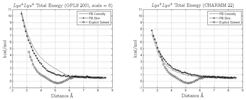
Energy profile for the Lys-Lys pair, OPLS2001 and CHARMM22 force fields

Figure 16.

Energy profile for Arg-Arg pair, OPLS2001 and CHARMM22 force fields

5 Conclusions

In this work, we analyzed some putative deficiencies of the Connolly-Richards [3, 4] molecular surface in the estimation of the electrostatic energy of biomolecular systems as mentioned in the literature as well as some possible alternative molecular surface definitions originating from the Computer Graphics scientific community. Our attention focused on the presence of regions where the normal is not defined, in a continuous dependence of the surface area on the atomic location and on the agreement with the upper level of theory in the simulation, represented by the explicit solvent models. During our analysis, we observed that adding a term in the Connolly model that mimics thermal motion can lead to a smoother surface with a well defined normal everywhere.

The considered alternative surfaces were the blobby surface [25], an example of implicit atom centered surfaces, and the skin surface [23]. In the first case we observed that, for any choice of the B parameter, it is far from trivial to match the expected shape of a solvent excluded surface for a given probe radius. In fact, due to its additive nature, modifying the parameter in order to fit reentrant regions can also alter solvent exposed convex patches resulting in unphysical shapes. In addition, the blobby surface can present some high dielectric interstices that can seriously affect the electrostatic energy estimation.

In the case of the skin surface, we found several attractive features, such as its analytical expression and the absence of self-intersections. Nevertheless, also the skin surface can lead to unwanted voids in the solute even in simple cases such as two interacting side chains. While it is true from its mathematical definition that the surface area of the skin is continuous with respect to atomic positions, we however observed that this property requires including the surface area of any internal cavity or void that might occur. Since assigning high dielectric to voids is unjustified from the physical viewpoint, this supposed value needs to be reconsidered. In terms of electrostatic energy estimation, we found that skin and Connolly provide comparable results with respect to explicit solvent based PMF. These results indicate that different MS definitions are unlikely to allow the reproduction of the behavior of structured solvent molecules occurring when the distance between the interacting moieties is larger than twice the probe radius. However, it is also plausible that tuning that definition can improve the description of the solvent behavior at closer distances. Choosing the correct molecular surface representation is a non trivial task and it depends on the problem at hand. Indeed for continuum implicit solvent models, molecular surfaces should be endowed with some useful geometric features such as those characterizing the blobby and the skin; nevertheless, a physically sound behavior ought to be maintained. The skin surface seems to better perform than the blobby in this respect although this latter is characterized by an intrinsically parallel nature and its computation can be ported proficiently on common GPUs [31], leading to a particularly fast implementation. On the numerical side, the skin surface involves the computation of the Voronoi diagram and of the mixed complex; both could be parallelized (in [29] the first step has already been implemented) but, despite these efforts, the skin computation will probably always be slower than the Connolly counterpart, as suggested in [29]. Additionally, if the skin surface is used analytically in the DelPhi solver, several demanding (although parallelizable) point-to-surface projections should be performed. Further analysis is currently in progress in order to transfer the advantages shown by these two definitions to a new model.

Figure 14.

Energy profile for the His-His pair, OPLS2001 and CHARMM22 force fields

Appendix

This appendix gives some details on skin surface definition and the projection technique employed.

In ℝ³ the mixed cell can be only of four types whereas in ℝ² only three types are allowed. For the ℝ³ case here we indicate by ν_l a Voronoi l-cell, by δ_k a Delaunay k-cell and by ${\mu }_{l,k}^s$ the mixed cell given by the sum of the previous two:

1. 1. ${\mu }_{3,0}^s=s·{\nu }_3\oplus (1-s)·{\delta }_0$

2. ${\mu }_{2,1}^s=s·{\nu }_2\oplus (1-s)·{\delta }_1$

3. ${\mu }_{1,2}^s=s·{\nu }_1\oplus (1-s)·{\delta }_2$

4. ${\mu }_{0,3}^s=s·{\nu }_0\oplus (1-s)·{\delta }_3$

These cells correspond informally to:

1. ${\mu }_{3,0}^s=s(\text{Voronoi}\text{Cell})\oplus (1-s)(\text{Delaunay}\text{Tetrahedron}\text{Vertex})$

2. ${\mu }_{2,1}^s=s(\text{Voronoi}\text{Facet})\oplus (1-s)(\text{Delaunay}\text{Tetrahedron}\text{Edge})$

3. ${\mu }_{1,2}^s=s(\text{Voronoi}\text{Edge})\oplus (1-s)(\text{Delaunay}\text{Tetrahedron}\text{Facet})$

4. ${\mu }_{0,3}^s=s(\text{Voronoi}\text{Vertex})\oplus (1-s)(\text{Delaunay}\text{Tetrahedron})$

Note that the Minkowsky sum is simple in all these cases: the first solid is a convex polyedron, the second is a prism with arbitrary base, the third is a prism with triangular base and the last is a tetrahedron.

Every mixed cell uniquely defines a patch over the surface; so there is a one-to-one correspondence between patches and mixed cells. The general surface equation corresponding to the cell ${\mu }_{l,k}^s$ is:

$$S_{{\mu }_{l,k}^s}(\mathbf{x})=\frac{1}{s-1}\sum _{i=1}^k{x}_i^2+\frac{1}{s}\sum _{i=k+1}^3{x}_i^2-\mathrm{\Delta }=0$$ (5.1)

The signed square distance Δ is defined as the power product between a vertex of the Delaunay tetraedrization (p(x,w)) (a weighted atom center) and the “focus” of the cell f associated to that cell:

$$\mathrm{\Delta }=w-{\left|\right|\mathbf{x}-\mathbf{f}\left|\right|}^2$$ (5.2)

The focus f of the cell is defined as:

1. For ${\mu }_{3,0}^s$ the focus is the Delaunay Tetrahedron Vertex

2. For ${\mu }_{2,1}^s$ the focus is the intersection between the Voronoi Facet and Delaunay Tetrahedron Edge

3. For ${\mu }_{1,2}^s$ the focus is the intersection between the Voronoi Edge and Delaunay Tetrahedron Facet

4. For ${\mu }_{0,3}^s$ the focus is the Voronoi vertex.

Depending on k (and thus l), each mixed cell is associated to the following surface equations up to proper roto-translations (these are detailed below):

1. $S_{{\mu }_{3,0}^s}(\mathbf{x}):x_1^2+x_2^2+x_3^3=s\mathrm{\Delta }$

2. $S_{{\mu }_{2,1}^s}(\mathbf{x}):\frac{1}{s-1}{x}_1^2+\frac{1}{s}{x}_2^2+\frac{1}{s}{x}_3^3=\mathrm{\Delta }$

3. $S_{{\mu }_{1,2}^s}(\mathbf{x}):\frac{1}{s-1}{x}_1^2+\frac{1}{s-1}{x}_2^2+\frac{1}{s}{x}_3^3=\mathrm{\Delta }$

4. $S_{{\mu }_{0,3}^s}(\mathbf{x}):x_1^2+x_2^2+x_3^3=(s-1)\mathrm{\Delta }$

For the constructions of the skin surface it is convenient to write down the quadric surface as a quadratic form such that:

$$S_{{\mu }_{l,k}^s}(\widehat{\mathbf{x}})={\widehat{\mathbf{x}}}^t\mathbf{Q}\widehat{\mathbf{x}}=0$$ (5.3)

Where x̂ =[x, 1]. In general given a rotation matrix R, a traslation matrix T and a surface matrix M such that the non roto-translate surface satisfies x̂^tMx̂ =0 one has:

$$\mathbf{Q}={({\mathbf{T}}^{-1})}^t·{({\mathbf{R}}^{-1})}^t·\mathbf{M}·{\mathbf{R}}^{-1}·{\mathbf{T}}^{-1}$$ (5.4)

Then one has:

$${\mathbf{Q}}_{{\mu }_{3,0}^s}=\left[\begin{array}{cccc}1& 0& 0& -f_1\\ 0& 1& 0& -f_2\\ 0& 0& 1& -f_3\\ -f_1& -f_2& -f_3& r_i^2+{\left|\right|f\left|\right|}^2\end{array}\right]{\mathbf{Q}}_{{\mu }_{0,3}^s}=\left[\begin{array}{cccc}1& 0& 0& -f_1\\ 0& 1& 0& -f_2\\ 0& 0& 1& -f_3\\ -f_1& -f_2& -f_3& (1-s)\mathrm{\Delta }+{\left|\right|f\left|\right|}^2\end{array}\right]$$ (5.5)

For hyperboloids instead proper roto-translations must be performed. The translation/rotation matrices are:

$$\mathbf{T}=\left[\begin{array}{cccc}1& 0& 0& f_1\\ 0& 1& 0& f_2\\ 0& 0& 1& f_3\\ 0& 0& 0& 1\end{array}\right]\mathbf{R}=\left[\begin{array}{cccc}{v}_1& u_1& w_1& 0\\ v_2& u_2& w_2& 0\\ v_3& u_3& w_3& 0\\ 0& 0& 0& 1\end{array}\right]$$ (5.6)

For the cell ${\mu }_{1,2}^s$ one sets w as the normalized vector that connects the two Voronoi vertexes of the Voronoi edge; v is a normalized vector that lies on the plane of the Delaunay facet; and u is the vector product of the previous two.

For the cell ${\mu }_{2,1}^s$ one sets v as the normalized vector that connects the two Delaunay vertexes of the Delaunay edge; w is a normalized vector that lies on the plane of the Voronoi facet; and u is the vector product of the previous two. These specifications allow to build the skin surface analytically.

In order to perform the projection to the quadric one can see that the problem can be formalized as a quadratic programming quadratically constrained minimization problem:

$$\{\begin{array}{c}{min}_{\widehat{\mathbf{x}}}{\left|\right|\widehat{\mathbf{y}}-\widehat{\mathbf{x}}\left|\right|}^2\\ {\widehat{\mathbf{x}}}^t\mathbf{A}\widehat{\mathbf{x}}+2{\mathbf{a}}^t\widehat{\mathbf{x}}+a_0=0\end{array}$$ (5.7)

If we assume that the reference system is given by the quadric then a vanishes and A is diagonal with elements A₁, A₂, A₃. Thus we are assuming that the point y is roto-translated as per ŷ =(TR)⁻¹y. One can proceed [45] by using a Lagrangian whose Lagrange multiplier is α thus getting as a first optimality condition:

$$\widehat{\mathbf{x}}={(\mathbf{I}+\alpha \mathbf{A})}^{-1}\mathbf{y}$$ (5.8)

Substituting this last equation in the quadric equation provides the searched polynomial. It can be shown after some algebraic manipulations that the polynomial to be solved in α is given by the following coefficients in decreasing degree order:

$$\{\begin{array}{c}{c}_6=a_0{A}_1^2{A}_2^2{A}_3^2\\ c_5=2a_0{A}_1{A}_2{A}_3(A_2{A}_3+A_1{A}_3+A_1{A}_2)\\ c_4={\widehat{y}}_1^2{A}_1{A}_2^2{A}_3^2+a_0{A}_2^2{A}_3^2+{\widehat{y}}_2^2{A}_1^2{A}_2{A}_3^2+4a_0{A}_1{A}_2{A}_3^2+a_0{A}_1^2{A}_3^2+\\ {\widehat{y}}_3^2{A}_1^2{A}_2^2{A}_3+4a_0{A}_1{A}_2^2{A}_3+4a_0{A}_1^2{A}_2{A}_3+a_0{A}_1^2{A}_2^2\\ c_3=2({\widehat{y}}_2^2{A}_1{A}_2{A}_3^2+{\widehat{y}}_1^2{A}_1{A}_2{A}_3^2+a_0{A}_2{A}_3^2+a_0{A}_1{A}_3^2+{\widehat{y}}_3^2{A}_1{A}_2^2{A}_3+\\ {\widehat{y}}_1^2{A}_1{A}_2^2{A}_3+a_0{A}_2^2{A}_3+{\widehat{y}}_3^2{A}_1^2{A}_2{A}_3+{\widehat{y}}_2^2{A}_1^2{A}_2{A}_3+4a_0{A}_1{A}_2{A}_3+\\ a_0{A}_1^2{A}_3+a_0{A}_1{A}_2^2+a_0{A}_1^2{A}_2)\\ c_2={\widehat{y}}_2^2{A}_2{A}_3^2+{\widehat{y}}_1^2{A}_1{A}_3^2+a_0{A}_3^2+{\widehat{y}}_3^2{A}_2^2{A}_3+4{\widehat{y}}_3^2{A}_1{A}_2{A}_3+\\ 4{\widehat{y}}_2^2{A}_1{A}_2{A}_3+4{\widehat{y}}_1^2{A}_1{A}_2{A}_3+4a_0{A}_2{A}_3+{\widehat{y}}_3^2{A}_1^2{A}_3+4a_0{A}_1{A}_3+\\ {\widehat{y}}_1^2{A}_1{A}_2^2+a_0{A}_2^2+{\widehat{y}}_2^2{A}_1^2{A}_2+4a_0{A}_1{A}_2+a_0{A}_1^2\\ c_1=2({\widehat{y}}_3^2{A}_2{A}_3+{\widehat{y}}_2^2{A}_2{A}_3+{\widehat{y}}_3^2{A}_1{A}_3+\\ {\widehat{y}}_1^2{A}_1{A}_3+a_0{A}_3+{\widehat{y}}_2^2{A}_1{A}_2+{\widehat{y}}_1^2{A}_1{A}_2+a_0{A}_2+a_0{A}_1\\ c_0={\widehat{y}}_3^2{A}_3+{\widehat{y}}_2^2{A}_2+{\widehat{y}}_1^2{A}_1+a_0\end{array}$$ (5.9)

After finding the sixth roots of the previous polynomial one recovers the sixth candidate points by (3.6) and keeps the point with minimum distance with respect to ŷ. Finally, the projected point is x = TRx̂.

References

- 1.Fogolari F, Brigo A, Molinari H. The poissonboltzmann equation for biomolecular electrostatics: a tool for structural biology. J Mol Recognit. 2002;15:377392. doi: 10.1002/jmr.577. [DOI] [PubMed] [Google Scholar]
- 2.Onufriev A, Bashford D, Case DA. Effective born radii in the generalized born approximation: The importance of being perfect. J Comp Chem. 2002;23(14):12971304. doi: 10.1002/jcc.10126. [DOI] [PubMed] [Google Scholar]
- 3.Lee B, Richards FM. The interpretation of protein structures: estimation of static accessibility. J Mol Biol. 1971;55:379400. doi: 10.1016/0022-2836(71)90324-x. [DOI] [PubMed] [Google Scholar]
- 4.Connolly ML. Analytical molecular surface calculation. J Appl Cryst. 1983;16:548–558. [Google Scholar]
- 5.Sanner MF, Olson AJ, Spehner JC. Reduced surface: An efficient way to compute molecular surfaces. Biopolymers. 1996;38:305320. doi: 10.1002/(SICI)1097-0282(199603)38:3%3C305::AID-BIP4%3E3.0.CO;2-Y. [DOI] [PubMed] [Google Scholar]
- 6.Rocchia W, Sridharan S, Nicholls A, Alexov E, Chiabrera A, Honig B. Rapid grid-based construction of the molecular surface for both molecules and geometric objects: Applications to the finite difference poisson-boltzmann method. J Comp Chem. 2002;23:128–137. doi: 10.1002/jcc.1161. [DOI] [PubMed] [Google Scholar]
- 7.Totrov M, Abagyan R. The contour-buildup algorithm to calculate the analytical molecular surface. Journal of Structural Biology. 1996;116:138143. doi: 10.1006/jsbi.1996.0022. [DOI] [PubMed] [Google Scholar]
- 8.Masunov A, Lazaridis T. Potentials of mean force between ionizable amino acid side chains in water. Journal of the American Chemical Society. 2003;125:1722–1730. doi: 10.1021/ja025521w. [DOI] [PubMed] [Google Scholar]
- 9.Swanson JMJ, Mongan J, McCammon A. Limitations of atom-centered dielectric functions in implicit solvent models. The Journal of Physical Chemistry B. 2005;109:14769–14772. doi: 10.1021/jp052883s. [DOI] [PubMed] [Google Scholar]
- 10.Rocchia W, Alexov E, Honig B. Extending the applicability of the nonlinear poisson-boltzmann equation: Multiple dielectric constants and multivalent ions. J Phys Chem B. 2001;105(28):6507–6514. [Google Scholar]
- 11.Xu D, Zhang Y. Generating triangulated macromolecular surfaces by euclidean distance transform. PLoS One. 2009;4 doi: 10.1371/journal.pone.0008140. [DOI] [PMC free article] [PubMed] [Google Scholar]
- 12.Can T, Chen C, Wang YF. Efficient molecular surface generation using level-set methods. Journal of Molecular Graphics and Modelling. 2006;25:442454. doi: 10.1016/j.jmgm.2006.02.012. [DOI] [PubMed] [Google Scholar]
- 13.Bardhan JP, Altman MD, Willis DJ, Lippow SM, Tidor B, White JK. Numerical integration techniques for curved-element discretizations of molecule-solvent interfaces. The Journal Of Chemical Physics. 2007;127 doi: 10.1063/1.2743423. [DOI] [PMC free article] [PubMed] [Google Scholar]
- 14.Bajaj C, Lee H, Merkert R, Pascucci V. Nurbs based b-rep models from macromolecules and their properties. Fourth Symposium on Solid Modeling and Applications. 1997:217–228. [Google Scholar]
- 15.Liang J, Edelsbrunner H, Fu P, Sudhakar PV, Subramaniam S. Analytical shape computation of macromolecules: Molecular area and volume through alpha shape. Proteins. 1998;33:117. [PubMed] [Google Scholar]
- 16.Ryua JR, Kimb DS. Molecular surfaces on proteins via beta shapes. Computer-Aided Design. 2007;39:10421057. [Google Scholar]
- 17.Lu Q, Luo R. A poissonboltzmann dynamics method with nonperiodic boundary condition. Journal of Chemical Physics. 2003;119:11035–11047. [Google Scholar]
- 18.Vorobjev YN, Hermans J. Sims: Computation of a smooth invariant molecular surface. Biophysical Journal. 1997;73:722–732. doi: 10.1016/S0006-3495(97)78105-0. [DOI] [PMC free article] [PubMed] [Google Scholar]
- 19.Bates PW, Wei GW, Zhao S. Minimal molecular surfaces and their applications. Journal of Computational Chemistry. 2008;29(3):380391. doi: 10.1002/jcc.20796. [DOI] [PubMed] [Google Scholar]
- 20.Lorensen WE, Cline HE. Marching cubes: A high resolution 3d surface construction algorithm. Computer Graphics. 1987;21(4) [Google Scholar]
- 21.Grant JA, Pickup BT, Nicholls A. A smooth permittivity function for poissonboltzmann solvation methods. Journal of Computational Chemistry. 2001;22(6):608640. [Google Scholar]
- 22.Im W, Beglov D, Roux B. Continuum solvation model: computation of electrostatic forces from numerical solutions to the poisson-boltzmann equation. Comput Phys Commun. 1998;111(59):59–75. [Google Scholar]
- 23.Edelsbrunner H. Deformable smooth surface design. Discrete and Computational Geometry. 1999;21(1):87–115. [Google Scholar]
- 24.Blinn JF. A generalization of algebraic surface drawing. ACM Transactions on Graphics. 1982;1(3):235–256. [Google Scholar]
- 25.Zhang Y, Xu G, Bajaj C. Quality meshing of implicit solvation models of biomolecular structures. Computer Aided Geometric Design. 2006;23:510530. doi: 10.1016/j.cagd.2006.01.008. [DOI] [PMC free article] [PubMed] [Google Scholar]
- 26.Cheng HL, Shi X. Quality mesh generation for molecular skin surfaces using restricted union of balls. IEEE Visualization. 2005 [Google Scholar]
- 27.Kruithof NGH, Vegter G. Meshing skin surfaces with certified topology. Computational Geometry: Theory and Applications. 2007;36(3) [Google Scholar]
- 28.Chavent M, Levy B, Maigret B. Metamol: High quality visualization of molecular skin surface. Journal of Molecular Graphics and Modelling. 2008;27(2):209–216. doi: 10.1016/j.jmgm.2008.04.007. [DOI] [PubMed] [Google Scholar]
- 29.Lindow N, Baum D, Prohaska S, Hege HC. Accelerated visualization of dynamic molecular surfaces. Eurographics/IEEE-VGTC Symposium on Visualization. 2010;29:943–951. [Google Scholar]
- 30.Holst M, Saied F. Multigrid solution of the poisson-boltzmann equation. J Comput Chem. 1993;14:105–113. [Google Scholar]
- 31.Agostino D, Decherchi S, Galizia A, Colmenares J, Quarati A, Rocchia W, Clematis A. Cuda accelerated blobby molecular surface generation. In accepted at PPAM. 2011 [Google Scholar]
- 32.Bashford D. An object-oriented programming suite for electrostatic effects in biological molecules, an experience report on the mead project. In Scientific Computing in Object-Oriented Parallel Environments, Lecture Notes in Computer Science. 1997;1343:233–240. [Google Scholar]
- 33.Bajaj CL, Pascucci V, Shamir A, Holt RJ, Netravali AN. Dynamic maintenance and visualization of molecular surfaces. Discrete Applied Mathematics. 2003;127(1) [Google Scholar]
- 34.Rashin AA, Iofin M, Honig B. Internal cavities and buried waters in globular proteins. Biochemistry. 1986;25(12):36193625. doi: 10.1021/bi00360a021. [DOI] [PubMed] [Google Scholar]
- 35.Cheng HL, Dey TK, Edelsbrunner H, Sullivan J. Dynamic skin triangulation. Discrete Comput Geom. 2001;25:525–568. [Google Scholar]
- 36.Rycroft CH. Voro++: A three-dimensional voronoi cell library in c++ Chaos. 2009;19(4) doi: 10.1063/1.3215722. [DOI] [PubMed] [Google Scholar]
- 37.Eberly D. Distance from point to a general quadratic curve or a general quadric surface. Geometric Tools. http://www.geometrictools.com/
- 38.Kazhdan M, Bolitho M, Hoppe H. Poisson surface reconstruction. Eurographics Symposium on Geometry Processing. 2006 [Google Scholar]
- 39.Desbrun M, Meyer M, Schröder P, Barr AH. Discrete differential-geometry operators for triangulated 2-manifolds. VisMath. 2002;2:35–57. [Google Scholar]
- 40.An adaptive MLS surface for reconstruction with guarantees. 2005. [Google Scholar]
- 41.ReMESH: An Interactive Environment To Edit And Repair Triangle Meshes. 2006. [Google Scholar]
- 42.Cignoni P, Rocchini C, Scopigno R. Metro: measuring error on simplified surfaces. Computer Graphics Forum. 1998;17(2):167–174. [Google Scholar]
- 43.Pietrucci F, Broglia RA, Bonomi M, Branduardi D, Bussi G, Camilloni C, Provasi D, Raiteri P, Donadio D, Marinelli F, Parrinello M. Plumed: a portable plugin for free energy calculations with molecular dynamics. Comp Phys Comm. 2009;180(1961) [Google Scholar]
- 44.Pettitt BM, Rossky PJ. Alkali halides in water: Ion-solvent correlations and ion-ion potentials of mean force at infinite dilution. J Chem Phys. 1986;84(5836) [Google Scholar]
- 45.Lennerz C, Schomer E. Efficient distance computation for quadratic curves and surfaces. Geometric Modeling and Processing: Theory and Applications. 2002 [Google Scholar]