Abstract
A method for determining the pupil phase distribution of an optical system is demonstrated. Coefficients in a wavefront expansion were estimated using likelihood methods, where the data consisted of multiple irradiance patterns near focus. Proof-of-principle results were obtained in both simulation and experiment. Large-aberration wavefronts were handled in the numerical study. Experimentally, we discuss the handling of nuisance parameters. Fisher information matrices, Cramér-Rao bounds, and likelihood surfaces are examined. ML estimates were obtained by simulated annealing to deal with numerous local extrema in the likelihood function. Rapid processing techniques were employed to reduce the computational time.
OCIS codes: (100.5070) Phase retrieval, (120.5050) Phase measurement, (120.3940) Metrology
1. Introduction
Phase retrieval (PR) is a useful method for recovering the phase distribution in the pupil of an optical system from the irradiance distribution in the focal plane. However, the usual PR problem is ill posed, since both distributions are unrestricted 2D functions [1] and a single irradiance measurement does not ensure that the recovered phase is unique [2,3]. A straightforward solution to avoid the ambiguities is to make multiple irradiance measurements near the focal plane, where the minimum number of planes is two.
Another approach to avoiding the phase ambiguities is to estimate the parameters describing the phase function, instead of the function itself [4–6]. Parameterization of the phase is achieved with a set of expansion functions. Obvious choices for circular pupils are Zernike polynomials, although there are many other options.
In our method, the data consist of irradiance measurements in multiple planes near the focus of an aberrated optical element (Fig. 1 ). From the multifocal data, we estimate the coefficients of phase polynomials in a wavefront expansion, as proposed by Brady and Fienup [4–6], but with various extensions. We use maximum-likelihood estimation (MLE) for the estimation procedure, which enables us to optimize the data-acquisition system by analyzing the Fisher information matrix and associated Cramér-Rao lower bound, as well as likelihood surfaces. Additionally, we have developed our method to handle very large wavefront aberrations. To deal with the high computational demand of the estimation step, we employ rapid-processing techniques using dedicated computer hardware.
Fig. 1.
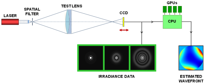
Data-acquisition system for collecting multiple irradiance patterns near the focus of an optical element.
2. Propagation algorithm
The form of the diffraction integral, without the Fresnel approximation, used in this paper is
| (1) |
where r0 and r are two-dimensional vectors in the pupil and image planes, respectively [7,8]. It is a version of the Huygens wavelet formulation when the obliquity factor in the integral is neglected and distance is replaced by z in the denominator. Thus, the field at each observation point in the image plane is the sum of an infinite number of secondary waves emanating from the aperture. Since the integrand of the double integral in Eq. (1) can vary rapidly over the integration domain, especially when the aberrations are large, a significant amount of sampling in the aperture is required to accurately predict the irradiance distribution in the image plane. Consequently, numerical evaluations of the Huygens diffraction integral are prohibitively time-consuming and an approximation to this integral is necessary to reduce the computing problem.
Note that both the Huygens wavelet formation and the Fresnel approximation assume scalar diffraction theory, which we assume to be adequate for our method of wavefront measurement with multifocal data, even when large aberrations are present.
Suppose a converging wave has wavefront error in the exit pupil of an optical system. Then the field in the exit pupil is given by
| (2) |
where and f is defined as the radius of curvature of the unaberrated wave in the exit pupil (i.e., the distance between the exit pupil and paraxial focus). Inserting Eq. (2) into Eq. (1) leads to
| (3) |
or equivalently,
| (4) |
where the last exponential term is part of the integrand. A binomial expansion for and leads to
| (5) |
where HOT denotes the higher-order terms in :
| (6) |
Combining Eq. (4) and Eq. (5) results in
| (7) |
where the function A(r) is given by
| (8) |
If the higher-order terms in Eq. (7) can be ignored, that equation can be represented by a 2D Fourier transform, known as the Fresnel approximation:
| (9) |
where the spatial frequency is . The corresponding irradiance under this approximation is given by
| (10) |
The approximation in Eq. (9) breaks down as the numerical aperture of the optical system increases. Under circumstances when the higher-order terms are not negligible, we might consider including, say, the fourth-order terms in Eq. (6). A limitation is that r and r0 are inseparable in these terms, so including them in the integral means that we cannot take advantage of the FFT. Since a brute-force computation of the diffraction integral is too computationally expensive and impractical, the best we can do is minimize the terms in Eq. (6) by considering planes sufficiently close to nominal focus, so that z ≈f and r is small.
3. Parameterized wavefront description
The unknown function of interest in these equations is the wavefront error , which we represent in a parameterized form in the exit pupil of the optical system. Our approach is based on the fundamental assumption that the continuous wavefront can be approximated to sufficient accuracy by a finite set of expansion functions. We choose to represent this function by expanding it in some number of Zernike polynomials,
| (11) |
where is the nth polynomial with coefficient .
The parameters to be estimated are the Zernike coefficients {αn, n = 1,…, N), but an important determination is the number of coefficients necessary for an accurate representation of the wavefront. Even if a small number of terms is used in the expansion, this does not imply that the wavefront aberration is small; representing large wavefront errors simply requires large coefficients. In our approach, we assume that the wavefront is smoothly varying, so that sufficient accuracy can be achieved with a relatively small value of N.
4. Maximum-likelihood estimation
Algorithms that implement the ML approach to estimating a vector set of parameters θ perform a search through the space defined by all possible values to find a point that maximizes the likelihood, or probability, of generating the observed data vector g:
| (12) |
Here, represents the ML estimates and is the probability of the data vector g, conditioned on the set of parameters θ. Essentially all search algorithms locate an extremum via iterative methods that execute in a variable number of steps depending on the starting location, the volume of the search space, the complexity of the probability surface, and values selected for convergence factors. Since we are dealing with a complicated likelihood surface in a high-dimensional space with many local minima, we implement a global search algorithm called simulated annealing (SA) that can be tailored to the probability surface [9]. The major criticism of simulated annealing is its lengthy computational time, but it is very effective in finding a good approximation to the global optimum of a complicated cost function.
In estimation theory, bias and variance are used to specify estimator performance, where bias is defined as the deviation of the average parameter estimate from the true value, and variance is the mean-square fluctuation of the estimate about its mean. In essence, bias is related to accuracy and variance to precision. Inherent bias in the estimator and systematic errors due to miscalibration or inaccurate modeling of the system both factor into the overall bias. Variance provides a measure of random errors that fluctuate from one measurement to another for a given wavefront.
Immediate advantages of ML estimation are that it is efficient (i.e., unbiased and yields the best possible variance), if an efficient estimator exists, and that it is asymptotically efficient as more or better data are acquired. Furthermore, its performance can be analyzed with the Fisher information matrix (FIM), which can be used to design and optimize the system that acquires the data to be used as input to the estimation routine. One major challenge in ML estimation is that an accurate probability model must be used that includes all sources of randomness (e.g., photon noise and electronic noise).
A significant limitation to be overcome is that the ML estimation step is very time-consuming, so making it practical requires rapid processing techniques and dedicated computer hardware. Improvement of computational time can be achieved by parallelizing the propagation algorithm describing the forward model of the system. Parallel algorithms can be implemented on a variety of hardware platforms, including the graphics processing unit (GPU) in video cards, capable of massively parallel high-performance computing in scientific and engineering fields. Modern GPU programming is accomplished using an extension to the C programming language, CUDA (“Compute Unified Device Architecture”), which provides software development tools and allows functions in C to be implemented on a GPU’s multiple stream processors.
Since the logarithm increases monotonically with its argument, Eq. (12) can be rewritten as
| (13) |
For a purely Gaussian noise model with independent and identically distributed (i.i.d.) detector elements, it can be shown that ML estimation according to Eq. (13) reduces to nonlinear least-squares fitting between the data and the output of the optical design program:
| (14) |
Since the data-acquisition system described in this work was not photon-starved, we assumed that it was dominated by electronic noise, which is adequately described by Gaussian statistics.
5. Fisher information and Cramér-Rao bounds
The performance of the ML estimator can be analyzed with the Fisher information matrix, denoted F, since it describes the ability to estimate a vector set of parameters and is related to the sensitivity of the data to changes in those parameters. For a vector parameter of P real components, the FIM is a P × P symmetric matrix with components Fjk given by
| (15) |
where the angle brackets denote the average [7]. Mathematically, F is the covariance matrix of the gradient of the logarithm of the likelihood, so that the off-diagonal entries indicate undesirable coupling between different pairs of parameters; stronger coupling leads to greater noise in the estimates. The derivative of the log-likelihood with respect to θ is the score.
For Gaussian i.i.d. data, the FIM components reduce to
| (16) |
which depend on the average data vector evaluated at the set of parameters and are inversely proportional to the variance in the detector elements [7,10].
Inversion of the FIM provides the Cramér-Rao lower bound (CRB) on the variance (i.e. the theoretical minimum possible variance) of the parameter estimates. It is well-documented in the literature that the variance of any unbiased estimate obeys the Cramér-Rao inequality [11,12], written as
| (17) |
where is the pth parameter and is the covariance matrix of the estimates. For an efficient estimator, the inverse of the FIM is the covariance matrix of the parameter estimates; thus, its off-diagonal elements represent coupling between these estimates.
In general, the FIM can be computed for any system configuration and therefore be used to design and optimize the system that acquires the data to be used as input to the estimation procedure. Additionally, data from multiple image planes may serve to reduce parametric coupling, which could improve parameter estimability.
6. Numerical results
6.1 Test lens description
For the numerical proof-of-principle system, we chose a large nine-surface unit lens for use in a larger assembly. We operated the rotationally-symmetric lens at finite conjugates by placing an on-axis point source at 113.0 mm from the entrance pupil. According to ZEMAX, the exit pupil diameter and working f-number were Dxp = 88.41 mm and f/#w = 1.796, respectively, at the wavelength λ = 0.6328 μm. The peak-to-valley wavefront error was 149.1λ.
We chose to expand the wavefront in terms of the Fringe Zernike polynomials, which are identical to the standard polynomials, except for the indexing format and the order in which they are listed. The Fringe Zernike coefficients describing in the exit pupil were calculated in ZEMAX for N = 37, the maximum number of terms (Table 1 ). Since the system has rotational symmetry, the coefficients for all non-rotationally symmetric Zernike terms are zero; thus non-zero coefficients correspond to piston, defocus, and various orders of spherical aberration. Table 2 provides the polynomial expressions for {Zn, n = 1,…,9, 16, 25, 36, 37}, corresponding to the rotationally symmetric terms and several low-order terms.
Table 1. Fringe Zernike coefficients {αn, n = 1,…, 37}, peak-to-valley, RMS, and variance, provided by ZEMAX for the highly aberrated test lens. Unlisted coefficients are zero.
| Index | Aberration Type [λ] | Design Value [λ] |
|---|---|---|
| 1
|
Piston
|
50.73020573
|
| 4
|
Defocus
|
75.17884184
|
| 9
|
Spherical Aberration, Primary
|
23.81690475
|
| 16
|
Spherical Aberration, Secondary
|
−0.60555615
|
| 25
|
Spherical Aberration, Tertiary
|
0.04113341
|
| 36
|
Spherical Aberration, Quaternary
|
−0.00287742
|
| 37
|
Spherical Aberration,
12th-order Term
|
−0.01310320
|
| Peak-to-valley [λ]
|
N/A
|
149.14956942
|
| RMS [λ]
|
N/A
|
44.18240916
|
| Variance [λ2] | N/A | 1952.08527937 |
Table 2. Fringe Zernike Polynomials {Zn, n = 1,…, 9, 16, 25, 36, 37}.
| n | Fringe Zernike Polynomial | Aberration Type |
|---|---|---|
| 1
|
1
|
Piston
|
| 2
|
ρcosθ
|
Distortion - Tilt (x-axis)
|
| 3
|
ρsinθ
|
Distortion - Tilt (y-axis)
|
| 4
|
2ρ
2 − 1
|
Defocus - Field Curvature
|
| 5
|
ρ
2cos2θ
|
Astigmatism, Primary (0° or 90°)
|
| 6
|
ρ
2sin2θ
|
Astigmatism, Primary ( ± 45°)
|
| 7
|
(3ρ
3 − 2ρ)cos2θ
|
Coma, Primary (x-axis)
|
| 8
|
(3ρ
3 − 2ρ)sin2θ
|
Coma, Primary (y-axis)
|
| 9
|
6ρ
4 − 6ρ
2 + 1
|
Spherical Aberration, Primary
|
| 16
|
20ρ
6 − 30ρ
4 + 12ρ
2 − 1
|
Spherical Aberration, Secondary
|
| 25
|
70ρ
8 − 140ρ
6 + 90ρ
4 − 20ρ
2 + 1
|
Spherical Aberration, Tertiary
|
| 36
|
252ρ
10 − 630ρ
8 + 560ρ
6 − 210ρ
4 + 30ρ
2 − 1
|
Spherical Aberration, Quaternary
|
| 37 | 924ρ 12 − 2772ρ 10 + 3150ρ 8 − 1680ρ 6 + 420ρ 4 − 42ρ 2 + 1 | Spherical Aberration, 12th order |
6.2 Irradiance data
A critical design option is the number and location of planes at which to measure the irradiance. It is well known that two-plane measurements are sufficient to determine the pupil phase, so to minimize computation time, we selected two output planes just before paraxial focus, z = z1 = zf – 0.25 mm and z = z2 = zf – 0.43 mm, where the paraxial focal plane is located at z = zf = 157.8 mm and the exit pupil lies in the z = 0 plane. So that each irradiance distribution provided unique information, special care was taken to select planes sufficiently far from each other, yet close enough to the nominal focus for the approximation in Eq. (9) to hold.
For both planes, we determined that the minimum level of pupil sampling to accurately represent the irradiance data was 1024 × 1024. Essentially, output planes farther from focus and larger aberrations in the test lens require greater sampling. We added zero-padding for a final FFT grid size of 2048 × 2048, which was used to compute the irradiance data in Fig. 2 . The detector element spacing was roughly 0.56 μm based on these grid sizes.
Fig. 2.
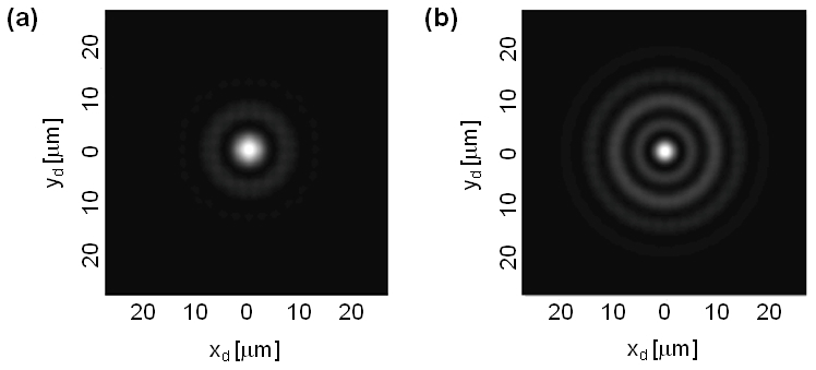
Detector data for the highly aberrated test lens using a pupil sampling of P = 1024 at image plane: (a) z = z1 and (b) z = z2.
6.3 Fisher information and Cramér-Rao bounds
We computed the FIM using Eq. (16) for the parameters we wanted to estimate, the Fringe Zernike coefficients {αn, n = 2,…, 9, 16}, shown in Fig. 3(a) on a logarithmic scale. Although the off-axis coefficients included here are zero in this idealized case, in a real system, they may become non-zero if there are any system misalignments. Since α1 corresponds to piston and does not influence the irradiance data, we had no interest in estimating it and disregarded it in the FIM. The variance σ2 in the detector elements was based on a peak SNR of 104. We evaluated the FIM components at θ, based on the values in Table 1. Note that the FIM is a 9 × 9 symmetric matrix and is order-specific, with the parameter indices on the x and y axes. The jkth entry has units of
Fig. 3.
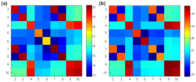
(a) FIM and (b) its inverse, for Fringe Zernike coefficients {αn, n = 2,…, 9, 16} in the exit pupil of the highly aberrated test lens. Shown on a logarithmic scale.
| (18) |
In a real physical system, the coefficients related to tilt and off-axis aberrations (i.e., coma and astigmatism) would be useful in determining misalignments in the optical system, while the remaining coefficients represent defocus and spherical aberration, relating to optical power and the curvatures and asphericities of the refractive surfaces.
High diagonal values in the FIM indicated that there was substantial information in the data for each parameter. However, the pronounced off-diagonal structure revealed strong parametric coupling between the pairs (2,7), (3,8), (4,9), (4,16), and (9,16), which would only confound the estimation problem. Note that the degree of coupling between two parameters is proportional to the magnitude of the respective FIM component.
We computed the inverse of the FIM, shown in Fig. 3(b), and read off its diagonal components to determine the CRB for the parameters, whose square-root is provided in Table 3 . The diminutive values in (CRB)1/2, on the order of 10−10 to 10−9, permit the estimation of the wavefront parameters to very high precision, provided that the forward model is exact.
Table 3. Square-root of the CRB for Fringe Zernike coefficients {αn, n = 2,…, 9, 16} in the exit pupil of the highly aberrated test lens at λ = 0.6328 μm. Units are in waves λ.
| Index | (CRB)1/2 [λ] | Index | (CRB)1/2 [λ] |
|---|---|---|---|
| 2
|
6.6 × 10⁻¹⁰
|
7
|
3.6 × 10⁻¹⁰
|
| 3
|
6.6 × 10⁻¹⁰
|
8
|
3.6 × 10⁻¹⁰
|
| 4
|
1.2 × 10⁻¹⁰
|
9
|
2.2 × 10⁻⁹
|
| 5
|
6.8 × 10⁻¹⁰
|
16
|
1.5 × 10⁻¹⁰
|
| 6 | 1.5 × 10⁻⁹ |
6.4 Likelihood surfaces
When solving optimization problems, it helps to have a strong sense of the objective function to be optimized. This is particularly useful when fitting nonlinear, multivariate functions that may be plagued with numerous local extrema.
In the context of ML estimation, a plot of pr(g|θ ) versus θ for a particular g is called the likelihood surface for that data vector. Although we are minimizing the sum-of-squares (i.e., negative likelihood), we will refer to this objective function as the likelihood surface.
For a vector set of N parameters, the likelihood surface exists in an N-dimensional hyperspace. However, we are restricted to plotting the likelihood surface while varying up to two parameters at a time. We selected a handful of pairs of parameters for the following plots (Fig. 4 ) and applied the ranges given in Table 4 . In each plot, the fixed parameters were set to the true values underlying the data.
Fig. 4.
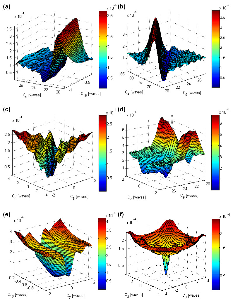
Likelihood surface plotted along two axes at a time for pairs of parameters: (a) α9 and α16, (b) α4 and α9, (c) α3 and α8, (d) α7 and α9, (e) α7 and α16, and (f) α2 and α3.
Table 4. Range in likelihood surface plots for Fringe Zernike coefficients {αn, n = 2,…, 9, 16} in the exit pupil of the highly aberrated test lens. Units are in waves.λ.
| Index | True value [λ] | Range |
|---|---|---|
| 2
|
0
|
± 4λ
|
| 3
|
0
|
± 4λ
|
| 4
|
75.17884184
|
± 10λ
|
| 5
|
0
|
± 4λ
|
| 7
|
0
|
± 2λ
|
| 8
|
0
|
± 2λ
|
| 9
|
23.81690475
|
± 4λ
|
| 16 | −0.60555615 | ± λ/2 |
6.5 Maximum-likelihood estimates
After generating the data (Fig. 2), we disregarded our knowledge of Zernike coefficients {αn, n = 2,…, 9, 16}, then estimated them using ML estimation according to our Gaussian noise model. Upper and lower limits in the search space were based on the specified ranges in Table 4. We generated a random starting point, as provided in Table 5 .
Table 5. ML estimates of wavefront parameters for the highly aberrated test lens at λ = 0.6328 μm, including their standard deviations and the starting point in the search. Units are in waves λ.
| Index | True Value [λ] | Start Point [λ] | Estimate [λ] |
|---|---|---|---|
| 2
|
0
|
2.33765863
|
0.11 ± 0.34
|
| 3
|
0
|
3.67593941
|
−0.09 ± 0.30
|
| 4
|
75.17884184
|
81.29481398
|
75.5 ± 1.0
|
| 5
|
0
|
−3.71430657
|
−0.09 ± 0.28
|
| 6
|
0
|
2.79303444
|
0.17 ± 0.23
|
| 7
|
0
|
1.73597299
|
0.08 ± 0.33
|
| 8
|
0
|
−1.81531443
|
−0.10 ± 0.36
|
| 9
|
23.81690475
|
20.60294575
|
23.58 ± 0.59
|
| 16 | −0.60555615 | −0.29345783 | −0.604 ± 0.047 |
We ran 12 optimization trials, with each trial representing a distinct noise realization for the same wavefront parameters, and implemented the same estimation procedure on each. Figure 5 illustrates the optimal cost function versus iteration number for the trials, starting at the end of the first temperature phase. The average final cost and number of temperature phases were 147.7 and 87.3, respectively. This number of phases is equivalent to a final temperature of 116.1.
Fig. 5.
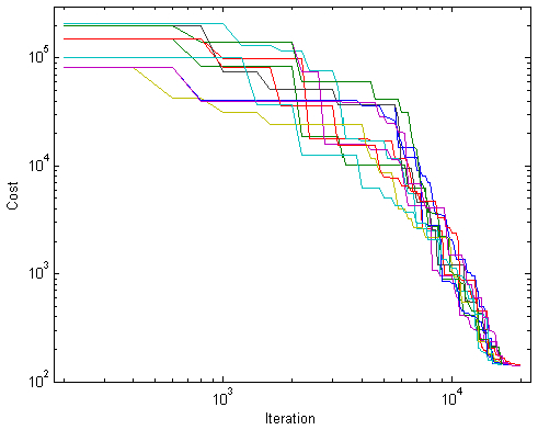
12 simulated annealing trials for the estimation of wavefront parameters in the exit pupil of the highly aberrated test lens, plotting the optimal cost function versus iteration number on a log-log scale.
Final average estimates for Zernike coefficients {αn, n = 2,…, 9, 16} are given in Table 5, along with the respective standard deviation. Both the bias and variance are small for every parameter, while the bias is always within one standard deviation. Based on the small biases, it is not surprising that the true and estimated irradiance patterns are virtually indistinguishable (Fig. 6 ).
Fig. 6.
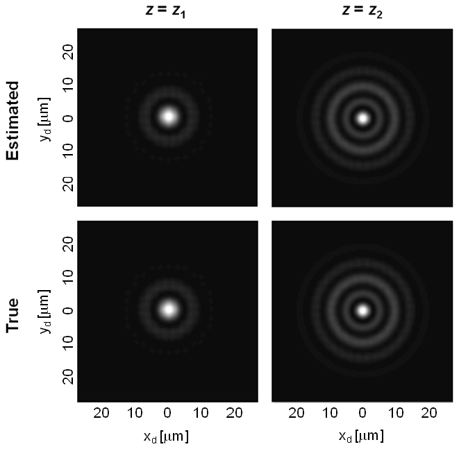
Comparison between the true and estimated irradiance patterns for the highly aberrated test lens.
Large deviations in the variance from the CRB may have arisen from the host of local extrema in the likelihood surface. If the magnitude of fluctuations is unacceptable in the specific application, then one must either devote more computation time to navigating the search space or find a system configuration with fewer extrema.
An iteration is defined as one cycle through every parameter, and there were 200 iterations, or 1.8 × 10³ forward propagations, per temperature phase. For the specified pupil sampling and FFT grid size, the computation time was 790 ms per forward propagation, which included both output planes. So, the average of 87.3 temperature phases per trial corresponds to 34.5 hours of computation time. We carried out this study using an NVIDIA Tesla C1060 GPU, whose peak double-precision (DP) performance is 78 GFLOPS. Had we used a Tesla C2075 model, offering 515 GFLOPS of DP power, the computation time per trial would have been roughly 5.2 hours. Further improvement can be achieved with a cluster of GPUs. For instance, the VSC455 V8 GPU workstation by Velocity Micro combines 8 Tesla C2075s for over 4 TFLOPS of DP power, which would turn the 5.2 hours into just 40 minutes. Another way to improve computational time involves beamlet-based propagation algorithms, such as CODE V Beam Synthesis Propagation (BSP), which can provide accurate and efficient modeling of the wave propagation.
7. Experimental results
7.1 System configuration
We obtained multifocal irradiance data in the focal region of a relatively benign spherical test lens at finite conjugates and with a HeNe source (λ = 0.6328 μm). The distance from the on-axis point source, created with a 40X microscope objective and 10-μm pinhole, to the test lens was 457 mm. To generate an increase in information by illuminating substantially more detector elements, we magnified the intermediate image with a relay lens placed just before the CCD. This had the added benefit of eliminating CCD saturation without the use of neutral density filters. The imaging lens was a Nikon 40X microscope objective (NA = 0.95), configured at the design conjugates. When used at the proper conjugates, the manufacturer claims the objective lens is corrected for spherical aberration. This particular objective was infinity-corrected with an optical tube length of 160 mm. To maintain these conjugates, we placed the imaging lens and CCD on a translation stage, allowing us to scan through the focal region of the test lens. We used a CCD with a fine pixel size of 4.4 μm for high information yield. In general, doubling the number of pixels also doubles the Fisher information, as indicated in Eq. (16), provided that the detector variance remains the same.
7.2 Test lens description
The test lens for this study was a double-convex spherical lens with a diameter of Dlens = 25 mm and radius of curvature of R1 = -R2 = 76.66 mm. According to ZEMAX, the exit pupil diameter and working f-number was Dxp = 25.39 mm and f/#w = 3.471, respectively. It was imperative that the image-space NA of the test lens (NA = 0.14) was less than that of the imaging lens to avoid information loss. The position of the paraxial focal plane was z = zf = 90.83 mm, where the z = 0 plane contained the exit pupil.
The ZEMAX calculations of the Fringe Zernike coefficients (N = 37) in the exit pupil of the lens are provided in Table 6 . With a smaller peak-to-valley wavefront error of 30.6λ, we anticipated less stringent requirements on the pupil sampling in our propagation algorithm. The minimum pupil sampling level was 256 × 256 for this lens, which we zero-padded for an FFT grid size of 1024 × 1024. This resulted in oversampling of the irradiance distribution, however, this only increased the computational time and did not affect the outcome of the study.
Table 6. Fringe Zernike coefficients {αn, n = 1,…, 37}, peak-to-valley, RMS, and variance, provided by ZEMAX for the highly aberrated test lens. Unlisted coefficients are zero.
| Index | Aberration Type [λ] | Design Value [λ] |
|---|---|---|
| 1
|
Piston
|
10.15431626
|
| 4
|
Defocus
|
15.26099035
|
| 9
|
Spherical Aberration, Primary
|
5.12576917
|
| 16
|
Spherical Aberration, Secondary
|
0.01863364
|
| 25
|
Spherical Aberration, Tertiary
|
−0.00048193
|
| 36
|
Spherical Aberration, Quaternary
|
−0.00002109
|
| 37
|
Spherical Aberration,
12th-order Term
|
−0.00000061
|
| Peak-to-valley [λ]
|
N/A
|
30.55920575
|
| RMS [λ]
|
N/A
|
8.99563403
|
| Variance [λ2] | N/A | 80.92143161 |
7.3 Irradiance data
Figure 7 displays the physical data that we used as input to our optimization algorithm, consisting of two image planes just before paraxial focus, where the scale bar corresponds to the intermediate image plane between the test lens and objective lens. In Section 7.6, we discuss the estimation of nuisance parameters in the system, namely, the exact image plane locations and the true magnification of the objective lens.
Fig. 7.
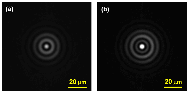
Experimental data for the spherical test lens for image planes: (a) z = z1 and (b) z = z2. Scale bar corresponds to the intermediate image plane just before the imaging lens.
7.4 Fisher information and Cramér-Rao bounds
We computed the FIM and its inverse (Fig. 8 ) for the Fringe Zernike coefficients to be estimated, {αn, n = 2,…, 9, 16}, based on the method in Section 6.3. The structure of these matrices is comparable to that for the highly aberrated lens, including strong coupling among the rotationally-symmetric terms, α4, α9, and α16. Since the CRB takes on diminutive values, the variance from detector noise is unlikely to preclude high-precision estimates.
Fig. 8.
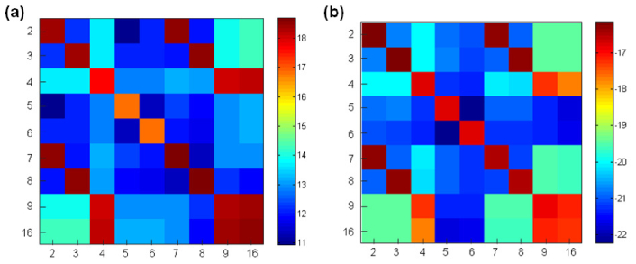
(a) FIM and (b) its inverse, for Fringe Zernike coefficients {αn, n = 2,…, 9, 16} in the exit pupil of the spherical test lens. Shown on a logarithmic scale.
Table 7. Square-root of the CRB for Fringe Zernike coefficients {αn, n = 2,…, 9, 16} in the exit pupil of the highly aberrated test lens at λ = 0.6328 μm. Units are in waves λ.
| Index | (CRB)1/2 [λ] | Index | (CRB)1/2 [λ] |
|---|---|---|---|
| 2
|
8.3 × 10⁻⁹
|
7
|
5.7 × 10⁻⁹
|
| 3
|
8.3 × 10⁻⁹
|
8
|
5.7 × 10⁻⁹
|
| 4
|
4.2 × 10⁻⁹
|
9
|
3.5 × 10⁻⁹
|
| 5
|
3.9 × 10⁻⁹
|
16
|
2.4 × 10⁻⁹
|
| 6 | 3.9 × 10⁻⁹ |
7.5 Nuisance parameters
Nuisance parameters are defined as parameters that affect the data and are therefore fundamental to the probability model, but are not useful to the estimation task. Suppose α denotes the wavefront parameters of interest, β denotes the wavefront parameters of no immediate interest, and χ denotes all other nuisance parameters, so that the entire vector parameter can be written as θ = (α, β, χ) t. Therefore, α is comprised of Zernike coefficients {αn, n = 2,…, 9, 16}, β is comprised of all remaining coefficients, and χ consists of unknown system parameters to be discussed next. We dealt with β by replacing it (up to the ZEMAX limit of N = 37) with the respective design coefficients in Table 6, denoted as β0, then separately estimated χ prior to the primary estimation task. Finally, we set and proceeded to estimate α.
Two of the critical nuisance parameters in the system were the absolute image-plane positions, z1 = zf + Δz1 and z2 = zf + Δz2. During acquisition of the detector data, it was difficult to accurately pinpoint the paraxial focal plane, z = zf, which served as the reference plane in our studies. Another nuisance parameter was the true magnification of the microscope objective just before the detector, denoted as M1 and M2 for the first and second image, respectively. To achieve the design magnification of 40X, the detector must be placed 160 mm from the rear principal plane of the objective lens, however, we had no knowledge of the exact location of this plane.
For the ith output plane, we estimated zi and Mi from the respective detector data in Fig. 7 by performing a straightforward 2D grid search. During this step, we fixed all wavefront parameters, α and β, to the design parameters, α0 and β0, and computed the cost function for both image planes assuming a Gaussian noise model (Fig. 9 ). Prior to generating these plots, we first did a broader search for local minima in the region of interest, but did not find any. The final nuisance parameter estimates were given by
| (19) |
| (20) |
where Δz is the distance from paraxial focus and M is the magnification.
Fig. 9.
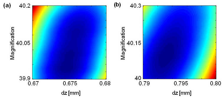
Determining the nuisance parameters in the system for image plane z = z2 via a 2D grid search prior to the estimation of wavefront parameters.
Since the detector element size was 4.4 μm, the effective pixel size after magnification was Δxd = 0.1101 μm and Δxd = 0.1098 μm. This resulted in sampling the irradiance distribution below the diffraction limit of approximately 0.5 λ/NA = 0.33 µm (i.e., oversampling by a factor of three). However, the excess magnification also allowed us to avoid detector saturation without the use of additional optics, as mentioned in Sec. 7.1.
7.6 Maximum-likelihood estimates
To compare the physical data with the output of the optical design program during optimization, we first interpolated the data, so that its coordinates matched that of the FFT output. Then we normalized the irradiance pattern in both the data and FFT output, which is analogous to normalizing the power of the source beam.
Using the method described in Section 6.5, we performed 12 estimation trials (Fig. 10 ). The starting point was based on the design values for the Zernike coefficients, since this offered the best possible initial guess, and a large parameter space was explored during the search (Table 8 ). The average final cost function was 0.150, while the average number of temperature phases was 105, corresponding to a temperature of 0.0174.
Fig. 10.
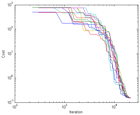
12 simulated annealing trials for the estimation of wavefront parameters in the exit pupil of the highly aberrated test lens, plotting the optimal cost function versus iteration number on a log-log scale.
Table 8. ML estimates of wavefront parameters for the spherical test lens at λ = 0.6328 μm, including their standard deviations. Design values were used as a starting point in the search. Ranges in the search space were relative to the design values. Units are in waves λ.
| Index | Design Value [λ] | Range | ML Estimate [λ] |
|---|---|---|---|
| 2
|
0
|
± 10λ
|
0.10 ± 0.30
|
| 3
|
0
|
± 10λ
|
−0.13 ± 0.28
|
| 4
|
15.26099035
|
± 20λ
|
15.57 ± 0.64
|
| 5
|
0
|
± 5λ
|
−0.09 ± 0.19
|
| 6
|
0
|
± 5λ
|
0.13 ± 0.26
|
| 7
|
0
|
± 5λ
|
0.08 ± 0.18
|
| 8
|
0
|
± 5λ
|
−0.11 ± 0.23
|
| 9
|
5.12576917
|
± 10λ
|
4.92 ± 0.32
|
| 16 | 0.01863364 | ± λ | 0.0196 ± 0.0014 |
Final average estimates and standard deviations for Zernike coefficients {αn, n = 2,…, 9, 16} are given in Table 8. Without knowledge of the true values or a gold standard, we have no basis for evaluating biases in the estimates, though the estimated values are within one standard deviation from the design values. Once again, large departures from the CRB may have resulted from the numerous local basins in the cost function.
There were 250 iterations or 2.25 × 10³ forward propagations in each temperature phase. For the given FFT grid size, the computation time was 308 ms per forward propagation. On average, there were 105 temperature phases per trial, corresponding to 20.2 hours of computation time with a single NVIDIA Tesla C1060. This amounts to 3.1 hours with a Tesla C2075 model, or 23.3 minutes with a VSC455 V8.
8. Conclusions
In both the numerical and experimental studies, the data-acquisition method involved multiple irradiance patterns collected near the focus of an optical system for the purpose of estimating the pupil phase distribution. We considered various approaches for a suitable propagation algorithm to accurately model the wave propagation and developed the mathematical framework for an aberrated wave emerging from the exit pupil, where we parameterized the wavefront using expansion functions, particularly, Fringe Zernike polynomials. To substantially reduce the computation time, we implemented parallel processing with a state-of-the-art GPU.
We obtained proof-of-principle results in both simulation and experiment. In each study, we evaluated the sampling requirements and verified that significant pupil sampling is needed for large wavefront errors. Fisher information matrices featured prominent coupling among specific groups of parameters, such as the group containing only rotationally-symmetric Zernike terms. The associated Cramér-Rao bounds were incredibly small, thereby permitting high-precision estimates, although this generally requires an accurate forward model and a search algorithm that can reliably locate the global minimum of the cost function.
After discovering numerous local extrema in the likelihood surfaces, we chose simulated annealing for the estimation of selected Zernike coefficients. In the numerical study with the highly aberrated lens, the estimate biases were negligible, probably because of the lack of systematic errors in the estimation procedure. Although the variances were fairly small, they were far from the CRB due to entrapment in local basins in the cost function.
In the experimental study, we used a benign test lens with significantly less aberrations and a larger working f-number of f/#w = 3.47. Since the imaging (i.e., relay) lens was much faster with f/# ≈0.53 (NA = 0.95), it should not have resulted in information loss from the suppression of high spatial frequencies. However, this may become an issue if the f-number of the test lens is low enough. To avoid having to include the imaging lens in the forward model here, one solution is to use the translation stage to place a ground glass in any plane where an irradiance measurement is desired, then relay the incoherent irradiance, instead of the field, to the detector. Note that it is necessary to have a rotating ground glass to decorrelate the resulting speckle noise. An alternative to a rotating diffuser is a liquid-crystal diffuser operated in a dynamic scattering mode.
Experimentally, we were challenged with the requirement of an accurate probability model, as well as the presence of nuisance parameters in the system. We verified the accuracy of the Fresnel approximation in our forward model compared to the Huygens wavelet formula. Nuisance parameters included image plane positions and the true magnification of the imaging lens. We dealt with them by means of a 2D grid search and located a single extremum for each image plane. The estimate variances were comparable to those in the simulation study, and each estimate did not exceed one standard deviation compared to the design values.
Acknowledgments
This work was supported by Canon, Inc. and the National Institutes of Health under grant number R37 EB000803. We would also like to thank Jin Park, Luca Caucci, and Akinori Ohkubo for their valuable input.
References and links
- 1.Stefanescu I. S., “On the phase retrieval problem in two dimensions,” J. Math. Phys. 26(9), 2141–2160 (1985). 10.1063/1.526837 [DOI] [Google Scholar]
- 2.Seldin J. H., Fienup J. R., “Numerical investigation of the uniqueness of phase retrieval,” J. Opt. Soc. Am. A 7(3), 412–427 (1990). 10.1364/JOSAA.7.000412 [DOI] [Google Scholar]
- 3.Teague M. R., “Deterministic phase retrieval: a Green’s function solution,” J. Opt. Soc. Am. 73(11), 1434–1441 (1983). 10.1364/JOSA.73.001434 [DOI] [Google Scholar]
- 4.G. R. Brady and J. R. Fienup, “Improved optical metrology using phase retrieval,” 2004 Optical Fabrication & Testing Topical Meeting, OSA, Rochester, NY, paper OTuB3 (2004). [Google Scholar]
- 5.Brady G. R., Fienup J., “Phase retrieval as an optical metrology tool,” Optifab: Technical Digest, SPIE Technical Digest TD03, 139–141 (2005). [Google Scholar]
- 6.Brady G. R., Guizar-Sicairos M., Fienup J. R., “Optical wavefront measurement using phase retrieval with transverse translation diversity,” Opt. Express 17(2), 624–639 (2009). 10.1364/OE.17.000624 [DOI] [PubMed] [Google Scholar]
- 7.H. H. Barrett and K. J. Myers, Foundations of Image Science (Wiley, 2004). [Google Scholar]
- 8.J. W. Goodman, Introduction to Fourier Optics (Roberts & Company Publishers, 2005). [Google Scholar]
- 9.Corana A., Marchesi M., Martini C., Ridella S., “Minimizing multimodal functions of continuous variable with the ‘simulated annealing’ algorithm,” ACM Trans. Math. Softw. 13(3), 262–280 (1987). 10.1145/29380.29864 [DOI] [Google Scholar]
- 10.Barrett H. H., Dainty C., Lara D., “Maximum-likelihood methods in wavefront sensing: stochastic models and likelihood functions,” J. Opt. Soc. Am. A 24(2), 391–414 (2007). 10.1364/JOSAA.24.000391 [DOI] [PMC free article] [PubMed] [Google Scholar]
- 11.Rao C. R., “Information and accuracy attainable in the estimation of statistical parameters,” Bull. Calcutta Math. Soc. 37, 81–91 (1945). [Google Scholar]
- 12.H. Cramér, Mathematical Methods of Statistics (Princeton University Press, 1946). [Google Scholar]


