A simple model of mechanotransduction in primate glabrous skin

Abstract

Tactile stimulation of the hand evokes highly precise and repeatable patterns of activity in mechanoreceptive afferents; the strength (i.e., firing rate) and timing of these responses have been shown to convey stimulus information. To achieve an understanding of the mechanisms underlying the representation of tactile stimuli in the nerve, we developed a two-stage computational model consisting of a nonlinear mechanical transduction stage followed by a generalized integrate-and-fire mechanism. The model improves upon a recently published counterpart in two important ways. First, complexity is dramatically reduced (at least one order of magnitude fewer parameters). Second, the model comprises a saturating nonlinearity and therefore can be applied to a much wider range of stimuli. We show that both the rate and timing of afferent responses are predicted with remarkable precision and that observed adaptation patterns and threshold behavior are well captured. We conclude that the responses of mechanoreceptive afferents can be understood using a very parsimonious mechanistic model, which can then be used to accurately simulate the responses of afferent populations.

all perception starts with the activation of peripheral sensors that communicate information about the outside world to the central nervous system. A careful characterization of their information transmission properties is therefore crucial for understanding subsequent processing and also of practical relevance for haptics and neuroprosthetics.

In the primate somatosensory system, information about cutaneous stimulation is conveyed by four classes of low-threshold mechanoreceptive afferents, of which three classes exist in the macaque hand: slowly adapting type 1 (SA1, in the following referred to as SA), rapidly adapting (RA), and Pacinian (PC) afferents (Johnson 2001) [we are not concerned with SA2 mechanoreceptors, which are absent from the glabrous skin of the macaque hand (Pare et al. 2002)]. SA afferents, originating in Merkel cells in the skin, convey information about the shape of objects grasped in the hand; RA afferents, which innervate Meissner corpuscles, are involved in motion detection and grip control; and PC afferents, which innervate Pacinian corpuscles, are highly sensitive to high-frequency skin deformations.

Mechanoreceptive afferents produce highly repeatable responses to complex skin vibrations (Looft 1996; Muniak et al. 2007) and the details of spike timing conveying information about stimulus features (Johansson and Birznieks 2004; Mackevicius et al. 2012; Saal et al. 2009). For example, complex skin vibrations, such as those experienced during texture scanning, can be classified based on the temporal spiking patterns they evoke and millisecond-precision spike timing shapes the way these vibrations are perceived (Mackevicius et al. 2012). Models of mechanotransduction should thus capture neuronal firing patterns at high temporal precision. Bensmaia (2002) showed that an integrate-and-fire model using input from skin indentation and its temporal derivative, velocity, reproduce the mean firing rates of RA fibers. Kim et al. (2010) expanded this approach to all three classes of somatosensory afferents. Their model comprises a linear prefilter and a standard integrate-and-fire model, with its parameters determined using maximum likelihood methods (Paninski et al. 2004). The model reproduces not only mean firing rates but also precise spike times. The model has, however, two important limitations. First, the transduction element of the model comprises hundreds of parameters (a minimum of 129 for the simplest version and a maximum of 969 for the most complex) making it very difficult to optimize and use. In light of this, we develop a more parsimonious model that achieves at least comparable performance with a minimal number of free parameters. Second, the original model cannot account for response saturation. While firing rates of SA neurons increase rather linearly with stimulus amplitude over a wide range of amplitudes, and RA and PC responses exhibit saturation even at moderate amplitudes (Kim et al. 2010; Vega-Bermudez and Johnson 1999). Introducing saturation makes it difficult to optimize model parameters because the optimization depends on the concavity of the log-normal likelihood function, a condition not fulfilled if the model is nonlinear (Paninski et al. 2004). Without this property, adjusting the hundreds of free parameters is virtually impossible. With this in mind, we introduce a novel optimization method that can accommodate response nonlinearities such as saturation.

MATERIALS AND METHODS

The detailed experimental methods and stimulus descriptions have been described (Kim et al. 2010; Muniak et al. 2007). We briefly summarize them here.

Neurophysiology

All experimental protocols were approved by the Johns Hopkins University Animal Care and Use Committee and complied with the guidelines of the National Institutes of Health Guide for the Care and Use of Laboratory Animals. Single unit recordings were performed in the ulnar and median nerves of two anesthetized Macaque monkeys (Macaca mulatta) by standard methods (Talbot et al. 1968). Mechanoreceptive afferent fibers were classified according to their responses to step indentations and vibratory stimulation (Freeman and Johnson 1982; Talbot et al. 1968). An afferent fiber was classified as slowly adapting if it produced sustained firing in response to a step indentation. The neuron was considered rapidly adapting if it had a small receptive field and responded only to the onset and offset of an indentation. Pacinian corpuscles were identified as afferents that were vigorously activated by air blown gently over the hand, activated by transmitted vibrations produced by tapping on the hand restraint, and if they had large receptive fields. In all cases, the hotspot of the receptive field was located on the skin using a handheld probe and then marked with a felt tip pen. The stimulator probe was centered on the hotspot to the extent possible, and the tip of the probe was then glued to the skin with cyanoacrylate at its resting position, i.e., with no preindentation. Note that gluing the probe to the skin has little effect on the perception of these vibrations (Muniak et al. 2007).

Apparatus

A custom-made motor (Chubbuck 1966) was used to deliver tactile stimuli. It was driven by a servo-controlled amplifier and equipped with a high-precision linear variable displacement transducer with submicron resolution. The input voltage to the amplifier was generated under computer control using a digital to analog card (PCI-6229; National Instruments, Austin, TX: output rate = 20 kHz). The displacement sensor was calibrated using an Optodyne laser interferometer (Optodyne LDS 1000, Compton, CA), which is capable of measuring absolute displacement to submicron resolution. The actual position, as measured by the interferometer, was regressed onto the output of the position sensor. The contactor consisted of a steel-tipped stylus fixed to the table of the Chubbuck motor. The stylus was 175-mm long with a radius of 12.5 mm and a weight of 12.5 g. The tip of the stylus was flat and had a diameter of 1 mm (Freeman and Johnson 1982).

Stimuli

Sinusoids.

Sinusoids (sine waves) were presented at 1, 5, 10, 25, 60, and 100 Hz. At 1 Hz, amplitudes ranged from 5 to 360 μm, zero-to-peak; at 5 Hz, 1–180 μm; at 10 Hz, 2.5–130 μm; at 25 Hz, 0.4–10 μm; at 60 Hz, 0.1–170 μm; and at 100 Hz, 0.5–130 μm. The stimulus duration was either five stimulus cycles or 0.1 s, whichever was longer. At each frequency, amplitudes were incremented in equal logarithmic steps over the range. The interstimulus interval was 0.1 s. In total, 120 different sinusoids were presented.

Diharmonic stimuli.

Diharmonic stimuli were sums of two sine waves, as follows,

$$x\left(t\right)=A_1\sin \left({\omega }_{1}t\right)+A_2\sin \left({\omega }_{2}t+\phi \right)$$ (1)

where A₁ and A₂ are the amplitudes of the low- and high-frequency components, respectively, ω₁ and ω₂ are the two frequencies (ω₁ < ω₂), and ϕ is the phase of the high frequency component relative to that of the low-frequency component. Component amplitudes ranged from 2 to 125 μm if their frequency was <100 Hz and from 2 to 100 μm at 100 and 125 Hz. The phase ϕ took on one of four values: 0, π/2, π, or 3π/2. The stimulus duration was either five cycles of the low-frequency component or 0.1 s, whichever was longer. The amplitudes of the two frequency components were incremented in equal logarithmic steps over their respective ranges. The interstimulus interval was 0.1 s. In total, 240 different diharmonic stimuli were presented.

Band-pass noise stimuli.

Wide-band noise was band-pass filtered to the specified frequency range using a finite impulse response filter (the fir1 function, MATLAB; The Mathworks, Natick MA). The low cut-off frequency was 5 Hz, and the high cut-off frequencies were 10, 25, 50, and 100 Hz. Each noise stimulus was scaled to a set of predetermined root-mean-square amplitudes, namely 0.5, 1, 5, 10, and 50 μm. The duration of all noise stimuli was 1 s. Each stimulus was preceded and followed by a 1-s interstimulus period with no stimulation to reduce the effects of vibratory adaptation (Bensmaia et al. 2005; Leung et al. 2005). In total, 20 different noise stimuli were presented.

Neuron Selection

Unlike most cortical neurons, peripheral afferents typically produce highly reliable and reproducible responses to strong stimuli. In light of this, we sought to identify neurons with excessive variability, or whose excitability drifted over time, and to exclude them from further analysis. From the set of all 25 neurons that were successfully recorded for all sine (120 conditions), diharmonic (240 conditions), and noise (20 conditions) stimuli with five repetitions each, we rejected neurons with large variations in firing rate across repetitions, or with high baseline firing rates because we considered them to be unreliable. These two exclusion criteria were defined as follows.

We first determined whether a given stimulus was sufficiently intense to evoke reliable responses. Each stimulus was presented five times to each neuron. If less than two spikes were evoked on any presentation, we concluded that the stimulus was perithreshold, that is, close to this neuron's threshold (recall that each repetition comprised at least 5 complete cycles of a sinusoid, or of the low-frequency component, of a diharmonic stimulus). As high variability is expected to occur for all perithreshold responses, data from all repetitions with near-threshold stimuli were not taken into account when making the decision whether a given neuron was considered too unreliable. For the remaining (supra threshold) stimulus conditions, we computed the Fano factor, i.e., the ratio of the variance to the mean of the spike count. If the Fano factor averaged over all stimulus conditions exceeded 0.2, we considered the neuron as too noisy and it was rejected from further analysis.

The second exclusion criterion was designed to reject neurons with high baseline firing rates. Most mechanoreceptive afferents have very low spontaneous activity; therefore, we excluded neurons whose baseline firing rate exceeded 0.2 spikes per second. Application of our selection criteria resulted in the exclusion of 3 neurons, leaving 5 SA, 14 RA, and 3 PC fibers for further analysis.

Integrate-and-Fire Model

We develop a model of neuronal firing consisting of two parts. The first is a transduction model, which converts the mechanical signal into a set of electrical currents. The sum of these currents constitutes the input to the second part, which generates the spike sequence.

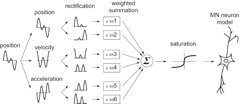
The transduction model is shown in Fig. 1. Kim et al. (2010) showed that the major contributions result from the displacement and its first and second (but not third) derivatives and that these contributions differ across afferent classes. Thus velocity and acceleration are computed numerically from the recorded displacement by a second order finite difference method. The numerical differentiation process introduces spurious frequency components >300 Hz, which are removed by a low pass filter. Displacement, velocity, and acceleration are then each split into their positive and negative components, and each of these rectified components enters as an independent signal (Fig. 1). We use the symbol s for the weighted sum of these six signals, with the weights ω₁, …, ω₆ being free parameters of the model.

Fig. 1.

Mechanotransduction model. The displacement x is the input to the transduction model. Velocity and acceleration are computed by numerical differentiation. Each of the 3 mechanical signals is split into positive and negative components that are rectified and multiplied by a separate weight ω_i, and the resulting 6 signals are summed. A saturation filter is applied to the weighted sum. The output of the saturation filter, parametrized by I₀, is the input current for the generalized integrate-and-fire model (MN Neuron; Mihalas and Niebur 2009).

To model saturation effects, a one-parameter saturation filter S(s) is applied to the weighted sum s, with S(s) defined by

$$S\left(s\right)=\frac{I_{0}s}{I_0+\left|s\right|}$$ (2)

where I₀ is a free parameter. Note that the saturation effect decreases with increasing I₀. There is thus of a total seven parameters (ω₁, …, ω₆, I₀) for the transduction model. For comparison, each weight parameter replaces a filter comprising tens if not hundreds of parameters in the previous model (Kim et al. 2010). The only new parameter is I₀, the saturation parameter.

The output of the saturation filter constitutes the input, I(t), to a neuronal model which in turn generates a spike train based on this input current and its internal dynamics. We use a generalized integrate-and-fire model (Mihalas and Niebur 2009) with two dynamic variables, the membrane voltage V(t) and an adaptive threshold Θ(t). They are governed by the following equations,

$$V\prime \left(t\right)=-\frac{1}{\tau }\left[V\left(t\right)-V_{rest}\right]+\frac{I\left(t\right)+I_{ind}\left(t\right)}{C}$$ (3)

$$\Theta \prime \left(t\right)=a\left[V\left(t\right)-V_{rest}\right]-b\left[\Theta \left(t\right)-{\Theta }_{\infty }\right]$$ (4)

where C = 150 pF, V_rest = −70 mV, Θ_∞ = −30 mV, and b = 10 s⁻¹ are fixed constants representing, respectively, capacitance, resting membrane potential, equilibrium threshold, and inverse threshold rebound time constant of the model neuron. Free parameters include the threshold adaptation time constant, a, and the membrane time constant τ. Since the membrane time constant is equal to the product of capacitance and resting (or leakage) resistance and we consider the capacitance as a fixed parameter defined by the size and geometry of the cell, variation of the time constant is equivalent to variation of the resting resistance. The adaptive threshold, Θ(t), allows the model to incorporate the known effects of adaptation on afferent excitability. Indeed, prolonged suprathreshold stimulation causes a decrease in afferent sensitivity, a decrease that is associated with increases in spiking threshold (Bensmaia et al. 2005; Leung et al. 2005).

The model also comprises a spike-induced current I_ind(t), resulting from two types of ion channels (i₀ and i₁). One has a short decay time constant, τ₀ = 5 ms, to mimic relative refractoriness, and the other has a longer decay time constant τ₁ = 50 ms to mimic spike-induced currents that operate at longer time scales. The inclusion of two spike-induced currents at different time scales allows the model to exhibit a large number of observable spiking behaviors (e.g., burstiness) and provided better fits than did inclusion of a single one. Mathematically, I_ind is expressed as:

$$\begin{array}{c}{I}_{ind}=i_0+i_1\\ i{\prime }_0=-i_0/{\tau }_0\\ i{\prime }_1=-i_1/{\tau }_1\end{array}$$ (5)

A spike is generated when V(t) = Θ(t). Then the membrane voltage is reset to V_rest and the threshold is reset to max[Θ(t), Θ_∞]. The spike induced currents are added to the two channels:

$$\begin{array}{c}{i}_0\leftarrow i_0+A_0\\ i_1\leftarrow i_1+A_1\end{array}$$ (6)

where A₀ and A₁ are the amplitudes of the currents resulting from the two types of ion channels. These two amplitudes are additional free parameters of the model.

In total, there are thus four free parameters in the spike-generation model: τ, a, A₀, and A₁. There is one additional free parameter which is the transduction delay between the time when the tactile stimulus is applied to the skin and when the action potential is recorded by the electrode in the nerve. In summary, our model has a total of 12 free parameters: 7 for the transduction model, 4 for the spike generation, and 1 for the transduction delay.

We anticipated that differences across afferent types would be captured in the degree to which indentation depth and its two derivatives would drive the responses, in the degree to which these quantities were rectified, and in the biophysical properties of the neurons, as reflected in the parameters of the integrate-and-fire model.

Model Optimization

For the purposes of optimization, the model prediction of each spike time is based on the previous spike produced by the afferent, not that produced by the model. That is, the model only predicts one spike in the future based on the actual history of the neuron. Model parameters are determined by minimizing a cost function. A natural choice for the cost function is the likelihood function of the model generating the observed spike train given the input signal (Dong et al. 2011a,b; Paninski et al. 2004; Russell et al. 2010). In practice, however, the evaluation of the likelihood function is computationally demanding and it is not feasible to evaluate the likelihood function for the large neuronal data sets used in this study. Instead, we use a more efficient cost function that minimizes the difference between observed and model-generated spike time intervals (Dong et al. 2011b), which we summarize now shortly. A spike train can be described as the ordered set of intervals between consecutive spikes. Suppose that the length of the ith observed spike time interval is Tⁱ and that T_mⁱ is the corresponding model-generated interval. We define the cost function for this spike time interval as Fⁱ,

$$F^i=1-e^{-\log {\left(T_m^i/T^i\right)}^2}$$ (7)

The choice of this cost function is based on the assumption that variations in the interspike-intervals are approximately log-normally distributed (note that we do not make an assumption on the means of interspike-interval distributions, only on their variations) (Dong 2010). The log-normal distribution is frequently found for stochastic variables whose mean values are low with their variances large and whose values cannot be negative (Limpert et al. 2001), all characteristics typically encountered in interspike interval distributions. Indeed, log-normal distributions have been found in many neuronal systems, both in vivo and in vitro, e.g., (Bershadskii 2001; Beyer et al. 1975; Burns and Webb 1976; Levine 1991; Webb 1976a, b). For small differences between the interspike intervals, the cost function in Eq. 7 approaches the negative log-likelihood function of the lognormal distribution (Dong et al. 2011b). Note, however, that while these arguments provide a motivation for the choice of Eq. 7 as a cost function, we emphasize that the ultimate justification for this choice is in the quality of the predictions generated by the model, optimized using the cost function. These predictions will be tested below.

The total cost function is defined as

$$F={\displaystyle \sum _i{F}^i}$$ (8)

where the sum runs over all intervals except those deemed outliers (see below for criterion). To minimize F as a function of the 12 free parameters of our model, we use an optimization algorithm that combines evolutionary techniques with optimization on a simplex (Efstratiadis and Koutsoyiannis 2002). The procedure starts with a large population (300) of vertices (starting values for each parameter) out of which a simplex is formed by random selection. The Nelder-Mead algorithm is then combined with evolutionary techniques (mutations and crossings) and run on this simplex (see Efstratiadis and Koutsoyiannis 2002 for details). To account for the possibility that neuronal noise results in some interspike intervals with uncharacteristically poor fit (outliers), we designed a two-stage optimization procedure, with outliers being identified in the first stage and eliminated in the second. In the first stage, we compute the sum on the right-hand side of Eq. 8, excluding the m% of intervals with the highest cost. If high-cost intervals are not excluded, fitting procedures are sometimes dominated by these intervals, and the optimization algorithm slows down and sometimes cannot find the optimal solution. We ran 21 independent optimizations, 1 each for the 21 values of m (ranging from 0 to 20). In the second stage, we used the results of the first stage and computed the model fit (using the Γ factor, as described below) for each of the 21 results of the first stage. We then selected that parameter set that gave the best fit across all values of m.

Quantifying Spike Train Dissimilarity

To evaluate how well the model-generated spike trains match the experimental spike trains, we use two complementary measures. One is a global (coarse) measure, which is simply the mean firing rate in a trial or, equivalently, the number of action potentials per trial. Distance between sets of spike trains is then quantified as the Pearson correlation coefficients of the firing rates computed from the set of all trials.

To gauge differences in the fine temporal structure of the spike trains, we use a second measure that is based on the rate of coincidences within a fixed window (±4 ms in this study) relative to the number of coincidences expected in this interval for two independent spike trains with Poisson statistics (other spike-distance measures have been proposed, e.g., van Rossum 2001; Vega-Bermudez and Johnson 1999). This benchmark, proposed by Kistler et al. (1997) and adopted by the Quantitative Single-Neuron Modeling 2009 competition of the International Neuroinformatics Coordination Facility, is usually called the “Γ-factor” (Jolivet et al. 2008). A perfect match of two spike trains results in Γ = 1, two spike trains that do not have more coincidences than expected by chance for Poisson statistics have Γ = 0, and Γ < 0 is a sign of anticorrelation. Note that we assume Poisson statistics here rather than the lognormal statistics that we used to motivate the choice of the cost function. We do this both for simplicity and because we want to stay consistent with the standard definition of the Γ-factor by Jolivet et al. (2008). To take into account the intrinsic neuronal variability across repetitions, we define a variable R as the mean Γ-factor between pairs of observed spike trains. The Γ performance of the model, Γ_n, is then defined as the average Γ-factor between model and observed spike trains and divided by R,

$${\Gamma }_{\text{n}}=\frac{\overline{{\Gamma }_j}}{R}$$ (9)

where Γ_j measures the dissimilarity between the jth measured spike train and the model spike train (note that we follow the INCF Quantitative Single-Neuron Modeling 2009 competition, see equation defining P_A in http://www.incf.org/Events/competitions/spike-time-prediction/2009/InstructionForParticipants2009.pdf). If Γ_n equals unity, the model spike train is as close to the observed spike train as the latter is to any other observed spike train.

While the predictions were generated using a noise-free model, the small amount of variability in afferent spiking can be readily incorporated by including a noise term to the expression for the input current [I(t) in Eq. 3] (cf. Kim et al. 2010).

RESULTS

We fit the model to the responses of 22 afferents (5 SA, 14 RA, and 3 PC) and assessed 1) the accuracy with which the model could account for afferent responses, 2) how the model's performance compared with that of its predecessor, 3) how its parameters differed across afferent classes, and 4) whether it captured some of the key properties of mechanoreceptive afferent responses. An important point of emphasis was to determine whether the model could accurately reproduce not only afferent firing rates but also the precise timing of afferent responses, given its demonstrated importance (Johansson and Birznieks 2004; Mackevicius et al. 2012; Saal et al. 2009).

We separated the data sets into a training and a test set. Responses evoked by sinusoidal and diharmonic stimuli formed the training set and were used to train the model. The trained model was then used to generate spike trains in response to band-pass filtered noise, and the model performance was assessed by comparing the model-generated spike trains with the observed ones.

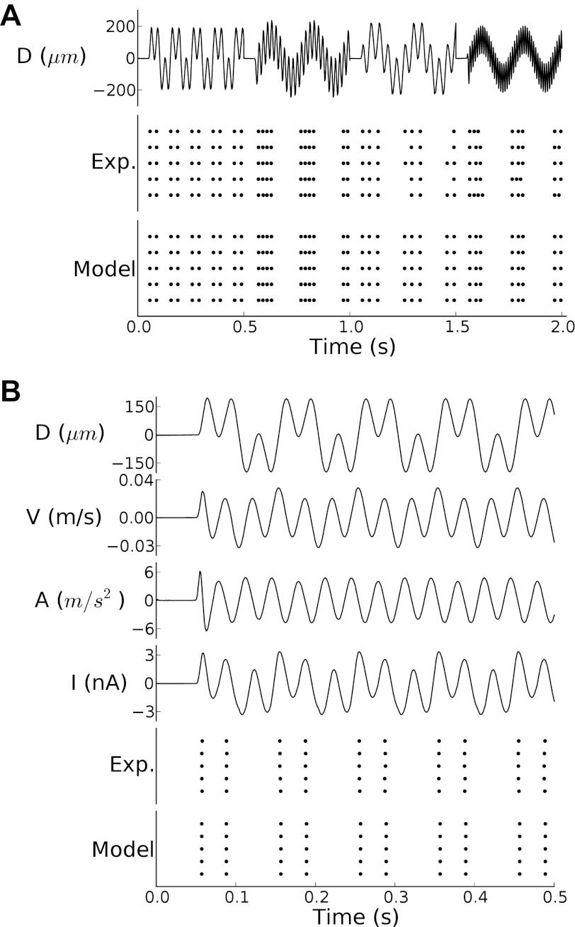
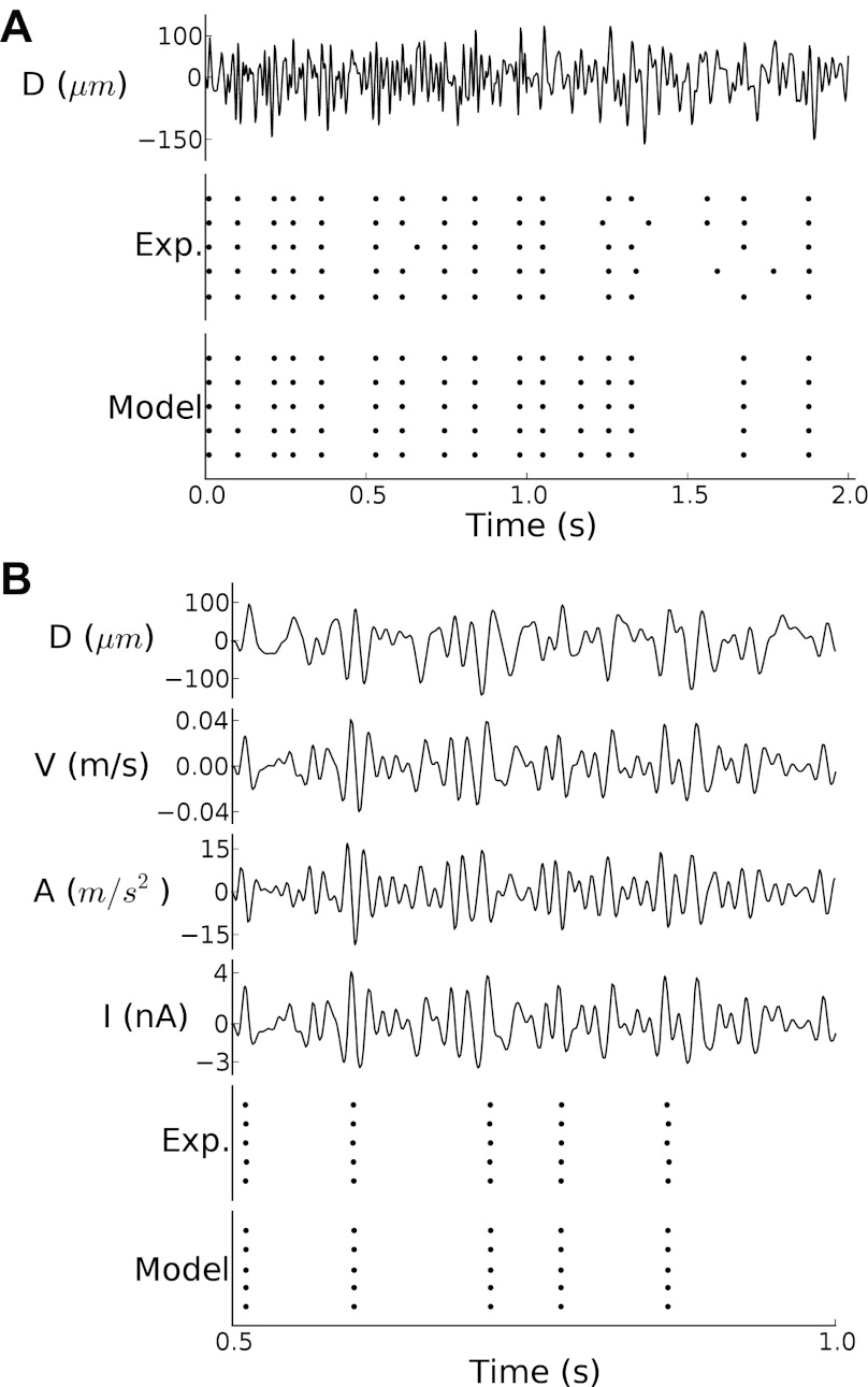
As shown in Figs. 2 and 3 for an example SA afferent, the model accurately predicted the responses to both sinusoids and noise stimuli, despite the fact that it had never been exposed to the latter. The model was able to accurately predict the responses to the training and test sets, as evidenced by the fact that the correlations between the measured and predicted firing rate were 0.986 and 0.992 for the two data sets, respectively. The model was also able to accurately capture the precise timing in the response, yielding values of Γ_n of 0.98 and 1 for the training and test sets, respectively.

Fig. 2.

Responses of a typical SA neuron to four diharmonic stimuli from the training set along with model predictions. A, top, displacement signal; center, observed spikes; bottom, model-generated spikes. The frequency pairs of the 4 diharmonic stimuli are (10,30), (5,50), (5,25), and (5,100) Hz, and their phase differences are 0, 180, 180, and 270°. The performance of the model, as gauged by Γ_n, was 1, 1, 0.92, and 1 for the 4 stimuli. B: first stimulus of A, shown at a finer scale. From top to bottom: mechanical displacement, velocity, acceleration, input current after adaption filter, observed spikes, and model-generated spikes.

Fig. 3.

Responses to a noise stimulus from the test set along with model predictions. Conventions for A and B are as in Fig. 2.

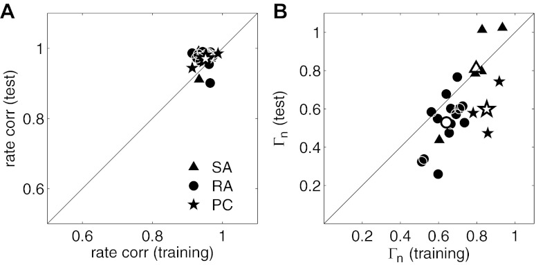
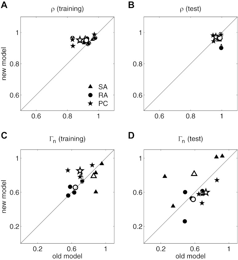
Model performance was high across the entire population as evidenced by rate correlation coefficients >0.9 for all 22 afferents for both data sets and values of Γ_n >0.5 for the training set. Overall, SA models performed better than RA or PC models (both in training and prediction; Fig. 4B). On the test set, one SA, one PC and 4 RA models yielded values of Γ_n <0.5.

Fig. 4.

Model performance for the 22 neurons. Rate correlation coefficients (A) and Γ_n (B) for the test and training sets. Triangles, circles, and stars denote slowly adapting (SA), rapidly adapting (RA), and Pacinian (PC) neurons, respectively. The mean for each neuron type is indicated by open symbols of the corresponding shape.

Next, we compared the performance of the new model to that of the old, parameter-heavy model (Kim et al. 2010). We found that the new model performed slightly better than the old model in predicting afferent firing rates (Fig. 5, A and B), a difference that was significant for the training set [t(11) = 2.87, P < 0.05] but not the test set [t(11) = 1.88, P < 0.08]. This slight increment in performance likely reflects the fact that the new model allows for response saturation whereas the old model does not (note that few high-amplitude stimuli were used in this comparison; see below for more detailed analysis of the impact of the saturation parameter I₀). The two models performed equally well in predicting spike timing (exact test, P = 0.38 and 0.77 for the training and test sets, respectively; Fig. 5, C and D). Thus the simple model presented here accounts for the strength (firing rate) and timing of afferent responses as well as or better than a more complex model requiring orders of magnitude more parameters.

Fig. 5.

Comparison of predictions of the present model (“new model”) with those of the model by Kim et al. (2010) (“old model”). A and B: rate correlation coefficients for the training and test sets, respectively. C and D: Γ_n for the training and test sets, respectively.

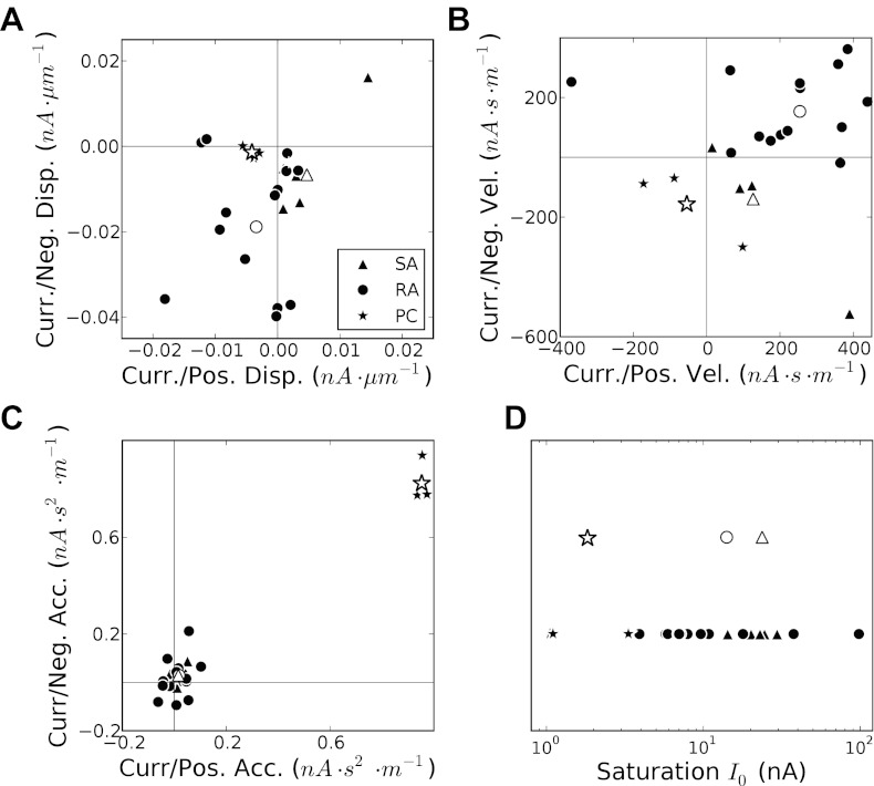
One of the conclusions of the previous study (Kim et al. 2010) was that different types of afferent neurons transduce different aspects of skin deformation: SA fibers are sensitive to displacement (depth of indentation) and velocity (rate of change of the depth), RA fibers to velocity alone, and PC fibers to displacement, velocity, and acceleration. One consequence of this differential pattern of sensitivity is that models of the different afferent types comprise different numbers of parameters. In the current model, the simplified transduction model allows us to use a unified framework with all three mechanical signals included for all neuron types. Each neuron is fitted with the same 12 free parameters. We can then compare the values of these parameters across afferents to infer differences in their properties. SA neurons are primarily driven by displacement and rectify their input as evidenced by the fact that they tend to cluster in the lower right quadrant (Fig. 6A). RA neurons are driven primarily by full-wave-rectified velocity (Fig. 6B). Acceleration only makes a small contribution to RA and SA neurons but it influences PC neurons strongly, and does so after rectification (Fig. 6C).

Fig. 6.

Fitted transduction parameters for all neurons (A–D). Closed symbols denote parameters obtained from individual neurons, and open symbols denote the means for each afferent type. In D, means are displaced vertically for clarity.

As expected and shown in Fig. 6D, PC afferents exhibit the strongest saturation effects (small values of I₀), followed by RA then SA neurons.

Effects of Stimulus Amplitude and Saturation

Mechanoreceptive afferent responses vary with the amplitude of vibratory stimuli in a characteristic way (Freeman and Johnson 1982; Johnson 1974). For weak periodic stimuli, firing frequency increases linearly with stimulus amplitude since a spike is elicited for a larger and larger fraction of vibration cycles until the neuron fires once on every cycle. Further increases of the amplitude only advance the phase of the spike within the cycle but do not increase the firing rate. Then, at substantially higher intensity levels, more than one spike is generated per cycle until the next plateau is reached at two spikes per cycle. Thus the firing rate of somatosensory afferents varies with increasing stimulus amplitude in a characteristic staircase sequence of plateaus.

Figure 7 shows the number of spikes per vibration cycle for two different stimulus frequencies (20 and 40 Hz) as a function of the stimulation amplitude in the range 1 to 250 μm. In all cases, the model accurately captures the rate intensity functions for both individual neurons (Fig. 7, A, C, and E) and afferent populations (Fig. 7, B, D, and F).

Fig. 7.

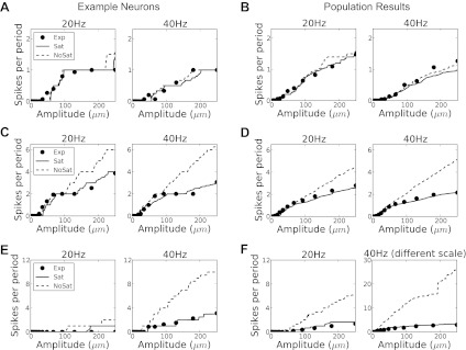
Rate intensity functions. Dots denote observed rates, solid lines, rates predicted using the full model, and dashed lines, predicted rates without saturation. A and B: SA neurons. C and D: RA neurons. E and F: PC neurons. A, C, and E: responses of representative individual neurons and the corresponding model predictions; B, D, and F: means over all neurons in each afferent category. Note the different scales of the ordinates in F.

As was emphasized by Kim et al. (2010), the linearity of their model precluded their model from capturing response saturation at higher stimulus amplitudes. To assess contribution of the saturation term, we solved the model equations with the saturation term removed and generated firing rate predictions. We found that the saturation term had only a moderate impact on the predictions of SA responses but a dramatic one on the predictions of both RA and PC responses, as might be expected given the magnitude of the saturation parameter I₀, which was lowest for PC neurons and highest for SA neurons. Saturation exerted a stronger influence on the response to high-frequency (40 Hz) than low-frequency (20 Hz) stimuli, particularly for neuron types that were sensitive to velocity and acceleration (RA and PC); this is expected since contributions from velocity increase linearly with frequency and those from acceleration quadratically. We conclude that saturation plays an important role in shaping afferent responses and that our model accurately captures this response property.

Absolute and Entrainment Thresholds

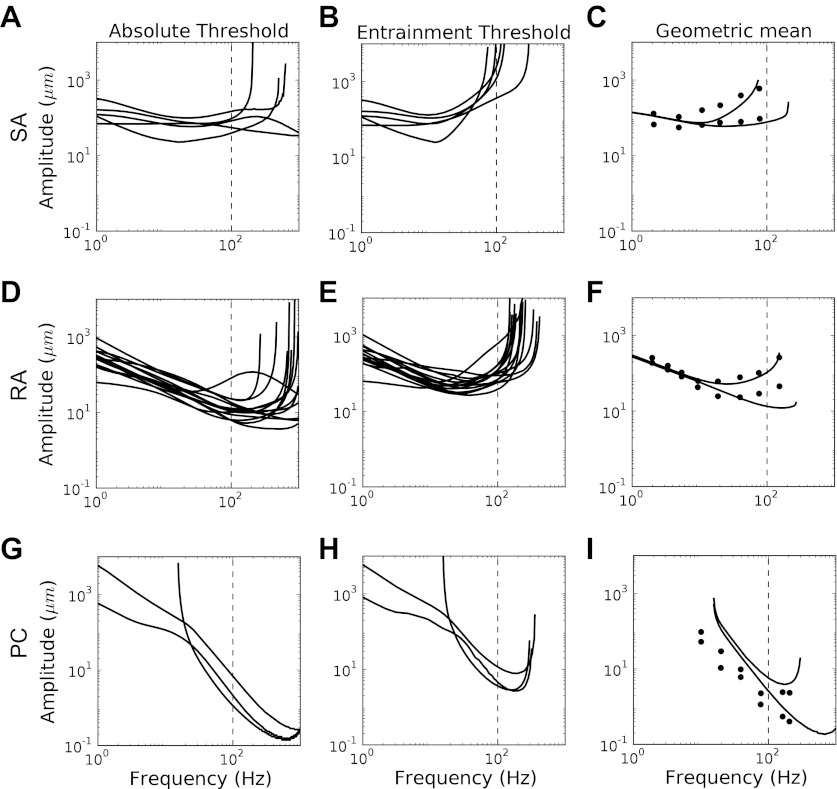
One classical measure of neuronal behavior is the firing threshold as a function of stimulus intensity. In the case of vibrotactile stimuli, this threshold is highly frequency dependent. Two measures of sensitivity to sinusoidal vibrations have been traditionally used (Johnson 1974; Muniak et al. 2007): the absolute threshold and the entrainment threshold. The absolute threshold is the lowest amplitude at which a spike is elicited with some (criterion) degree of reliability. We defined the absolute threshold as the minimal stimulus amplitude that causes the neuron to fire an average of one spike every fifth cycle. The entrainment threshold is the minimum amplitude that results in one spike per cycle on average. To obtain thresholds from our models, we simulated responses to sinusoids with frequencies ranging from 1 to 1,000 Hz for 100 cycles. Amplitudes were varied (by bisection) to determine the absolute and entrainment thresholds of each model neuron at each frequency. As shown in Fig. 8, model thresholds match previously measured thresholds for all three afferent types (Freeman and Johnson 1982). The match between simulated and measured thresholds is all the more remarkable given that model parameters were obtained 1) from the supraliminal behavior of neurons (stimuli in the training set were considerably above threshold), and 2) over a much narrower range of frequencies (up to 100 Hz, a tenth of the prediction range). Thus the threshold behavior of the model reflects considerable extrapolation over amplitude and frequency.

Fig. 8.

Firing thresholds for SA (A–C), RA (D–F), and PC (G–I) fibers. Shown are absolute (A, D, and G) and entrainment (B, E, and H) thresholds for the neurons individually. In C, F, and I, the lines denote the geometric means of the absolute (bottom) and entrainment (top) thresholds. Experimental data, shown as dots, were obtained from Freeman and Johnson (1982).

DISCUSSION

In the present study, we introduce a simple model that accounts for most of the known properties of mechanoreceptive responses to vibratory stimuli. We show that this model captures both the strength (mean firing rates) of the responses of mechanoreceptive afferents and their timing. Consistent with previous studies (Bensmaia 2002; Kim et al. 2010), the model consists of two stages: the first stage reflects the transduction process, in which mechanical input is converted into electrical currents. This transduction stage is described in terms of the rectified displacement and its first two temporal derivatives. In the second stage, these transduced signals drive a generalized integrate-and-fire model, which generates a sequence of action potentials.

The first important result of the present study is that our parsimonious model, with a grand total of 12 free parameters, can explain both firing rates and spike timing, with millisecond precision, of all three afferent types, and that it does so as well as or better than the much more complex model developed by Kim et al. (2010). The second major advance is that we addressed a principal limitation of their model (Kim et al. 2010), namely that it cannot account for response saturation. Finally, we showed that the model generates accurate predictions of neuronal responses to novel stimuli, far beyond the range that was used to train it.

Recent studies suggest that precise spike timing plays an important role in tactile perception. For example, first spike latencies convey information about the direction of fingertip force and the shape of surfaces contacting the fingertip (Johansson and Birznieks 2004; Saal et al. 2009). Furthermore, high-precision temporal patterns in afferent spiking convey information about vibration, and by extension texture, and shape tactile perception (Mackevicius et al. 2012). In light of these results, a model of mechanotransduction must be able to not only replicate the strength but also the timing of afferent responses. Accordingly, the proposed model has important practical applications. Compared with previous work (Kim et al. 2010), the drastically reduced number of parameters makes the model much easier to implement, so that it can be used to simulate the responses of populations of afferents to arbitrary stimuli and characterize the signals the hand sends to the brain. It can also be implemented in hardware. In fact, there are already on-chip implementations of the generalized integrate-and-fire model that we use in this model (see Folowosele et al. 2011; van Schaik 2010).

The model can be used to provide feedback in upper limb neuroprostheses by replicating the peripheral nerve activity that would be elicited in the native hand (Kim et al. 2009). Specifically, force or displacement information from sensors on the prosthetic hand could be converted into biofidelic spike trains using the model presented herein. These signals can then be effected into the residual nerve of patients via electrical stimulation (Kim et al. 2009, 2011).

GRANTS

This work is supported by National Institutes of Health Grants R0-1EY-016281, 5R01-NS-40596, and R01-NS-18787, National Science Foundation Grant IOS-1150209, Office of Naval Research Grant N000141010278, and a Samsung Scholarship (to S. S. Kim).

DISCLOSURES

No conflicts of interest, financial or otherwise, are declared by the author(s).

AUTHOR CONTRIBUTIONS

Author contributions: Y.D., S.M., S.S.K., and E.N. conception and design of research; Y.D., S.M., and S.S.K. analyzed data; Y.D., S.M., S.S.K., T.Y., S.B., and E.N. interpreted results of experiments; Y.D. prepared figures; Y.D. drafted manuscript; Y.D., S.M., S.S.K., T.Y., S.B., and E.N. edited and revised manuscript; Y.D., S.M., S.S.K., T.Y., S.B., and E.N. approved final version of manuscript; S.B. performed experiments.

REFERENCES

- Bensmaia S. A transduction model of the Meissner corpuscle. Math Biosci 176: 203–217, 2002 [DOI] [PubMed] [Google Scholar]
- Bensmaia SJ, Leung YY, Hsiao SS, Johnson KO. Vibratory adaptation of cutaneous mechanoreceptive afferents. J Neurophysiol 94: 3023–3036, 2005 [DOI] [PMC free article] [PubMed] [Google Scholar]
- Bershadskii A. Probabilistic properties of wavelets in kinetic surface roughening. Phys Rev E Stat Nonlin Soft Matter Phys 64: 027104, 2001 [DOI] [PubMed] [Google Scholar]
- Beyer H, Schmidt J, Hinrichs O, Schmolke D. [A statistical study of the interspike-interval distribution of cortical neurons]. Acta Biol Med Ger 34: 409–417, 1975 [PubMed] [Google Scholar]
- Burns BD, Webb AC. The spontaneous activity of neurones in the cat's cerebral cortex. Proc R Soc Lond B Biol Sci 194: 211–223, 1976 [DOI] [PubMed] [Google Scholar]
- Chubbuck J. Small motion biological stimulator. APL Tech Digest 5: 18–23, 1966 [Google Scholar]
- Dong Y. Analysis and parameter estimation of spiking neuronal systems. PhD Thesis, Johns Hopkins Dept. of Neuroscience, Baltimore, MD, 2010 [Google Scholar]
- Dong Y, Mihalas S, Niebur E. Improved integral equation solution for the first passage time of leaky integrate-and-fire neurons. Neural Comput 23: 421–434, 2011a [DOI] [PMC free article] [PubMed] [Google Scholar]
- Dong Y, Mihalas S, Russell A, Etienne-Cummings R, Niebur E. Estimating parameters of generalized integrate-and-fire neurons from the maximum likelihood of spike trains. Neural Comput 23: 2833–2867, 2011b [DOI] [PMC free article] [PubMed] [Google Scholar]
- Efstratiadis A, Koutsoyiannis D. An evolutionary annealing-simplex algorithm for global optimisation of water resource systems. In: Proceedings of the Fifth International Conference on Hydroinformatics Cardiff, UK: International Water Association, 2002, p. 1423–1428 [Google Scholar]
- Folowosele F, Hamilton TJ, Etienne-Cummings R. Silicon modeling of the Mihalas-Niebur neuron. IEEE Trans Neural Netw 22: 1915–1927, 2011 [DOI] [PubMed] [Google Scholar]
- Freeman AW, Johnson KO. A model accounting for effects of vibratory amplitude on responses of cutaneous mechanoreceptors in macaque monkey. J Physiol 323: 43–64, 1982 [DOI] [PMC free article] [PubMed] [Google Scholar]
- Johansson RS, Birznieks I. First spikes in ensembles of human tactile afferents code complex spatial fingertip events. Nat Neurosci 7: 170–177, 2004 [DOI] [PubMed] [Google Scholar]
- Johnson KO. Reconstruction of population response to a vibratory stimulus in quickly adapting mechanoreceptive afferent fiber population innervating glabrous skin of the monkey. J Neurophysiol 37: 48–72, 1974 [DOI] [PubMed] [Google Scholar]
- Johnson KO. The roles and functions of cutaneous mechanoreceptors. Curr Opin Neurobiol 11: 455–461, 2001 [DOI] [PubMed] [Google Scholar]
- Jolivet R, Kobayashi R, Rauch A, Naud R, Shinomoto S, Gerstner W. A benchmark test for a quantitative assessment of simple neuron models. J Neurosci Methods 169: 417–424, 2008 [DOI] [PubMed] [Google Scholar]
- Kim SS, Mihalas S, Russell A, Dong Y, Bensmaia SJ. Does afferent heterogeneity matter in conveying tactile feedback through peripheral nerve stimulation? IEEE Trans Neural Syst Rehabil Eng 19: 514–520, 2011 [DOI] [PubMed] [Google Scholar]
- Kim SS, Sripati AP, Bensmaia SJ. Predicting the timing of spikes evoked by tactile stimulation of the hand. J Neurophysiol 104: 1484–1496, 2010 [DOI] [PMC free article] [PubMed] [Google Scholar]
- Kim SS, Sripati AP, Vogelstein RJ, Armiger RS, Russell AF, Bensmaia SJ. Conveying tactile feedback in sensorized hand neuroprostheses using a biofidelic model of mechanotransduction. IEEE Trans Biomed Circ Syst 3: 398–404, 2009 [DOI] [PMC free article] [PubMed] [Google Scholar]
- Kistler WM, Gerstner W, Hemmen JL. Reduction of the Hodgkin-Huxley equations to a single-variable threshold model. Neural Comput 9: 1015–1045, 1997 [Google Scholar]
- Leung YY, Bensmaia SJ, Hsiao SS, Johnson KO. Time-course of vibratory adaptation and recovery in cutaneous mechanoreceptive afferents. J Neurophysiol 94: 3037–3045, 2005 [DOI] [PMC free article] [PubMed] [Google Scholar]
- Levine MW. The distribution of the intervals between neural impulses in the maintained discharges of retinal ganglion cells. Biol Cybern 65: 459–467, 1991 [DOI] [PubMed] [Google Scholar]
- Limpert E, Stahel WA, Abbt M. Log-normal distributions across the sciences: keys and clues. Bioscience 51: 341–352, 2001 [Google Scholar]
- Looft FJ. Response of monkey glabrous skin mechanoreceptors to random noise sequences: II. Dynamic stimulus state analysis. Somatosens Mot Res 13: 11–28, 1996 [DOI] [PubMed] [Google Scholar]
- Mackevicius EL, Best MD, Saal HP, Bensmaia SJ. Millisecond precision spike timing shapes tactile perception. J Neurosci 32: 15309–15317, 2012 [DOI] [PMC free article] [PubMed] [Google Scholar]
- Mihalas S, Niebur E. A generalized linear integrate-and-fire neural model produces diverse spiking behaviors. Neural Comput 21: 704–718, 2009 [DOI] [PMC free article] [PubMed] [Google Scholar]
- Muniak MA, Ray S, Hsiao SS, Dammann JF, Bensmaia SJ. The neural coding of stimulus intensity: linking the population response of mechanoreceptive afferents with psychophysical behavior. J Neurosci 27: 11687–11699, 2007 [DOI] [PMC free article] [PubMed] [Google Scholar]
- Paninski L, Pillow JW, Simoncelli EP. Maximum likelihood estimation of a stochastic integrate-and-fire neural encoding model. Neural Comput 16: 2533–2561, 2004 [DOI] [PubMed] [Google Scholar]
- Pare M, Smith AM, Rice FL. Distribution and terminal arborizations of cutaneous mechanoreceptors in the glabrous finger pads of the monkey. J Comp Neurol 445: 347–359, 2002 [DOI] [PubMed] [Google Scholar]
- Russell A, Orchard G, Dong Y, Mihalas S, Niebur E, Tapson J, Etienne-Cummings R. Optimization methods for spiking neurons and networks. IEEE Trans Neural Netw 21: 1950–1962, 2010 [DOI] [PMC free article] [PubMed] [Google Scholar]
- Saal HP, Vijayakumar S, Johansson RS. Information about complex fingertip parameters in individual human tactile afferent neurons. J Neurosci 29: 8022–8031, 2009 [DOI] [PMC free article] [PubMed] [Google Scholar]
- Talbot WH, Darian-Smith I, Kornhuber HH, Mountcastle VB. The sense of flutter-vibration: comparison of the human capacity with response patterns of mechanoreceptive afferents from the monkey hand. J Neurophysiol 31: 301–334, 1968 [DOI] [PubMed] [Google Scholar]
- van Rossum MC. A novel spike distance. Neural Comput 13: 751–763, 2001 [DOI] [PubMed] [Google Scholar]
- van Schaik AJ, Jin CT, McEwan A, Hamilton TJ, Mihalas S, Niebur E. A log-domain implementation of the Mihalas-Niebur neuron model. In: Proceedings of the IEEE Conference on Circuits and Systems (ISCAS), Paris, France, 2010, p. 4249–4252 [Google Scholar]
- Vega-Bermudez F, Johnson KO. SA1 and RA receptive fields, response variability, and population responses mapped with a probe array. J Neurophysiol 81: 2701–2710, 1999 [DOI] [PubMed] [Google Scholar]
- Webb AC. The effects of changing levels of arousal on the spontaneous activity of cortical neurones. II. Relaxation and alarm. Proc R Soc Lond B Biol Sci 194: 239–251, 1976a [DOI] [PubMed] [Google Scholar]
- Webb AC. The effects of changing levels of arousal on the spontaneous activity of cortical neurones: I. Sleep and wakefulness. Proc R Soc Lond B Biol Sci 194: 225–237, 1976b [DOI] [PubMed] [Google Scholar]