

Abstract
Narrative comprehension is a fundamental cognitive skill that involves the coordination of different functional brain regions. We develop a spectral graphical model with model averaging to study the connectivity networks underlying these brain regions using fMRI data collected from a story comprehension task. Based on the spectral density matrices in the frequency domain, this model captures the temporal dependency of the entire fMRI time series between brain regions. A Bayesian model averaging procedure is then applied to select the best directional links that constitute the brain network. Using this model, brain networks of three distinct age groups are constructed to assess the dynamic change of network connectivity with respect to age.
Key words: Bayesian model averaging, brain development, functional magnetic resonance imaging, graphical models, narrative comprehension, spectral density matrix
Introduction
Narrative comprehension, a skill that develops in the early school-age years (Lorch et al., 1998), consists of a variety of skills and strategies that decode and interact with the text in a story. The logical coherence (cause and effect), the goals and internal states of the characters, and the integration of different parts in the story are the three most important aspects related to the development of children's narrative comprehension ability. Moreover, to connect different components and summarize the story, it is necessary for a reader (or listener) to build the causal relationships throughout the whole narrative (Barthes and Duisit, 1975). Therefore, the ability to comprehend a story is much more complicated than understanding the text sentence by sentence and, thus, involves sophisticated cognitive processes and interactions from different functional regions in the brain.
Various network models have emerged recently to study the neural interactions among different brain regions in a cognitive or sensory task (Friston, 2009; Friston et al., 2003, 2011; Mclntosh and Gonzalez-Lima, 1994; Roebroeck et al., 2005; Zheng and Rajapakse, 2006). Structural equation modeling (SEM) was first introduced by McIntosh et al. (1994) in the network analysis of vision tasks using PET data, and has since been widely applied for modeling neural connectivity based on different brain imaging techniques such as functional MRI and electro-encephalography/magneto-encephalography (EEG/MEG) (Buchel and Friston, 1997; Bullmore et al., 2000; Karunanayaka et al., 2007; McIntosh et al., 1994; Mclntosh and Gonzalez-Lima, 1994). In an SEM model of fMRI data obtained during a story-listening experiment, Karunanayaka et al. (2007) describe how the age-related connectivity of the neural network changes through children's development of narrative comprehension. However, the network analysis in SEM is confirmatory as it depends on a presumed neural network structure that is often obtained from existing neuro-anatomical results. The choice of such a prior structure is not straightforward for a complicated cognitive process, such as narrative comprehension.
Graphical models are a class of statistical models that encode the casual relationships between random variables using conditional probability. In the literature, directed graphical models are also known as Bayesian Networks (BN). Unlike SEM, BN can not only estimate the path strength in the network, but also identify the network structure based on the functional imaging data. In a BN, the nodes in the graph represent random variables of interest, and the edges denote the conditional dependency structure among the variables. In Zheng and Rajapakse (2006), BN were first applied to build brain connectivity networks in a silent reading task and an interference counting task. However, these models assume that fMRI signals are independent and identically distributed, and do not take into account any temporal correlation within the fMRI signals. The Dynamic Bayesian Network (DBN) is an extension of BN and provides a framework for building networks on time-series data using fixed-length time-delayed edges in the graph. In Burge et al. (2009), Li et al. (2008), and Rajapakse and Zhou (2007), DBN was applied to analyzing fMRI data for various cognitive tasks.
To investigate the neural network structure for narrative comprehension, we propose a spectral network model with model averaging based on the graphical model framework for multivariate time series (Bach and Jordan, 2004). In this approach, the neural interactions and temporal dependence among different brain regions are measured by spectral density matrices after a Fourier transform of the fMRI signals into the frequency domain. Unlike DBN, this approach measures the temporal characteristics of the time series in the frequency domain instead of measuring connections between brain regions with a prespecified lag in the time domain.
As a starting point to build the connectivity network of the narrative comprehension task, the activation regions are detected by a group spatial Independent Component Analysis (ICA) and confirmed by a random effect General Linear Model (GLM) following the procedure in Karunanayaka et al. (2007). For each region a representative time series is extracted by averaging the voxel of peak activation and its neighboring voxels. The spectral network model is then applied on the set of representative time series to learn the network structure among these active regions. We compare our results in three different age groups with the a priori model (Karunanayaka et al., 2007) based on known neuro-anatomical results for story comprehension and language processing. Synthetic multivariate time series are simulated from vector autoregressive (VAR) models to show the advantage of our approach over static BN and DBN models for constructing connectivity networks using time-series data.
Materials and Methods
Experiment and image preprocessing
The fMRI data were collected from 313 children (279 Caucasian, 22 Africa-American, 2 Asian, 2 Hispanic, 1 Native American, and 17 Multi-ethnic), including 152 boys and 161 girls (Schmithorst et al., 2006). The study was approved by the Institutional Review Board of Cincinnati Children's Hospital Medical Center. Informed consent was obtained from the child's parents or guardian before participation. Assent was also obtained from subjects 8 years and older.
The fMRI paradigm consisted of a 30-sec on-off block design (Fig. 1) (Holland et al., 2007). Children listened to different stories read by adult female speaker during active periods. Each story was followed by a control period of 30-sec of pure tones of 1-sec duration at intervals 1–3 sec. Each story contains 9, 10, or 11 sentences of contrasting syntactic constructions in order to increase the relative processing load for this aspect of language comprehension. The pure tones were designed to control for sublexical auditory processing. Moreover, children were instructed to answer 10 multiple-choice questions at the end of the scanning session to assess their performance during the task.
FIG. 1.
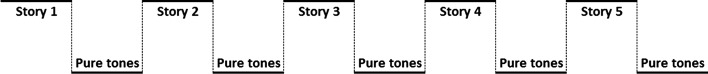
The block design of the fMRI experiment for story comprehension.
One hundred ten fMRI scans were obtained per subject during the narrative comprehension paradigm using a Bruker 3T Medspec (Bruker Medizintechnik, Karlsruhe, Germany) imaging system. The total scan time was 5 min and 30 sec, and the first 10 scans were discarded in order to allow the spins to reach relaxation equilibrium. Details of the EPI-fMRI parameters were TR/TE=3000/38 ms, BW=125 kHz, FOV=25.6 cm×25.6 cm, matrix=64×64, and slice thickness=5 mm. T1-weighted inversion recovery MDEFT scans were obtained from each subject for anatomical co-registration.
The fMRI data were preprocessed using in-house software written in Interactive Data Language (IDL; ITT Visual Information Solutions, Boulder, CO). A multi-echo reference scan (Schmithorst et al., 2006) was used for the correction of Nyquist ghosts and geometric distortion from B0 field inhomogeneity in image reconstruction (Schmithorst et al., 2001), and a pyramid iterative co-registration algorithm was used for motion correction (Thevenaz et al., 1998). The data were subsequently transformed into the stereotaxic space using linear affine transformation (Talairach and Tournoux, 1988).
The spectral graphical model with model averaging
The network construction consists of two main steps. In the first step, the group ICA is conducted to identify spatial-independent components of active brain regions. Once we identify these regions, each of them is regarded as a node in the network and then the spectral graphical model is applied to construct a connectivity network among these regions.
Group ICA
The preprocessed fMRI data were concatenated subject-wise and then a group spatial ICA was applied to identify activated brain regions involved in story comprehension (Calhoun et al., 2001; McKeown et al., 1998; Schmithorst and Holland, 2004). First Principal Component Analysis (PCA) was applied to reduce the data dimension in the time domain for each child. Then, the data were concatenated across subjects and the PCA was further applied on this grouped data set to reduce the temporal data dimension to 40. The Fast ICA algorithm (Hyvarinen, 1999) was repeated for 25 times, and a hierarchical agglomerative clustering algorithm (Himberg et al., 2004) was used to group IC components. Details of the group ICA method can be found in Schmithorst et al. (2006). In those IC clusters identified to be task related, active cortical regions are determined by a voxelwise one-sample t-test performed on the individual IC maps, with Bonferroni correction for multiple voxel comparisons. The task-related regions are also identified by a standard random effect GLM analysis (Karunanayaka et al., 2007). For each active brain region, the average of the fMRI signals from the maximum activation voxel and its six neighbors is chosen as the representative time series.
Neural network modeling with BN
BN have been extensively studied in Machine Learning and Statistics literature (Friedman and Goldszmidt, 1998; Geiger and Heckerman, 1994; Heckerman et al., 1995; Jordan, 1998) as a flexible structure learning technique. A BN is a directed acyclic graph (DAG) that encodes the causal relationships among a set of random variables. When applied to brain connectivity modeling, each node in the graph stands for a task-related brain region. Consider a BN of brain regions indexed by  , and let
  be the input data for the (k)th region. Under the model assumptions of DAG, the joint likelihood of the data given a DAG can be decomposed into a product of a series of conditional probabilities (Jordan, 1998) (Fig. 2):
FIG. 2.

The decomposition of the joint likelihood of data in Bayesian Networks (BN). Each likelihood is simplified into a product of local conditional probabilities based on the network structure (Jordan, 1998). Color images available online at www.liebertonline.com/brain
 |
(1) |
where πk denotes the multivariate time series for the parent regions of the (k)th region, S denotes the network of interest, and θS denotes the parameters in S. In recent BN applications to neural network construction (Zheng and Rajapakse, 2006), the inputs (Xk,t, πk,t) are assumed to be independent and discretized; thus, each conditional probability in Equation (1) can be written as  To select the most likely network from the list of possible ones, the Akaike information criterion (AIC) of the following form is commonly used (Akaike, 1974)
 |
(2) |
Here  is the maximum likelihood estimate of θS and qS denotes the effective number of parameters in the model.
Spectral density matrix of the network
In this section, we describe the graphical model approach (Bach and Jordan, 2004) for learning brain connectivity structure. In the remaining of the article, we will use the term “Spectral Bayesian Network” (SBN) for this graphical approach since it learns the network structure based on the spectral density matrix of the multivariate time-series input in the frequency domain. Let  be the M×T multivariate time series for M task-related active brain regions, where each row
  is the univariate time course representing the (k)th region. Denote
  as the (t)th column of X. Assuming that X is centered and stationary, the autocovariance function of X is an M×M matrix defined as
 |
(3) |
for any lag  . The off-diagonal elements in the sub block
  denote the cross-covariances of brain region k and its parent nodes πk. For a given h, this block describes the pairwise linear dependency between the brain regions in {k, πk}. The spectral density matrix of X is defined as
 |
(4) |
for  . The f(ω) is an M×M symmetric matrix with a fixed frequency ω, and the (i, j) entries from all the spectral matrices aggregate together to form a spectral decomposition of the temporal dependence between the activations in brain region i and j (Salvador et al., 2005, 2007) (Fig. 3). After applying Bayes' rule to the conditional probabilities in Equation (1), the AIC score of a given network S can be rewritten as
 |
(5) |
FIG. 3.

The estimated cross spectral density between two time series with different levels of connectivity strength, with 90% sample quartile intervals (dash line) in 1000 simulations. The bivariate time series are generated from VAR models as described in section Simulation studies, with connection parameter p=0.1 (top), 0.6 (middle), and 0.9 (bottom) for the link between the two time series. The sample mean and standard deviation of the differences of SBN AIC scores between the true network (connected) and the empty networks in the simulations are shown above the plots. AIC, Akaike information criterion; SBN, Spectral Bayesian Network; VAR, vector autoregressive. Color images available online at www.liebertonline.com/brain
This is a sum of likelihood  with respect to the network structure S, plus the penalty qS on network complexity. Assuming that the multivariate time-series
  are generated from a stationary Gaussian process, each local likelihood in Equation (5) can be approximated using the corresponding sub block in the spectral density matrix of X. plus a constant term C that does not depend on the network structure (Bach and Jordan, 2004; Jordan, 1998)
 |
(6) |
where  is an arbitrary set of the nodes in the graph, fA(ω) is the square block of f(ω) with respect to the nodes in A, and
  corresponds to the estimated spectral density of the input time-series X. The Appendix gives the complete derivation of the log likelihood estimate. The AIC score for the complete network can be written as
 |
(7) |
 |
(8) |
Here  is the maximum likelihood estimate of the spectral densities, and each
  in Equation (7) is a sub block of
  . In practice f(ω) is estimated by smoothing the periodograms of the multivariate time-series X at discrete frequencies ωj, resulting in a numerical integration in Equation (8). Gaussian spectral window is applied for periodogram smoothing (Appendix). Since the estimated spectral densities represent the cross-covariance of the brain activity among different regions in the frequency domain (Fig. 3), Equation (8) provides a concise selection criterion based on the dependency information across the whole spectrum, rather than depending on specific time lags.
Structure learning by Bayesian model averaging
The selection of the best network structure is a crucial step in the model. Many factors influence this decision process, and special care should be exercised to address this issue. The first concern is due to the high noise level of fMRI data. With such a noisy dataset, the best model chosen by the model selection criterion (for instance, using the AIC scores) is the best model for the contaminated data; thus, simply choosing the model with the smallest AIC score may lead to false identification of the true model. The second disadvantage of the traditional model selection procedures, such as AIC and Bayesian Information Criterion, lies in the fact that no prior network structure information can be incorporated into the selection. In brain imaging, researchers have garnered well-established neuro-anatomical knowledge over the years. It is unreasonable from a modeling perspective to ignore validated information about the brain during our network search procedures. The last issue is the notion of model equivalence in the learning of BN structure. In BN, two graphs are said to be equivalent if the factorization in Equation (1) based on one graph is identical to the factorization based on the other. When the estimation of network structure is the main focus, we need to distinguish the networks that are different yet have the same AIC score.
Observing these three issues, we propose the following Bayesian model averaging (BMA) approach to identify the optimal network structure. Instead of a direct comparison of all the competing networks, our method computes and ranks the posterior probability of the existence of a particular link given the observed data, and constructs the connectivity network by adding the most plausible link one at a time. Since these posterior probabilities are unique, the network identified using this procedure is also unique.
In BMA (Hoeting et al., 1999), the posterior distribution of an arbitrary variable of interest, Δ, given data D, can be written in the following form
 |
(9) |
where the posterior distribution p(Δ|D) is constructed by averaging K candidate models Mk. In learning network structures, each model Mk represents a candidate network Sk. The quantity of interest Δ is the existence of an edge  between two brain regions a and b. We further assume
  if the kth network structure Sk contains the edge
  , and
, and  if this edge is not in Sk. Our BMA approach for network construction is described by the following algorithm:
1. Choose
 as the pool of candidate network structures.
2. Compute the network score for each Sk in
 using the AIC metric in Equation (8).
-
3. Compute
 for each edge
  , from averaging over all networks in
  .
.
(10) An estimate of p(Sk|D) can be obtained when we compute AIC (Bozdogan, 1987).
-
4. Build the network.
a) Start with an empty graph S.
b) Consider all edges not in S, add the one with highest
 into S.
c) If cycle is formed, delete the current edge.
- d) Repeat b) and c) until no edges outside S satisfies
(11)
5. Output S.
The algorithm starts with an empty network and adds edges one by one into the graph according to their posterior probability averaging from the pool unless the current addition results in a cyclic graph, which is not allowed by the definition of BN. We build a network only with the connections supported by the data since all the edges with relative low posterior probability are excluded in the construction, which is controlled by the threshold C in Equation (11) (Jeffreys, 1998; Madigan and Raftery, 1994). Jeffreys (1998) and Madigan and Raftery (1994) suggest the use of a value between 0.1 and 0.001 analogous to p-values to exclude edge with significantly small posterior probability. In this article, we use  =0.05, which is a common choice of significance level in hypothesis testing. We have examined the impact of threshold
  in learning language network structure in the section Study on children's narrative comprehension, and the resulting networks are the same for C ranging from 0.01 to 0.1.
For the selection of  , we discard networks with relatively small posterior probabilities such that p(S|D)/max p(S|D)<C. This is because networks with very low posterior probabilities are generally very different from the ground truth. Discarding these poor candidate models will enable the model selection procedure to avoid substantial contribution to the sum in Equation (10) by a large number of unreasonable networks each contributing a small posterior probability. This is a common practice in BMA (Hoeting et al., 1999; Raftery et al., 1997). Again, we choose C=0.05. Furthemore, the computation in Equation (10) requires the estimation of the posterior probability for each candidate model. When the number of nodes in the network is moderate (which is the case for our narrative comprehension study), exhaustive computation over all the competing models is feasible. Since the number of the candidate models grows exponentially as the number of nodes increases, stochastic approximation may be needed for larger networks.
Results
Simulation studies
In this section we perform several simulations to demonstrate the robustness of the SBN model in detecting the network structure underlying multivariate time series. The results of the spectral model are compared with those of static BN and DBN. The multivariate time-series  are generated from a first-order VAR model. We consider a network with four nodes (M=4):
 |
(12) |
 |
where  is a four-dimensional observation at time t, and Φ is the 4×4 one-step connectivity matrix. Any nonzero off-diagonal entry Φij represents an unidirectional interaction from node Xi to node Xj. There is no connection in the graph for nodes Xi and Xj when Φi,j=Φj,i=0. The
  are assumed to be independent and identically distributed Gaussian noise with zero mean and diagonal covariance matrix σ2I4. To ensure that the time series are Gaussian and stationary, We assume X0 to be Gaussian with zero mean and diagonal covariance matrix
  . In this study, we examine three different connectivity matrices Φ with different levels of connections:
 |
(13) |
The corresponding network structures are demonstrated in Figure 4.
FIG. 4.

The three graphical structures for simulating four-dimensional multivariate time series from VAR models.
We consider a variety of parameter settings to test the robustness of SBN modeling. First, we study the effect of the length of observed time-series T when other parameters are fixed  Synthetic time series are generated with length ranging from 50 to 500 and the simulations are repeated 100 times. In each run we compute the graphs learned from each method and record the percentage of successful identification of the true network structure from which the time series are generated.
Figure 5 demonstrates the difference in terms of structural learning between ordinary BN (Zheng and Rajapakse, 2006), DBN (Rajapakse and Zhou, 2007), and our approach. The MATLAB software package, Bayes Net Toolbox (Murphy, 2001), is used for BN and DBN models. Clearly, SBN outperforms BN and DBN consistently in model identification, especially when the length of the time-series T is limited. When the true data generated network structure is complex (Φ1) a moderate T is necessary to guarantee the performance of SBN. For simpler structure as in Φ2 and Φ3 SBN can identify close to 100% of the true network when T ≥ 100, while both BN and DBN give poor results. Compared with DBN and SBN, the performance of BN is much worse. This is because the synthetic data are simulated with strong temporal correlation (autoregressive) especially in Φ1 and Φ2.
FIG. 5.

Percentage of identifying true structure under different signal lengths (T). Green: SBN. Blue: Dynamic Bayesian Networks (DBN). Red: Gaussian Bayesian Network without assuming temporal dependency. Time series are simulated from the three different graphs (Φ1, Φ2, Φ3) as shown in Figure 4.
Furthermore, we examine the impact of the connectivity strength on model performance when the observed time series have a moderate length (T=500) and a short length (T=100). Other parameters are fixed  Figure 6 shows that SBN can detect the right network structure under moderate connectivity strength (0.4≤p1≤0.9) when the observed time courses are of moderate length (T=500). Figure 7 shows that when the length of observation is limited (T=100), SBN can still learn the true network structure if the network has moderate numbers of connections (Φ2, Φ3) with relatively strong connectivity strengths. In both simulations, SBN models perform much better than BN and DBN unless the connectivity strength is weak (p1≤0.3). It is worth mentioning that the SBN approach is for learning the network structure instead of estimating the strength of any specific link in the network. Thus, although we validate the performance of SBN mainly using data from first-order VAR models, SBN can be applied to VAR models with longer lags or time series with other type of temporal structure.
FIG. 6.

Percentage of identifying true structure under different strengths of connectivity (p1) when the length of time-series T=500. Blue: SBN. Red: DBN. Green: Gaussian Bayesian Network without assuming temporal dependency. Time series are simulated from the three different graphs (Φ1, Φ2, Φ3) as shown in Figure 4.
FIG. 7.

Percentage of identifying true structure under different strengths of connectivity (p1) when the length of time-series T=100. Blue: SBN. Red: DBN. Green: Gaussian Bayesian Network without assuming temporal dependency. Time series are simulated from the three different graphs (Φ1, Φ2, Φ3 as shown in Figure 4.
Study on children's narrative comprehension
Six task-related spatial-independent components are identified using the procedure outlined in the section The spectral graphical model with model averaging in the narrative comprehension task (Schmithorst et al., 2006). The ICA maps displayed in Figure 8 show the activations in each task-related component. The components are ordered according to the phase of the averaged Fourier component relative to the reference on–off time course. The activated brain regions and activation foci are shown in Table 1. These task-related regions are also identified by a random-effect GLM analysis (Karunanayaka et al., 2007).
FIG. 8.

The six task-related networks (a-f) found from spatial group-independent component analysis of 313 children performing a narrative story comprehension task. The brain regions included in regions of interests (in the left and the right hemispheres) of each map are shown in Table 1. Slice range: Z=−25 to +50 mm (Talairach coordinates). All images are in radiological orientation. Extracted from Schmithorst et al. (2006).
Table 1.
Activation Foci (Talairach Coordinates) for the Task-Related Independent Component Analysis Components
| ICA component | Brain function | Brain region | BA | Coordinates (X,Y,Z) |
|---|---|---|---|---|
| a | Primary auditory cortex | L. superior temporal gyrus | 41 | −38, −21, 15 |
| R. superior temporal gyrus | 41 | 46, −21, 20 | ||
| b | Processing of auditory spectral and temporal information | L. superior temporal gyrus | 22 | −54, −13, 5 |
| R. superior temporal gyrus | 22 | 50, −17, 5 | ||
| c | Broca's Area and left lateralized phonological working memory network | L. medial temporal gyrus | 21 | −54, −33, 0 |
| L. inferior frontal gyrus | 46 | −38, 43, 5 | ||
| L. inferior frontal gyrus | 44/45 | −42, 7, 30 | ||
| L. inferior parietal lobule | 40 | −50, −53, 30 | ||
| L. middle frontal gyrus | 8 | −6, 23, 45 | ||
| d | Memory encoding and storage of narrative elements | L. hippocampus | −26, −25, −5 | |
| R. hippocampus | 22, −21, −5 | |||
| e | Wernicke's Area. Acoustic word recognition | L. superior temporal gyrus | 22 | −50, −49, 15 |
| R. superior temporal gyrus | 22 | 46, −53, 10 | ||
| f | Higher order semantic processing | L. angular gyrus | 39 | −46, −53, 25 |
| R. angular gyrus | 39 | 46, −49, 25 | ||
| L. precuneus/posterior cingulate | 7/31 | −10, −45, 30 |
Talairach coordinates were extracted from Schmithorst et al. (2006).
ICA, independent component analysis; BA, Brodmann area; L., left; R., right.
Two knowledge-based anatomical networks of language comprehension circuit have been proposed (Fig. 9) (Karunanayaka et al., 2007). The extended language network includes six regions of interest (ROI) that are identified by ICA: Brodmann area (BA) 22, BA 22 posterior, BA 39, BA 41, BA 44, and hippocampus. A simplified structure was also suggested in Karunanayaka et al. (2007), which does not include hippocampus (Fig. 8d). The simplified structure is more consistent with the Wernicke-Geschwind model and previous neuro-anatomical results, and is the focus in the study using linear SEM (Karunanayaka et al., 2007). Thus, in this article, we apply the SBN approach with model averaging to learn the network connectivity among the five brain regions represented by the independent components a, b, c, e, and f, which encompass Brodmann Areas BA 22, BA 22 posterior, BA 39, BA 41, and BA 44. We compare our results with the simplified network (Figure 9) proposed based on neuro-anatomical knowledge.
FIG. 9.

Knowledge-based neural/brain network for narrative story comprehension. The simplified network does not include the hippocampus identified in IC d. The Talairach coordinates of the activation foci are shown in Table 1.
For each of the five ROIs, a representative fMRI time series is selected by averaging from the voxel of maximum activation and all its neighboring voxel per hemisphere per children. We divide the subjects into three age groups: 5 to 8, 9 to 13, and 14 to 18 years old. For each age group, the structures of the neural functional networks in both left and right hemisphere are estimated using SBN with model averaging. The input to SBN for each age group is the median time series from all subjects within the age range. For the left hemisphere, we consider a five-node network among BA 22, BA 22 posterior, BA 39, BA 41, and BA 44, and for the right hemisphere, we only look at the network of BA 22, BA 22 posterior, BA 39, and BA 41. We omitted BA 44 (Broca's area) from the right hemisphere model because this region did not reach significance in the first-level analysis with ICA or GLM and is not considered to be functionally related to narrative comprehension.
Our model selection procedure searches among all the models in the candidate pool S and decides the most probable set of links. Thus, the choice of pool S is very important. First, we restrict S to only contain networks starting from brain region BA 41, which is a well-accepted anatomical result since BA 41 corresponds to the primary auditory cortex for the initial processing of acoustic information. Furthermore, instead of averaging from all possible neural networks with no edge pointed to BA 41, we discard networks with relative small posterior probability such that p(S | D)/max p(S | D)<0.05. Using the edge score in Equation (10), we computed the posterior probability of the existence of all possible connections among the task-related regions and then the network structure is constructed using the averaging algorithm outlined in the section Structure learning by Bayesian model averaging.
Figure 10 shows the connectivity network learned for the left hemisphere. The estimated networks stand for the average neural connectivity predicted during the task of narrative comprehension in children ranging in age from 5 to 8, 9 to 13, and 14 to 18 years. Most of the estimated pathways predicted are highly consistent among the three age groups except the links from BA 41 to BA 39 in the 5–8 group and from BA 41 to BA 44 in the 14–18 group. The edge scores computed based on model averaging are shown in Table 2. All the edge scores have been rescaled for each age group separately such that Σk p(Sk | D)=1.The connections from BA 41 to BA 22 and from BA 22 to BA 44 show the highest edge scores across three groups, which suggest a pathway with relative high connectivity magnitude through these regions in all these development stage of children. Of particular importance, we observe that the youngest age group of children have a strong connection (edge score 0.440) between primary auditory cortex (BA 41) and auditory-language association areas (BA 39) that is not detected in the older age groups of children. Instead, the oldest children exhibit a long-range connection (edge score 0.841) between primary auditory cortex (BA 41) and Broca's area (BA 44) along the arcuate fasiculus. The weak connection between BA22 and BA39 in the left hemisphere (connection strength<0.2 for all age groups in Table 2) is consistent with our understanding of the language network connections within the brain in that the anterior part of BA22 is directly involved with phonological processing while the posterior part of BA22 (BA22 posterior) is traditionally referred to as Wernicke's Area for language processing and feeds forward into language association areas in the Angular gyrus (BA39) (Catani and Jones, 2004; Karunanayaka et al., 2007).
FIG. 10.

The estimated neural network for narrative story comprehension in the left hemisphere for three different age groups—5 to 8 (top), 9 to 13 (middle), and 14 to 18 (bottom)—based on the Bayesian averaged network that utilized a network scoring criterion as part of the SBN approach. Green edges are the connections not identified in all the age groups.
Table 2.
Edge Scores in the Functional Networks Learned for Both Hemispheres in Each Age Group
| Start region | End region | Age 5–8 | Age 9–13 | Age 14–18 |
|---|---|---|---|---|
| Left hemisphere | ||||
| BA 22 (IC b) | BA 22 Post (IC e) | 0.535 | 0.818 | 0.555 |
| BA 22 (IC b) | BA 39 (IC f) | 0.180 | 0.195 | 0.084 |
| BA 22 (IC b) | BA 44 (IC c) | 0.937 | 0.864 | 0.955 |
| BA 22 Post (IC e) | BA 39 (IC f) | 0.584 | 0.766 | 0.955 |
| BA 22 Post (IC e) | BA 44 (IC c) | 0.937 | 0.864 | 0.538 |
| BA 41 (IC a) | BA 22 (IC b) | 0.937 | 0.864 | 0.955 |
| BA 41 (IC a) | BA 22 Post (IC e) | 0.567 | 0.092 | 0.800 |
| BA 41 (IC a) | BA 39 (IC f) | 0.440 | ||
| BA 41 (IC a) | BA 44 (IC c) | 0.841 | ||
| Right hemisphere | ||||
| BA 22 (IC b) | BA 22 Post (IC e) | 0.853 | 0.976 | 0.760 |
| BA 22 Post (IC e) | BA 39 (IC f) | 0.802 | 0.976 | 0.958 |
| BA 41 (IC a) | BA 22 (IC b) | 0.924 | 0.976 | 0.958 |
| BA 41 (IC a) | BA 22 Post (IC e) | 0.396 | ||
The edge score of an effective connection between two brain regions is computed using the Bayesian averaging approach defined in equation (10). The edge scores have been rescaled in each group so that the sum of the posterior probabilities of the candidate networks is one.
With no activation identified in BA 44 in the right hemisphere, Figure 11 shows the estimated networks among BA 22, BA 22 posterior, BA 39, and BA 41 for children in three different age groups in the right hemisphere. Similar to the networks learned for the left hemisphere, the network structures are highly consistent among the groups. The eldest age group shows an additional path from BA 41 to BA 22 Posterior, which is not present in the two younger age groups, but its score is relatively low compared with all other edges in the network. A single pathway, BA41→BA 22→BA 22 posterior→BA 39 is learned by the model averaging algorithm, which is a simpler connectivity structure compared with its counterpart in the left hemisphere.
FIG. 11.

The estimated neural network for narrative story comprehension in the right hemisphere for three different age groups—5 to 8 (top), 9 to 13 (middle), and 14 to 18 (bottom)—based on the Bayesian averaged network that utilized a network scoring criterion as part of the SBN approach. Green edges are the connections not identified in all the age groups.
Discussion & Future Work
In this article, we applied the spectral graphical model with model averaging to construct brain connectivity networks using fMRI data. The advantage of our approach is three-fold. First, it assumes only a standard a priori constraint on the network structure and the algorithm can select the most probable network based on data. Second, this approach utilizes the fMRI signals transformed into the frequency domain to build a spectral graphical model; thus, the temporal characteristic of the entire time series are accounted for. This is fundamentally different from the BN and DBN approaches (Rajapakse and Zhou, 2007; Zheng and Rajapakse, 2006), where the data are assumed to follow an autoregressive process with fixed lags (DBN) or no lag (BN). Third, we adopt the BMA technique for model selection, which is less sensitive to noise and more robust against outliers.
Previous network models (Karunanayaka et al., 2007) proposed for this narrative comprehension task have used a linear deterministic modeling approach (structural equation model) that requires a rigidly defined set of a priori network elements and links between them. The current treatment using SBN with model averaging is more flexible than the SEM approach because it does not require a priori definition of all the network elements and connections. Instead, the optimization of the network in the frequency domain can generate new graphs that include connections that were not predicted a priori. Moreover, compared with other BN (BN, DBN) that have been applied to the structure learning of neural networks using fMRI data, the SBN approach considers the whole spectrum (and thus the whole autocovariance function, Γ(h), h ≥ 0) of the fMRI time series in the approximation of the likelihood function, while the applications using other BN only considered fixed lags such as Γ(1) and Γ(0) (Li et al., 2008; Rajapakse and Zhou, 2007; Zheng and Rajapakse, 2006).
The Dynamic Causal Models (DCM) are another popular class of network models that do not rely on the autoregressive assumptions of the underlying time series (Friston et al., 2003, 2011; Penny et al., 2004a, 2004b). Instead, DCM captures the network structure by tuning model parameters that minimize the difference between the predicted output of a dynamic system and the observed time series. In comparison, our approach is fundamentally different from DCM in two respects. DCM is built upon time domain data, whereas our model is based on the spectral domain and has the flexibility of examining network structure of different frequency bands. DCM utilizes the Bayesian model selection criterion to choose the optimal network, whereas our method adopts the BMA concept for stepwise selection of the best connections. In this article, we focus on demonstrating the applicability of the SBN for learning brain connectivity network. A detailed comparative study between DCM and SBN is currently under investigation.
In our treatment of the connectivity in the narrative comprehension network, the left and right hemispheres are modeled separately. This approach was used for two reasons. First, the activation patterns corresponding to this task have been found for the right and left hemispheres in both children and adults using conventional GLM analysis (Holland et al., 2007; Schmithorst et al., 2006) as well as ICA (Karunanayaka et al., 2007). Further, the literature on hemispheric dominance has demonstrated that left and right hemisphere networks for language processing are asymmetric by multiple imaging and behavioral methods, including fMRI, PET, Transcranial Doppler ultrasound, Dichotic listening tests, and lesion studies (Lohmann et al., 2005; Petersen et al., 2000; Springer et al., 1999). Between 92% and 96% of right-handed adults are left dominant for language processing in the brain (Springer et al., 1999) and diffusion MRI tractography has gone so far as to demonstrate that the arcuate fasciculus, the major white matter pathway connecting key language regions in the left hemisphere, is incomplete in left-dominant individuals (Catani et al., 2007). Clearly, cooperation between hemispheres is important for this task and the presented data demonstrate a high degree of symmetry in the pattern of activation. Therefore, it is appropriate to consider the interaction between the hemispheres for this task. However, considering a bi-hemisphere network, the number of nodes becomes 10 to 14, requiring a much longer observed time series to guarantee the model performance. The simulations included in Figures 5–7 demonstrate that our algorithm needs a longer time series to accurately estimate connection strengths in larger networks. Thus, we decide to investigate the intra-hemisphere networks only, given the limitations of the fMRI data we have from this group of children.
The left hemisphere SBN model differs somewhat from the knowledge-based model in that the expected feed forward connection between IC f (BA 39 located in the Angular Gyrus) to IC c, which includes BA 44 (Broca's Area) in the inferior frontal gyrus, was not predicted. Instead, the Bayesian model predicts connections to Broca's Area arising directly from Wernicke's area IC e (BA 22 posterior) and IC b (BA 22). The SBN approach also detected two age-dependent connections in the left-hemisphere language network for the narrative comprehension task. These can be seen in Figure 10 and in Table 2. An additional connection leading directly from IC a in the superior temporal gyrus (BA 41 auditory cortex) to IC c (BA 44), shown in Figure 10c as a dashed line, was predicted in the 14–18-year-old age group but not in the two younger groups of children. Such a connection is plausible given the strong connections between auditory and language areas along the path of the arcuate fasciculus in the brain. In the 5–8-year-old group, SBN predicts a connection directly from IC a (BA 41) to IC f (BA 39), which vanishes in the older age groups. These data-driven predictions can provide a basis for revision and refinement of language network models and the influence of brain development on them.
The weak edge scores predicted for all age groups between the anterior portion of BA 22 in the superior temporal gyrus and BA 39 in the Angular gyrus in the left hemisphere are expected based on earlier findings (Karunanayaka et al., 2007). Recent findings from diffusion tractography imaging elegantly demonstrate the physical pathways associated with the left-dominant language network along the acruate fasiculus as including the connection from BA22 posterior to BA39 (Catani and Jones, 2004; Catani et al., 2007). So, the SBN predictions of strong connectivity along this pathway are satisfying in that they are in line with anatomical findings as well as connectivity estimates based on other techniques.
The SBN models for the right hemisphere focus on the 4-node network among the auditory and posterior language areas (ICs a, b, e, and f) for the narrative comprehension task as diagramed in Figure 11. This prediction is consistent with recent neuro-anatomical findings based on diffusion tensor imaging that demonstrate strong asymmetry between left- and right-hemisphere white matter connections along the arcuate fasciculus pathway (Catani and Jones, 2004; Catani et al., 2007). Right-hemisphere networks selected by SBN were identical for the two younger age groups of children but included an additional connection between auditory cortex (BA 41) and Wernicke's area (BA 22 posterior) in the oldest group of 14–18-year-olds (Table 2). This may correspond with continued myelination in late adolescence (Toga et al., 2006).
The application of the network learning approach proposed here using SBN to model language connectivity network in the developing brain provides a gnomic demonstration of the flexibility of this method to predict changing connectivity in networks as a function of physiological or behavioral variables. In this case the age grouping of the subjects is used to demonstrate that different connections are important during development. A similar approach could be used in the future to examine data from patients with neurological diseases such as epilepsy, stroke, or aphasia. In that case, connectivity strength predicted by the graphs could pinpoint deficits in network connections that underlie symptoms of the disorder. The simulations show us that the SBN approach can correctly predict the networks structure, provided a sufficient sample of the temporal network behavior is available. The results in children of different ages shown in Figures 10 and 11 go one step further and demonstrate the power of this graphical modeling approach for predicting the dynamic evolution of network connectivity—in this case as a function of subject age.
As a nonparametric approach to approximate the model selection criterion (AIC) using frequency-domain data instead of building specific parametric model in the time domain, the SBN model prefers a longer time series for better performance in network structure learning as shown in the simulations. Typical fMRI experiments contain 100–250 time-series samples. For conventional fMRI statistical analysis, this time series is available for each voxel in each slice of the brain image volume. Future work using the SBN approach to estimate task-related brain connectivity could benefit from data sets with higher sampling rate and longer time-series. fMRI has limitations on the sampling rate that limit it to a second or more, depending on the number of slices acquired at each time point. However, other brain imaging techniques such as EEG or MEG can provide time-series data with much higher sampling rates of 5 kHz or greater. Group ICA of fMRI data to generate the network model combined with SBN of MEG data from the same task might permit better estimates of connection strengths and variability with age, handedness, or gender in a whole-brain bi-hemisphere functional network in the future.
Appendix
In a Spectral Bayesian Network (SBN) model of M×T multivariate time-series  , where M is the number of nodes (brain regions) in the network and T is the length of time series, the likelihood is first decomposed based on the network structure S as in static Bayesian Networks (BN):
 |
where Xk and πk denotes the (multivariate) time series of the (k)th nodes and the parent nodes of the (k)th nodes, respectively, and θS denotes the collection of parameters in all the local probability distributions above. The distributions p(Y|S,θS), Y={Xk, πk} or  cannot be further decomposed as in Equation (2) since Y is indeed a subset of the multivariate time-series X. Instead, when T is long enough, each local log-likelihood logp(Y|S,θS) can be estimated by
 |
where h (Y) is the entropy rate of the time series given that it is a finite sample of a stationary ergodic process. This approximation is based on the asymptotic equipartition property:  . This is also known as the Shannon-McMillian-Breiman theorem in information theory (Cover et al., 1991). Assuming the stationary and Gaussianity for the multivariate time-series Y, the entropy rate can be computed from spectral densities directly
 |
where e is the natural number, MY is the dimension of Y, and fy(ω) is the MY×MY spectral density matrix of Y. Thus, the Akaike information criterion (AIC) score for a Spectral BN can be aggregated as
 |
where  are the spectral density estimates corresponding to the set of nodes Y, and C=M log 2πe/2 is a constant independent of the network structure. Suppose we have a set of discrete estimation of f(ω) at Fourier frequencies, the integration above can be further approximated by interpolations and the AIC score in SBN modeling is
 |
where the constant term is ignored. The Gaussian spectral window  is applied to smooth the peridograms to obtain the spectral density estimate. The optimal smoothing parameter σ is chosen by applying the AIC on the whittle approximation of the likelihood of the multivariate time series. We follow Bach and Jordan (2004) to use
  as the penalty of the network complexity where T* is the effective length of the spectral density sequence after smoothing.
Acknowledgment
This work was funded in part by a grant from the NIH: R01-HD38578.
Author Disclosure Statement
No competing financial interests exist.
References
- Akaike H. A new look at the statistical model identification. IEEE Trans Autom Control. 1974;19:716–723. [Google Scholar]
- Bach F. Jordan M. Learning graphical models for stationary time series. IEEE Trans Signal Process. 2004;52:2189–2199. [Google Scholar]
- Barthes R. Duisit L. An introduction to the structural analysis of narrative. New Literary Hist. 1975;6:237–272. [Google Scholar]
- Bozdogan H. Model selection and Akaike's information criterion (AIC): the general theory and its analytical extensions. Psychometrika. 1987;52:345–370. [Google Scholar]
- Buchel C. Friston K. Modulation of connectivity in visual pathways by attention: cortical interactions evaluated with structural equation modelling and fMRI. Cereb Cortex. 1997;7:768. doi: 10.1093/cercor/7.8.768. [DOI] [PubMed] [Google Scholar]
- Bullmore E. Horwitz B. Honey G. Brammer M. Williams S. Sharma T. How good is good enough in path analysis of fMRI data? Neuroimage. 2000;11:289–301. doi: 10.1006/nimg.2000.0544. [DOI] [PubMed] [Google Scholar]
- Burge J. Lane T. Link H. Qiu S. Clark VP. Discrete dynamic Bayesian network analysis of fMRI data. Hum Brain Mapp. 2009;30:122–137. doi: 10.1002/hbm.20490. [DOI] [PMC free article] [PubMed] [Google Scholar]
- Calhoun V. Adali T. Pearlson G. Pekar J. A method for making group inferences from functional MRI data using independent component analysis. Hum Brain Mapp. 2001;14:140–151. doi: 10.1002/hbm.1048. [DOI] [PMC free article] [PubMed] [Google Scholar]
- Catani M. Allin M. Husain M. Pugliese L. Mesulam M. Murray R. Jones D. Symmetries in human brain language pathways correlate with verbal recall. Proc Natl Acad Sci U S A. 2007;104:17163. doi: 10.1073/pnas.0702116104. [DOI] [PMC free article] [PubMed] [Google Scholar]
- Catani M. Jones D. Perisylvian language networks of the human brain. Ann Neurol. 2004;57:8–16. doi: 10.1002/ana.20319. [DOI] [PubMed] [Google Scholar]
- Cover TM. Thomas JA. Wiley J. Elements of Information Theory. 1991. Wiley Online Library.
- Friedman N. Goldszmidt M. Learning Bayesian networks with local structure; Proceedings of the Twelfth Conference on Uncertainty in Artificial Intelligence; San Francisco, California, USA; 1996. pp. 252–262. [Google Scholar]
- Friston K. Causal modelling and brain connectivity in functional magnetic resonance imaging. PLoS Biol. 2009;7:e1000033. doi: 10.1371/journal.pbio.1000033. [DOI] [PMC free article] [PubMed] [Google Scholar]
- Friston K. Harrison L. Penny W. Dynamic causal modelling. Neuroimage. 2003;19:1273–1302. doi: 10.1016/s1053-8119(03)00202-7. [DOI] [PubMed] [Google Scholar]
- Friston KJ. Li B. Daunizeau J. Stephan KE. Network discovery with DCM. Neuroimage. 2011;56:1202–1221. doi: 10.1016/j.neuroimage.2010.12.039. [DOI] [PMC free article] [PubMed] [Google Scholar]
- Geiger D. Heckerman D. Learning Gaussian Networks; Proceedings of the Tenth Conference on Uncertainty in Artificial Intelligence; Seattle, Washington, USA; 1994. pp. 235–243. [Google Scholar]
- Heckerman D. Geiger D. Chickering D. Learning Bayesian networks: the combination of knowledge and statistical data. Mach Learn. 1995;20:197–243. [Google Scholar]
- Himberg J. Hyvarinen A. Esposito F. Validating the independent components of neuroimaging time series via clustering and visualization. Neuroimage. 2004;22:1214–1222. doi: 10.1016/j.neuroimage.2004.03.027. [DOI] [PubMed] [Google Scholar]
- Hoeting J. Madigan D. Raftery A. Volinsky C. Bayesian model averaging: a tutorial. Stat Sci. 1999;14:382–401. [Google Scholar]
- Holland SK. Vannest J. Mecoli M. Jacola LM. Tillema JM. Karunanayaka PR. Schmithorst VJ. Yuan W. Plante E. Byars AW. Functional MRI of language lateralization during development in children. Int J Audiol. 2007;46:533–551. doi: 10.1080/14992020701448994. [DOI] [PMC free article] [PubMed] [Google Scholar]
- Hyvarinen A. Fast and robust fixed-point algorithms for independent component analysis. IEEE Trans Neural Netw. 1999;10:626–634. doi: 10.1109/72.761722. [DOI] [PubMed] [Google Scholar]
- Jeffreys S. Theory of Probability. New York, NY: Oxford University Press; 1998. [Google Scholar]
- Jordan M. Learning in Graphical Models. Cambridge, MA: MIT Press; 1998. [Google Scholar]
- Karunanayaka P. Holland S. Schmithorst V. Solodkin A. Chen E. Szaflarski J. Plante E. Age-related connectivity changes in fMRI data from children listening to stories. Neuroimage. 2007;34:349–360. doi: 10.1016/j.neuroimage.2006.08.028. [DOI] [PubMed] [Google Scholar]
- Li J. Wang Z. Palmer S. McKeown M. Dynamic Bayesian network modeling of fMRI: a comparison of group-analysis methods. Neuroimage. 2008;41:398–407. doi: 10.1016/j.neuroimage.2008.01.068. [DOI] [PubMed] [Google Scholar]
- Lohmann H. Drager B. Muller-Ehrenberg S. Deppe M. Knecht S. Language lateralization in young children assessed by functional transcranial Doppler sonography. Neuroimage. 2005;24:780–790. doi: 10.1016/j.neuroimage.2004.08.053. [DOI] [PubMed] [Google Scholar]
- Lorch EP. Milich R. Sanchez RP. Story comprehension in children with ADHD. Clin Child Fam Psychol Rev. 1998;1:163–178. doi: 10.1023/a:1022602814828. [DOI] [PubMed] [Google Scholar]
- Madigan D. Raftery A. Model selection and accounting for model uncertainty in graphical models using Occam's window. J Am Stat Assoc. 1994;89:1535–1546. [Google Scholar]
- Mclntosh A. Gonzalez-Lima F. Structural equation modeling and its application to network analysis in functional brain imaging. Hum Brain Mapp. 1994;2:2–22. [Google Scholar]
- McIntosh A. Grady C. Ungerleider L. Haxby J. Rapoport S. Horwitz B. Network analysis of cortical visual pathways mapped with PET. J Neurosci. 1994;14:655. doi: 10.1523/JNEUROSCI.14-02-00655.1994. [DOI] [PMC free article] [PubMed] [Google Scholar]
- McKeown M. Makeig S. Brown G. Jung T. Kindermann S. Bell A. Sejnowski T. Analysis of fMRI data by blind separation into independent spatial components. Hum Brain Mapp. 1998;6:160–188. doi: 10.1002/(SICI)1097-0193(1998)6:3<160::AID-HBM5>3.0.CO;2-1. [DOI] [PMC free article] [PubMed] [Google Scholar]
- Murphy K. The bayes net toolbox for matlab. Comput Sci Stat. 2001;33:1024–1034. [Google Scholar]
- Penny W. Stephan K. Mechelli A. Friston K. Modelling functional integration: a comparison of structural equation and dynamic causal models. Neuroimage. 2004a;23:S264–S274. doi: 10.1016/j.neuroimage.2004.07.041. [DOI] [PubMed] [Google Scholar]
- Penny W. Stephan K. Mechelli A. Friston K. Comparing dynamic causal models. Neuroimage. 2004b;22:1157–1172. doi: 10.1016/j.neuroimage.2004.03.026. [DOI] [PubMed] [Google Scholar]
- Petersen S. Fox P. Posner M. Mintun M. Raichle M. Positron emission tomographic studies of the cortical anatomy of single-word processing. Nature. 1988;331:585–589. doi: 10.1038/331585a0. [DOI] [PubMed] [Google Scholar]
- Raftery A. Madigan D. Hoeting J. Model selection and accounting for model uncertainty in linear regression models. J Am Stat Assoc. 1997;92:179–191. [Google Scholar]
- Rajapakse J. Zhou J. Learning effective brain connectivity with dynamic Bayesian networks. Neuroimage. 2007;37:749–760. doi: 10.1016/j.neuroimage.2007.06.003. [DOI] [PubMed] [Google Scholar]
- Roebroeck A. Formisano E. Goebel R. Mapping directed influence over the brain using Granger causality and fMRI. Neuroimage. 2005;25:230–242. doi: 10.1016/j.neuroimage.2004.11.017. [DOI] [PubMed] [Google Scholar]
- Salvador R. Achard S. Bullmore E. Frequency-dependent functional connectivity analysis of fMRI data in Fourier and wavelet domains. In: Jirsa VK, editor; McIntosh AR, editor. Handbook of Brain Connectivity. New York, NY: Springer-Verlag; 2007. pp. 379–401. [Google Scholar]
- Salvador R. Suckling J. Schwarzbauer C. Bullmore E. Undirected graphs of frequency-dependent functional connectivity in whole brain networks. Philos Trans R Soc B: Biol Sci. 2005;360:937. doi: 10.1098/rstb.2005.1645. [DOI] [PMC free article] [PubMed] [Google Scholar]
- Schmithorst V. Dardzinski B. Holland S. Simultaneous correction of ghost and geometric distortion artifacts in EPI using a multi-echo reference scan. IEEE Trans Med Image. 2001;20:535. doi: 10.1109/42.929619. [DOI] [PMC free article] [PubMed] [Google Scholar]
- Schmithorst V. Holland S. A Comparison of three methods for generating group statistical inferences from independent component analysis of fMRI data. J Magn Reson Imaging. 2004;19:365. doi: 10.1002/jmri.20009. [DOI] [PMC free article] [PubMed] [Google Scholar]
- Schmithorst V. Holland S. Plante E. Cognitive modules utilized for narrative comprehension in children: a functional magnetic resonance imaging study. Neuroimage. 2006;29:254–266. doi: 10.1016/j.neuroimage.2005.07.020. [DOI] [PMC free article] [PubMed] [Google Scholar]
- Springer JA. Binder JR. Hammeke TA. Swanson SJ. Frost JA. Bellgowan PSF. Brewer CC. Perry HM. Morris GL. Mueller WM. Language dominance in neurologically normal and epilepsy subjects. Brain. 1999;122:2033. doi: 10.1093/brain/122.11.2033. [DOI] [PubMed] [Google Scholar]
- Talairach J. Tournoux P. Co-Planar Stereotaxic Atlas of the Human Brain. New York: Thieme; 1988. [Google Scholar]
- Thevenaz P. Ruttimann UE. Unser M. A pyramid approach to subpixel registration based on intensity. IEEE Trans Image Process. 1998;7:27–41. doi: 10.1109/83.650848. [DOI] [PubMed] [Google Scholar]
- Toga AW. Thompson PM. Sowell ER. Mapping brain maturation. Trends Neurosci. 2006;29:148–159. doi: 10.1016/j.tins.2006.01.007. [DOI] [PMC free article] [PubMed] [Google Scholar]
- Zheng X. Rajapakse JC. Learning functional structure from fMR images. Neuroimage. 2006;31:1601–1613. doi: 10.1016/j.neuroimage.2006.01.031. [DOI] [PubMed] [Google Scholar]