Chemical Shift Encoded Water–Fat Separation Using Parallel Imaging and Compressed Sensing

Abstract

Chemical shift encoded techniques have received considerable attention recently because they can reliably separate water and fat in the presence of off-resonance. The insensitivity to off-resonance requires that data be acquired at multiple echo times, which increases the scan time as compared to a single echo acquisition. The increased scan time often requires that a compromise be made between the spatial resolution, the volume coverage, and the tolerance to artifacts from subject motion. This work describes a combined parallel imaging and compressed sensing approach for accelerated water–fat separation. In addition, the use of multiscale cubic B-splines for B₀ field map estimation is introduced. The water and fat images and the B₀ field map are estimated via an alternating minimization. Coil sensitivity information is derived from a calculated k-space convolution kernel and l₁-regularization is imposed on the coil-combined water and fat image estimates. Uniform water–fat separation is demonstrated from retrospectively undersampled data in the liver, brachial plexus, ankle, and knee as well as from a prospectively undersampled acquisition of the knee at 8.6x acceleration.

Chemical shift-based water–fat separation methods are routinely used in the clinical MRI setting to separate unwanted species from the signal of interest to provide a clear visualization of pathology. These methods have been used for “fat-only” imaging to detect fatty infiltration in the myocardium (1) and to measure adipose tissue volume (2). Alternatively, these methods have been used for “water-only” imaging to visualize cartilage injury and meniscal tears in the knee (3) and to detect disease in the spine (4). Fat saturation techniques, such as chemical shift selective imaging (CHESS) (5), are a commonly used chemical shift-based method. Although versatile and widely applicable, fat saturation techniques are sensitive to B₀ inhomogeneity, which can result in incomplete suppression in regions of off-resonance (6). Chemical shift encoded techniques (7–10) have received considerable attention because they can reliably separate water and fat in the presence of off-resonance. These techniques acquire data at multiple (typically 2–3) echo times (TEs) and estimate the water and fat signals by correcting for the phase errors caused by B₀ inhomogeneity. Multiple works have demonstrated robust water–fat separation in the presence of high off-resonance (11–18).

The insensitivity to off-resonance of chemical shift encoded techniques requires that data be collected at multiple TEs, which increases the scan time as compared to a single echo acquisition. The increased scan time often requires that a compromise be made between the spatial resolution, the volume coverage, and the tolerance to motion artifacts. To address this compromise, scan time reduction techniques have been used. Both Hines et al. (19) and Yu et al. (20) have reported using parallel imaging (21,22) to shorten the scan time. Reeder et al. have developed a homodyne reconstruction technique for partial k-space acquisitions (23), whereas Brodsky et al. (24) and Bornert et al. (25) have proposed reconstruction methods for non-Cartesian acquisitions. Recent works from Doneva et al. (26) and Sharma et al. (27) have applied compressed sensing (28) by estimating the B₀ field map and the water and fat images directly from the undersampled k-space measurements.

In this work, we introduce a combined parallel imaging and compressed sensing approach for water–fat separation. The combination of these two techniques exploits complementary pieces of information; specifically, parallel imaging uses the distinct spatial sensitivities of the multiple receiver elements while compressed sensing makes use of the presumed compressibility of the desired images. We also introduce the use of multiscale cubic B-splines for estimating the B₀ field map. The water and fat images and the B₀ field map are estimated in an alternating manner directly from the undersampled k-space measurements. In the following section, we present the signal model and details of the reconstruction. Results using the proposed approach are then shown on liver, brachial plexus, ankle, and knee datasets, and these results are compared to those from an existing parallel imaging and water–fat separation technique. Finally, we discuss the benefits and limitations of the present work.

METHODS

Signal Model

We model, in Eq. 1, the undersampled k-space measurements from all receiver coils at all TEs, k_u, as a function of the unknown un-normalized coil sensitivities (C̃), unknown water and fat spin density images (ρ̃), unknown B₀ field map (represented in Ψ), known water–fat chemical shift modeling matrix (A), and known k-space sampling (F_u), in the presence of additive Gaussian noise with zero mean and unknown covariance matrix Σ.

$${\mathbf{k}}_{\mathbf{u}}={\mathbf{F}}_{\mathbf{u}}\stackrel{\sim }{\mathbf{C}}\mathbf{\Psi }\text{A}\stackrel{\sim }{\mathbf{\rho }}+\mathbf{N}(0,\mathbf{\sum })$$ [1]

The vector ρ̃ is a concatenation of the water spin density and the fat spin density images (i.e., $\stackrel{\sim }{\mathbf{\rho }}=[{\stackrel{\sim }{\rho }}_w^1;{\stackrel{\sim }{\rho }}_f^1;\dots {\stackrel{\sim }{\rho }}_w^P;{\stackrel{\sim }{\rho }}_f^P]$), where the subscript denotes the species and the superscript denotes the pixel index. The matrix A operates pixel-wise and we assume a six-peak fat spectrum with known relative amplitudes and frequency shifts (29). The block diagonal matrix Ψ contains exp(j2πψ^pt_n) on the pth diagonal of the nth block, where ψ^p is the field map value (in Hertz) at the pth pixel and t_n is the time (in seconds) of the nth echo.

In practice, the coil sensitivity maps are normalized such that the l₂-norm taken across the coil dimension is equal to one for all pixels. This is reflected by a slight modification of the signal model (Eq. 2), where C represents the normalized coil sensitivities and ρ denotes the coil-combined water and fat images, which are the water and fat spin density images multiplied by the square root sum of squares of the coil sensitivities.

$${\mathbf{k}}_{\mathbf{u}}={\mathbf{F}}_{\mathbf{u}}\mathbf{C}\mathbf{\Psi }\text{A}\mathbf{\rho }+\mathbf{N}(0,\mathbf{\sum })$$ [2]

Equation 2 presents the signal model that relates the unknowns (C, Ψ, ρ) to the measurements (k_u). Note that the product CΨAρ represents the echo time images from all coils. The undersampled Fourier transform, F_u, is applied to each image to yield the k-space measurements.

Sampling Considerations

The sampling of k-space should satisfy requirements for both parallel imaging and compressed sensing. From a k-space-based parallel imaging perspective, the sampling should avoid large regions of nonsampled points. This ensures that the k-space kernel can use acquired k-space points to synthesize the neighboring nonacquired points. The theory underlying compressed sensing suggests that the measurement vectors exhibit incoherence, where the coherence of a measurement matrix M is defined as the maximum off-diagonal absolute value of the matrix M^H·M (30). The measurement matrix in this work is F_uCΨAW⁻¹, where W represents the sparsifying transform. Because C will vary between scans and Ψ will vary both between scan and within one reconstruction, a generally applicable analysis of incoherence, and thus of the optimal k-space sampling, is infeasible.

For practicality, we adopt Poisson disk sampling for the joint parallel imaging and compressed sensing framework. This sampling scheme has been proposed by Lustig et al. (31) and has been used by Doneva et al. (26) in the context of compressed sensing and water–fat separation. Poisson disk sampling was suggested by Cook in 1986 in the computer graphics community as a way to avoid the structured aliasing artifacts that occur when sampling at a regular interval under the Nyquist limit (32). The artifacts that result from Poisson disk sampling appear much less visually objectionable than structured aliasing.

Figure 1 shows two grids that each are of size 192 × 160 pixels, one that is uniformly undersampled and the other that is sampled with a Poisson disk scheme, along with their corresponding point-spread function (PSF). The central 24 × 24 region is fully sampled as it will be used for kernel calibration (discussed later). The net acceleration of each sampling pattern is 7.7x. Similar to the uniform undersampling, the Poisson disk sampling does not contain large regions of nonsampled points. In contrast, the PSF of the Poisson disk pattern suggests that aliasing artifacts in the current context may appear incoherent.

FIG. 1.

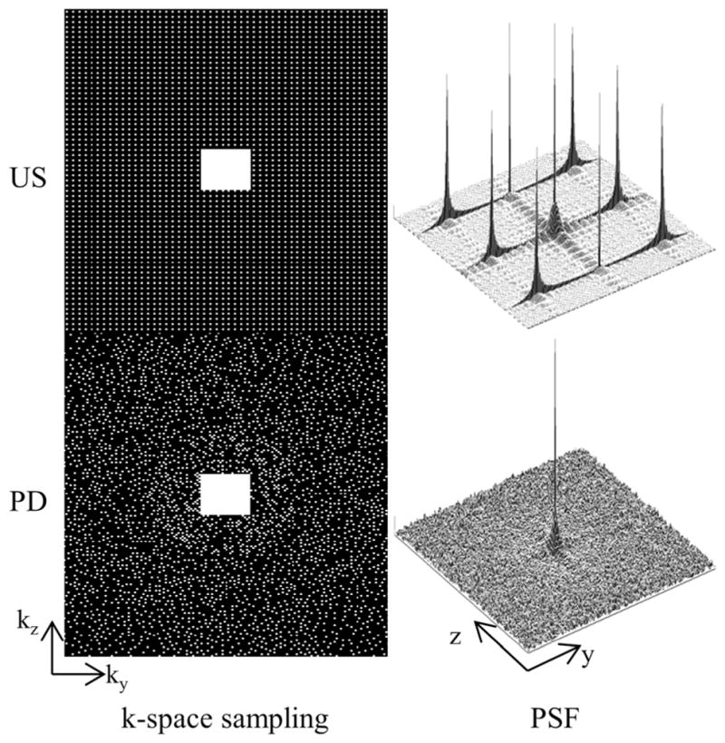
Uniformly undersampled (US) and Poisson disk (PD) k-space sampling pattern and their corresponding magnitude point-spread function (PSF). Both schemes sample the central 24 × 24 region for kernel calibration and result in 7.7x acceleration. Additionally, both schemes avoid large gaps of nonsampled points in k-space, which is desirable for parallel imaging. In contrast, the PSF of the Poisson disk pattern suggests that aliasing artifacts may appear incoherent, which is beneficial when using compressed sensing.

Signal Reconstruction

The water and fat images and the B₀ field map are estimated from the undersampled k-space measurements using parallel imaging, compressed sensing, and multiscale cubic B-splines. First, coil sensitivity maps are derived from the SPIRiT (31) k-space convolution kernel. Next, the coil-combined water and fat images and the B₀ field map are estimated in an alternating manner. The water and fat images are estimated with an l₁-regularization on their respective transform coefficients and the B₀ field map is estimated using multiscale cubic B-splines. The following subsections describe in detail the three components of the reconstruction. The components are then brought together in an algorithm that summarizes the steps of the reconstruction.

Parallel Imaging

Traditionally, a distinction in parallel imaging has been made between image-domain methods such as SENSE (21) and k-space methods such as GRAPPA (22). Recently, Lai et al. (33) and Lustig et al. (34) have addressed the superficiality of this distinction. Specifically, they have shown that the coil sensitivity maps that are used in image-domain methods can be derived from the convolution kernels that are used in k-space methods. Thus, any “k-space” parallel imaging method can be equivalently implemented as an “image-domain” method.

In this work, we use coil sensitivity maps that have been derived from the SPIRiT (31) k-space kernel. An explanation of this derivation is presented in Appendix A. Figure 2 shows the coil images and derived coil sensitivities for a liver dataset that will be presented later. Once the coil sensitivity maps have been derived, they remain fixed throughout the remainder of the reconstruction. An advantage of using the derived coil sensitivities is that the calibration consistency constraint is implicitly imposed whereas imposing this constraint in k-space would require an explicit calibration consistency expression in the reconstruction (see Eq. 10 in Ref. 31). Lai et al. (33) have shown the benefit of using the derived coil sensitivities because the absence of the explicit calibration consistency expression reduces the computational complexity of the iterative reconstruction.

FIG. 2.

The top row in each set of images shows the fully sampled coil images and the bottom row shows the corresponding coil sensitivities (magnitude) that were derived from the SPIRiT k-space kernel using only the central 16 phase encode lines. Using the coil sensitivities implicitly imposes the SPIRiT constraint, which avoids the need for an explicit calibration consistency expression in the reconstruction.

Compressed Sensing

The undersampled k-space measurements are modeled as a linear function of the coil-combined water and fat images. The linear map (F_uCΨA) is, in general, unknown because the coil sensitivity maps (C) and B₀ field map-dependent term (Ψ) are unknown. However, given an estimate of C and Ψ, the linear mapping becomes known and the water and fat images can be estimated using compressed sensing (28) by exploiting their presumed compressibility in a predetermined linear transform.

Specifically, given C and Ψ, we estimate the water and fat images via Eq. 3, where W represents the Daubechies-4 wavelet transform that operates separately on the water and fat images. We impose sparsity constraints on the coil-combined water and fat images rather than on the individual coil images because the latter potentially have less sparsity due to coil sensitivity-dependent magnitude and phase variations.

$$\underset{\mathbf{\rho }}{min}{\left|\right|{\mathbf{k}}_{\mathbf{u}}-{\mathbf{F}}_{\mathbf{u}}\mathbf{C}\mathbf{\Psi }\mathbf{A}\mathbf{\rho }\left|\right|}_2^2+\mathbf{\lambda }{\mid \mathbf{W}\mathbf{\rho }\mid }_1$$ [3]

We assume that the noise is independently and identically distributed (i.e., Σ = σ²I). The parameter λ balances data fidelity with transform sparsity and was chosen empirically based on subjective assessment of reconstructed image quality. The expression in Eq. 3 is a convex optimization problem that is solved using conjugate gradients.

Multiscale Cubic B-splines

An accurate B₀ field map is a vital prerequisite for uniform water–fat separation, however estimating this parameter is challenging due to the nonconvexity of the least-squares cost as a function of the field map value. To guide the reconstruction, the assumption of a smoothly varying B₀ field map is often made (12,15).

In this work, we propose to use multiscale cubic B-splines for B₀ field map estimation. Skare et al. have found that cubic B-splines provided a concise and accurate representation of the B₀ field inhomogeneity that arose from metallic implants (35). We extend their finding by incorporating a multiscale element (15) to avoid converging to local minima B₀ field map estimates. We first estimate a global value by restricting the B₀ field map estimate to one common value for all pixels. We then refine the field map estimate using the multiscale cubic B-splines. Figure 3 shows 2-D cubic B-spline functions and the corresponding B-spline set, from coarser to finer scale. The support size of the cubic B-spline changes by a factor of three-fourths in each dimension between successive scales. For example, the coarsest scale B-spline in Fig. 3 has a support size of 256 × 256 pixels while the support size at one finer level is 192 × 192 pixels. The B-splines are nonnegative everywhere and the sum of the functions at any spatial position is one. Details on the creation of the cubic B-spline functions and sets are presented in Appendix B.

FIG. 3.

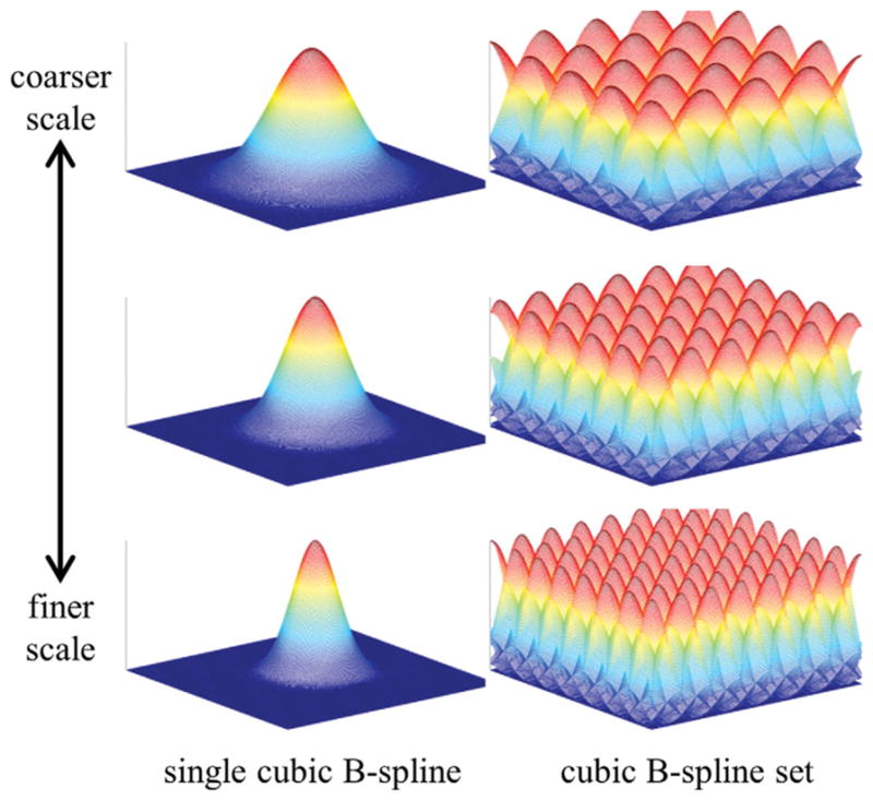
Single cubic B-spline functions from coarser scale (top) to finer scale (bottom) and their corresponding cubic B-spline sets. The B-spline set is created by spatially shifting the single cubic B-spline in both spatial directions by multiples of the knot spacing. The cubic B-splines are nonnegative everywhere and the set sums to one at all spatial positions. The field map update term at the mth scale is restricted to be in the space that is spanned by the mth cubic B-spline set.

The B₀ field map estimate is updated gradually using cubic B-splines of successively finer scales. The update expression at the mth scale is shown in Eq. 4. A full derivation appears in Appendix C.

$$\underset{\mathbf{\Delta }\mathbf{\psi },\mathbf{\Delta }\mathbf{\rho }}{min}{\left|\right|\mathbf{r}-\mathbf{x}(\mathbf{\Delta }\mathbf{\psi },\mathbf{\Delta }\mathbf{\rho })\left|\right|}_2^2+\mathbf{\lambda }{\mid \mathbf{W}\mathbf{\Delta }\mathbf{\rho }\mid }_1\text{s}.\text{t}.\mathbf{\Delta }\mathbf{\psi }\in \text{span}\{{\mathbf{B}}_{\mathbf{m}}\}$$ [4]

In Eq. 4, Δψ is the field map update term, Δρ is the error of the current water–fat image estimates, r is the residual error between the k-space measurements and the current estimate of acquired k-space, x is a linear function that relates the unknown error terms (Δψ, Δρ) to the residual, and B_m represents the cubic B-spline set at the mth scale. Upon estimating Δψ, it is added to the current field map estimate. The water–fat error term, Δρ, is discarded after estimation. The expression in Eq. 4 is a convex function of both Δψ and Δρ that is also solved using conjugate gradients.

Iterative Decomposition

The reconstruction steps are summarized in the following algorithm.

1. Derive coil sensitivities from SPIRiT k-space kernel (this will fix C)

2. Estimate global B₀ field map value, then select the coarsest-level cubic B-spline set (m = 1)

3. Estimate the water and fat images with fixed C and current Ψ (Eq. 3).

4. Estimate the B₀ field map update term (Δψ) using cubic B-splines at the current (i.e., mth) scale (Eq. 4), then add the update term to the current B₀ field map estimate (this will update Ψ)

5. IF max of |Δψ| < ε (e.g., 1 Hz)

   • Go to Step 6

   ELSE

   • Go to Step 3

6. IF current scale is equal to the predefined finest-scale

   • Done

   ELSE

   • Update cubic B-spline set to be one finer scale (m = m + 1)

   • Go to Step 3

Upon convergence, the water and fat estimates (ρ̂) and the B₀ field map estimate (ψ̂) are a local minimizer of the following cost function

$$\underset{\mathbf{\rho },\mathbf{\psi }}{min}{\left|\right|{\mathbf{k}}_{\mathbf{u}}-{\mathbf{F}}_{\mathbf{u}}\mathbf{C}\mathbf{\Psi }\mathbf{A}\mathbf{\rho }\left|\right|}_2^2+\mathbf{\lambda }{\mid \mathbf{W}\mathbf{\rho }\mid }_1\text{s}.\text{t}.\mathbf{\psi }\in \text{span}\{{\mathbf{B}}_{max}\}$$ [5]

where B_max is the set of finest-scale cubic B-splines. Note that this implies that all intermediate B₀ field map estimates are in the space spanned by B_max, which in turn implies that span{B_m} ⊆ span {B_max} for all m ≤ max.

In Vivo Experiments

Experiments were conducted with volunteer consent on a GE Signa EXCITE HDx 3-T system (GE Healthcare, Waukesha, WI) using an investigational GE IDEAL 3-D spoiled-gradient-echo sequence. Fully sampled measurements were collected at three TEs using unipolar readouts with one TE per TR and sampling bandwidth = ±125 kHz. Data were collected from the liver, brachial plexus, ankle, and knee. Table 1 lists the acquisition parameters for each of the datasets. In addition, a prospectively undersampled knee dataset was collected using a custom-built in-house sequence at 8.6x acceleration factor using the same prescription as the fully sampled knee dataset. This scan was done immediately after the fully sampled knee scan.

Table 1.

Acquisition Parameters

Anatomy	Coil	Matrix Size	FOV (cm)	Δz (mm)	TE1 (ms)	ΔTE (ms)	Scan Time (mm:ss)
Liver	Eight-channel torso	256 × 256 × 8	34	5	2.184	0.794	00:38
Brachial Plexus	Eight-channel neurovascular	192 × 192 × 64	38	2.4	2.184	0.796	04:24
Ankle	Eight-channel torso	192 × 192 × 64	24	2	2.184	0.796	04:04
Knee	Eight-channel knee	192 × 192 × 160	18	1	2.184	0.796	12:22

FOV stands for field of view, Δz represents the slice thickness, and ΔTE represents the echo time spacing. The scan time represents the time to acquire the fully sampled dataset. The prospectively undersampled knee dataset was also collected with the shown parameters at 8.6x acceleration, which reduced the scan time to 01:25.

To test the proposed approach, we retrospectively undersampled the datasets using a Poisson disk sampling pattern. Table 2 lists the size of the calibration region and the net acceleration factor that were used for each of the datasets. The coil sensitivity maps were derived from a 7 × 7 SPIRiT k-space kernel. The coarsest-scale cubic B-spline had a 1-D support size equal to the size of the corresponding image dimension (i.e., for an M × N image, the coarsest-scale B-spline was of size M × N). The support size of the B-spline functions was scaled by a factor of three-fourths in each dimension between successive scales. For example, the next coarsest-scale B-spline would be of size 3M/4 × 3N/4, followed by 9M/16 × 9N/16, and so on. The finest-scale cubic B-spline (CBS) had a 1-D support size equal to 16. The proposed approach will hereafter be referred to as PI-CS-CBS. The prospectively undersampled dataset was reconstructed in the same manner as the fully sampled dataset. The reconstruction time using the proposed approach depended on the matrix size of each slice and was typically between 15 and 30 min (24 CPUs, 2.93-GHz, 48-GB RAM).

Table 2.

Undersampling Parameters

Anatomy	Calibration Region (ky × kz)	Outer Reduction (ky × kz)	Net Acceleration
Liver	16 × N/A	4 × N/A	3.4x
Brachial Plexus	24 × 24	3 × 3	6.4x
Ankle	24 × 24	3 × 3	6.4x
Knee	24 × 24	3 × 3	7.7x/8.6x*

This table shows the size of the fully sampled calibration region, the outer reduction factor, and the net acceleration that was used to retrospectively downsample each of the datasets. The outer reduction factor is only applicable to uniform undersampling.

^*The PI-CS-CBS estimates of the knee were reconstructed from datasets that had been downsampled (retrospective and prospective) by a factor of 8.6x.

To compare our approach, we implemented an existing parallel imaging and water–fat separation approach. The fully sampled data were uniformly undersampled using the parameters listed in Table 2. The retrospectively undersampled k-space data were then reconstructed using Autocalibrated Reconstruction for Cartesian Sampling (ARC) (36) with a 7 × 7 ARC k-space kernel. Subsequently, the data were coil combined (37) and then water–fat separation was done using IDEAL with region-growing (IDEAL-RG) (10,12). This reconstruction will hereafter be referred to as ARC/IDEAL-RG. We used the ARC implementation found in the SPIRiT software package (31). To serve as a reference, the fully sampled data were first coil combined and then passed to the IDEAL-RG reconstruction. This reconstruction will hereafter be referred to as IDEAL-RG. We also reconstructed the fully sampled brachial plexus dataset using voxel-independent IDEAL (IDEAL-VI) (38). Note that for the brachial plexus dataset, the proposed multiscale cubic B-spline approach was used in place of IDEAL-RG, because the latter technique was not able to overcome the significant off-resonance encountered in this anatomy.

RESULTS

Figure 4 shows the B₀ field map and the water and fat image estimates of the liver using 1x IDEAL-RG, 3.4x ARC/IDEAL-RG, and 3.4x PI-CS-CBS. The arrows in the ARC/IDEAL-RG estimates point to aliasing artifacts and the arrowheads highlight regions of noise amplification.

FIG. 4.

B₀ field map, water, and fat estimates of the liver using an eight-channel torso coil. The ARC/IDEAL-RG estimates exhibit unresolved aliasing artifacts (arrows) and noise amplification (arrowhead). These artifacts were anticipated because the outer acceleration factor of 4 is greater than the number of coils along the axis of undersampling. In contrast, the estimates using the proposed method exhibit only slight incoherent artifacts as a result of the Poisson disk sampling and l₁-regularization.

Figure 5 shows the B₀ field map and the water and fat image estimates of the brachial plexus using 1x IDEAL-VI, 1x CBS, 6.4x ARC/CBS, and 6.4x PI-CS-CBS. The white ellipses in the IDEAL-VI B₀ field map outline areas of incorrect estimates that cause water–fat swaps. The white arrowheads point to regions of noise amplification in the ARC/CBS estimates.

FIG. 5.

B₀ field map, water, and fat estimates of the brachial plexus using an eight-channel neurovascular coil. Field map estimate errors using IDEAL-VI (white ellipses) cause water–fat swaps. The CBS field map estimation approach correctly estimates the field map to avoid the swaps. The ARC/CBS estimates exhibit noise artifacts (arrowheads), especially in the brain. These artifacts were expected because the 3x by 3x outer acceleration factor is greater than the number of receiver elements. The estimates using the proposed PI-CS-CBS approach exhibit a relatively reduced level of artifacts. Slight loss of subtle features is seen in the PI-CS-CBS estimate (black arrow).

Figure 6 shows the B₀ field map and the water and fat image estimates of the ankle using 1x IDEAL-RG, 6.4x ARC/IDEAL-RG, and 6.4x PI-CS-CBS. The arrowheads highlight noise amplification in the ARC/IDEAL-RG estimates.

FIG. 6.

B₀ field map, water, and fat estimates of the ankle using an eight-channel torso coil. The arrowheads in the ARC/IDEAL-RG estimates indicate regions of noise amplification. The outer acceleration factor (3x by 3x) was greater than the number of receiver channels so these artifacts were expected. The estimates using the proposed PI-CS-CBS approach exhibit incoherent artifacts that appear more benign than the artifacts in the ARC/IDEAL-RG estimates.

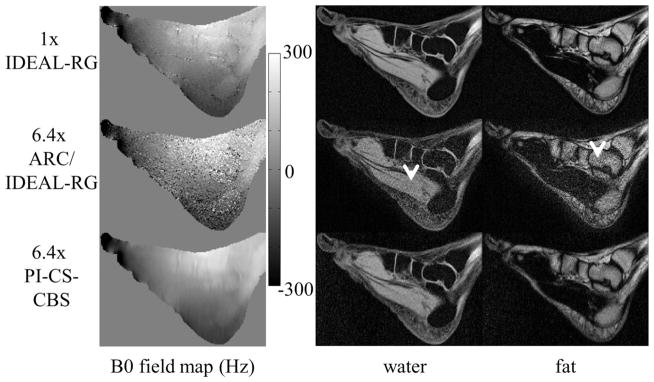
Figure 7 shows the B₀ field map and the water and fat image estimates of the knee using 1x IDEAL-RG, 7.7x ARC/IDEAL-RG (retrospective), 8.6x PI-CS-CBS (retrospective), and 8.6x PI-CS-CBS (prospective). The same Poisson disk pattern was used for the retrospective and prospective undersampling. The arrows and arrowheads in the ARC/IDEAL-RG estimates highlight, respectively, artifacts and areas of noise amplification. Both the retrospective and prospective results using the proposed method are presented to show that system issues, such as eddy currents, associated with the k-space sampling order do not affect the quality of the water–fat separation.

FIG. 7.

B₀ field map, water, and fat estimates of the knee using an eight-channel knee coil. The arrowheads and arrows in the ARC/IDEAL-RG estimates highlight, respectively, regions of noise amplification and image artifacts. These artifacts were anticipated because the outer acceleration factor of 3x by 3x is greater than the number of receiver elements. In contrast, the estimates using the proposed method exhibit incoherent artifacts as a result of the Poisson disk sampling and l₁-regularization. System issues, such as eddy currents, that are associated with the k-space sampling order do not affect the quality of the water–fat separation as evidenced by the retrospective versus prospective results.

DISCUSSION

The proposed PI-CS-CBS approach yielded water, fat, and field map estimates of better quality than ARC/IDEAL-RG. The ARC/IDEAL-RG estimates exhibited severe artifacts, which were anticipated, because the outer acceleration factor was greater than the number of coils along the dimension(s) of undersampling in all cases. In the proposed approach, the Poisson disk sampling caused incoherent aliasing artifacts that were reduced by the l₁-regularization in the reconstruction. Any remaining artifacts appeared much more benign than the structured artifacts in the ARC/IDEAL-RG estimates. The smaller number of slice encodes in the brachial plexus and ankle datasets versus the knee dataset limited the degree of wavelet compressibility along that dimension, and may have contributed to the slight loss of subtle features in the brachial plexus and ankle estimates as compared to the knee estimates.

The joint parallel imaging and compressed sensing approach imposed two complementary constraints on the reconstruction; one was based on the distinct spatial sensitivities of the receiver elements, the other on the presumed compressibility of the underlying images. By using coil sensitivities that were derived from the SPIRiT k-space kernel, we were able to impose the SPIRiT constraint without requiring an explicit calibration consistency expression in the reconstruction. The use of coil sensitivities allowed for the reconstruction of coil-combined images, which reduced the computational complexity as compared to reconstructing one set of images (i.e., water, fat, B₀ field map) for each coil. In addition, reconstructing the coil-combined images freed the sparsifying transform from the responsibility of capturing the magnitude and phase variations of the coil sensitivities.

The multiscale cubic B-splines provided an accurate and compact representation of the B₀ field map. As an example of compactness, only 4489 (= 67²) cubic B-splines were used at the finest scale to represent the B₀ field map of 65,536 (= 256 × 256) pixels in the liver dataset. This equates to a 14.6x oversampling factor, which allowed the B₀ field map to be accurately recovered from an undersampled k-space acquisition. The multiscale element gradually guided the estimate of the B₀ field map. The benefit of this approach was most apparent in the brachial plexus dataset in which the IDEAL-VI B₀ field map estimate had numerous errors that caused water–fat swaps. The estimates, from both fully sampled and undersampled data, using the cubic B-splines did not exhibit these swaps. A tradeoff when using the cubic B-splines is a smoothing of the B₀ field map estimate. We have calculated that the full-width half-maximum of the point-spread function for field map estimation is approximately eight pixels in one dimension. Empirically, this degree of smoothing does not seem to affect the quality of the water–fat separation.

The current framework has some limitations. First, the topic of quantitation has not been addressed. Accurate water–fat quantitation (19,39) requires compensation for confounding factors, the most prominent of which is $R_2^{\ast }(=1/T_2^{\ast })$. Fortunately, the signal model that we have proposed in Eq. 1 is easily amended to account for the $R_2^{\ast }$ parameter. We are currently investigating the necessary modifications to the reconstruction routine to account for this confounding factor. In addition, the effect on water–fat quantitation caused by small errors in the B₀ field map estimate using cubic B-splines must be explored. It may be that an error of only a few Hertz causes significant errors in quantitation. Second, we ignored the phase accrual during the readout due to chemical shift off-resonance (24) because its effects were minimal for the Cartesian trajectory and high sampling bandwidth that we used. If a non-Cartesian trajectory was used, one would have to account for the distinct time that each k-space point was sampled. Next, the regularization parameter λ was chosen empirically. This is acceptable for showing feasibility of the proposed method but an automated procedure would be required for wide acceptance. In addition, the reconstruction time would need to be shortened to permit online reconstruction. Lastly, the pulse sequence that we used for prospective undersampling was limited to sampling the same phase encode line for all TEs. This limitation restricted the sampling incoherence to the k_y–k_z plane rather than the k_y–k_z-TE volume. Blipping the phase encode between consecutive echoes would increase sampling incoherence, which may slightly improve results.

CONCLUSION

We have demonstrated the feasibility of integrating parallel imaging and compressed sensing for accelerated water–fat separation. In addition, we have introduced the use of multiscale cubic B-splines, which provided a compact representation and accurate estimation of the B₀ field map. The proposed approach was compared to an existing parallel imaging and water–fat separation method, and was found to yield image estimates of better quality. In all cases, the outer acceleration factor was greater than the number of coils along the dimension(s) of undersampling.

APPENDIX A

Deriving coil sensitivity maps from the SPIRiT convolution kernel

The calibration consistency expression proposed by Lustig et al. (31) is:

$${\mathbf{k}}_{\mathbf{i}}=\sum _{j=1}^{N_{\text{c}}}{\mathbf{g}}_{\mathbf{ij}}\otimes {\mathbf{k}}_{\mathbf{j}},\forall i$$ [A1]

where k_i represents the full k-space measured by the ith coil, g_ij is the convolution kernel, N_c is the number of coils, and ⊗ denotes the circular convolution operation. In words, this expression enforces the constraint that each k-space point is a weighted sum of its k-space neighbors from all coils. The weights, found in g_ij, are calculated using a fully sampled calibration region.

Taking the inverse Fourier transform of Eq. A1 yields:

$${\mathbf{I}}_{\mathbf{i}}=\sum _{j=1}^{N_{\text{c}}}{\mathbf{G}}_{\mathbf{ij}}.\ast {\mathbf{I}}_{\mathbf{j}},\forall i$$ [A2]

where I_i is the ith coil image, G_ij is the inverse Fourier transform of g_ij, and * denotes pixel-wise multiplication. Equation A2 can be written in terms of each voxel rather than for each coil image, as seen in Eq. A3.

$$\left[\begin{array}{c}{I}_1(x,y)\\ I_2(x,y)\\ .\\ .\\ I_{N_{\text{c}}}(x,y)\end{array}\right]=\left[\begin{array}{ccccc}{G}_{11}(x,y)& G_{12}(x,y)& .& .& G_{1N_{\text{c}}}(x,y)\\ G_{21}(x,y)& G_{22}(x,y)& .& .& G_{2N_{\text{c}}}(x,y)\\ .& .& .& .& .\\ .& .& .& .& .\\ G_{N_{\text{c}}1}(x,y)& G_{N_{\text{c}}2}(x,y)& .& .& G_{N_{\text{c}}{N}_{\text{c}}}(x,y)\end{array}\right]\times \left[\begin{array}{c}{I}_1(x,y)\\ I_2(x,y)\\ .\\ .\\ I_{N_{\text{c}}}(x,y)\end{array}\right]\forall x,y$$ [A3]

Notice that Eq. A3 is still a representation of the calibration consistency expression, but in a different form than Eq. A1. At this point, there is no significant difference between the two forms other than one involves a circular convolution while the other uses pixel-wise multiplication.

Let us now focus on one particular pixel and drop the pixel indices in Eq. A3 for brevity’s sake, which allows us to concisely write Eq. A3 as:

$$\mathbf{v}=\mathbf{Hv}$$ [A4]

According to Eq. A4, the calibration consistency expression says that v should be in the space that is spanned by the eigenvectors of H that have associated eigenvalue equal to one. With no FOV overlap, Lai et al. (33) have shown that H will have one eigenvalue that is equal to one. In this case, v is a scaled version of e₁, which is the eigenvector with eigenvalue equal to one and where the scalar α ∈ C¹, as seen in Eq. A5.

$$\mathbf{v}=\alpha ·{\mathbf{e}}_{\mathbf{1}}$$ [A5]

The following equation can also be written for v (still omitting subscripts):

$$\mathbf{v}=\left[\begin{array}{c}{I}_1\\ I_2\\ .\\ .\\ I_{N_{\text{c}}}\end{array}\right]=m·\left[\begin{array}{c}{C}_1\\ C_2\\ .\\ .\\ C_{N_{\text{c}}}\end{array}\right]$$ [A6]

where m is the magnetization and C_i denotes coil sensitivity value of the ith coil. Equating the terms in Eqs. A5 and A6, we see that e₁ contains the coil sensitivities.

APPENDIX B

Cubic B-Splines

A 1-D cubic B-spline is defined as:

$$b(t)=\{\begin{array}{ll}\frac{2}{3}-(1-\frac{\mid t\mid }{2})t^2\hfill & 0\le \mid t\mid \le 1\hfill \\ \frac{{(2-\mid t\mid )}^3}{6}\hfill & 1<\mid t\mid \le 2\hfill \\ 0\hfill & \text{else}\hfill \end{array}$$ [B1]

This function is nonzero only on the interval (−2, 2). To create the base 1-D cubic B-spline, b(t) is uniformly sampled on the interval (−2, 2) such that the number of sampled points equals the desired support size s (e.g., 128 pixels). A knot spacing, h_t, is defined as:

$$h_t=\text{round}\left(\frac{s-1}{4}\right)$$ [B2]

To create a base 2-D cubic B-spline of size M × N, two cubic B-splines, one with length M and the other with length N, and their associated knot spacing are first calculated. The base 2-D cubic B-spline is then created via an outer product of the two 1-D cubic B-spline functions. The 2-D cubic B-spline set is created by spatially shifting the base 2-D cubic B-spline by all combinations of the multiples (both positive and negative) of the knot spacing in both dimensions. For a I × J (e.g., 256 × 192 pixels) field map, the base 2-D cubic B-spline is shifted in both dimensions until it is entirely zero in the I × J image. Shifting by the knot spacing ensures that the sum of the B-spline set at any spatial position is equal to one. The creation of a base cubic B-spline and associated set in higher dimensions can be done using a straightforward extension of the 2-D example presented here.

APPENDIX C

B₀ Field Map Update

To derive the expression for the B₀ field map update (Δψ), we begin by rewriting the signal model (also found in Eq. 2)

$${\mathbf{k}}_{\mathbf{u}}={\mathbf{F}}_{\mathbf{u}}\mathbf{C}\mathbf{\Psi }\mathbf{A}\mathbf{\rho }+\mathbf{N}(0,\mathbf{\sum })$$ [C1]

The unknown terms at this stage are the B₀ field mapdependent term (Ψ) and the water and fat images (ρ). However, we have current estimates for both of the terms, which we use to rewrite Eq. C1 as:

$${\mathbf{k}}_{\mathbf{u}}={\mathbf{F}}_{\mathbf{u}}\mathbf{C}(\widehat{\mathbf{\Psi }}·\mathbf{\Delta }\mathbf{\Psi })\mathbf{A}(\widehat{\mathbf{\rho }}+\mathbf{\Delta }\mathbf{\rho })+\mathbf{N}(0,\mathbf{\sum })$$ [C2]

where, for example, ρ̂ denotes the current (known) water and fat estimates and Δρ represents the error (unknown) in the estimate. The same convention is used for the B₀ field map-dependent term. Taking the first-order Taylor approximation for the exponential terms in Δψ results in

$${\mathbf{k}}_{\mathbf{u}}={\mathbf{F}}_{\mathbf{u}}\mathbf{C}(\widehat{\mathbf{\Psi }}·\mathbf{\Delta }\mathbf{T})\mathbf{A}(\widehat{\mathbf{\rho }}+\mathbf{\Delta }\mathbf{\rho })+\mathbf{N}(0,\mathbf{\sum })$$ [C3]

where ΔT is a block diagonal matrix that contains 1 = j2π Δψ^pt_n on the pth diagonal of the nth block, where Δψ^p is the field map update term at the pth pixel and t_n is the time of the nth echo.

At this point, Eq. C3 is modified by grouping the known terms on the left-hand side, the unknown terms on the right-hand side, and discarding the ΔS·Δρ term where ΔS is a block diagonal matrix that contains j2π Δψ^pt_n on the pth diagonal of the nth block.

$${\mathbf{k}}_{\mathbf{u}}-{\mathbf{F}}_{\mathbf{u}}\mathbf{C}\widehat{\mathbf{\Psi }}\mathbf{A}\widehat{\mathbf{\rho }}={\mathbf{F}}_{\mathbf{u}}\mathbf{C}\widehat{\mathbf{\Psi }}\mathbf{\Delta }\mathbf{SA}\widehat{\mathbf{\rho }}+{\mathbf{F}}_{\mathbf{u}}\mathbf{C}\widehat{\mathbf{\Psi }}\mathbf{A}\mathbf{\Delta }\mathbf{\rho }+\mathbf{N}(0,\mathbf{\sum })$$ [C4]

Notice that the left-hand side of Eq. C4 is the residual error between the measurements and the current estimate while the right-hand side is a function of the errors in the water, fat, and B₀ field map estimates as well as noise. Denoting the left-hand side of Eq. C4 as r, the right-hand side as x(Δψ, Δρ), and assuming that the noise is independently and identically distributed (i.e., Σ = σ²I), we arrive at the expression for the B₀ field map update in the mth cubic B-spline set.

$$\underset{\mathbf{\Delta }\mathbf{\psi },\mathbf{\Delta }\mathbf{\rho }}{min}{\left|\right|\mathbf{r}-\mathbf{x}(\mathbf{\Delta }\mathbf{\psi },\mathbf{\Delta }\mathbf{\rho })\left|\right|}_2^2+\mathbf{\lambda }{\mid \mathbf{W}\mathbf{\Delta }\mathbf{\rho }\mid }_1\text{s}.\text{t}.\mathbf{\Delta }\mathbf{\psi }\in \text{span}\{{\mathbf{B}}_{\mathbf{m}}\}$$ [C5]

The Δρ term does not need to be estimated but we have found that doing so speeds the convergence of the estimate of Δψ. The Δρ term is discarded after estimation.

References

- 1.Kellman P, Hernando D, Shah S, Zuehlsdorff S, Jerecic R, Mancini C, Liang ZP, Arai AE. Multiecho Dixon fat and water separation method for detecting fibrofatty infiltration in the myocardium. Magn Reson Med. 2009;61:215–221. doi: 10.1002/mrm.21657. [DOI] [PMC free article] [PubMed] [Google Scholar]
- 2.Alabousi A, Al-Attar S, Joy TR, Hegele RA, McKenzie CA. Evaluation of adipose tissue volume quantification with IDEAL fat-water separation. J Magn Reson Imaging. 2011;34:474–479. doi: 10.1002/jmri.22603. [DOI] [PubMed] [Google Scholar]
- 3.McMahon CJ, Madhuranthakam AJ, Wu JS, Yablon CM, Wei JL, Rofsky NM, Hochman MG. High-resolution proton density weighted three-dimensional fast spin echo (3D-FSE) of the knee with IDEAL at 1. 5 tesla: comparison with 3D-FSE and 2D-FSE—initial experience. J Magn Reson Imaging. 2012;35:361–369. doi: 10.1002/jmri.22829. [DOI] [PubMed] [Google Scholar]
- 4.Low RN, Austin MJ, Ma J. Fast spin-echo triple echo Dixon: initial clinical experience with a novel pulse sequence for simultaneous fat-suppressed and nonfat-suppressed T2-weighted spine magnetic resonance imaging. J Magn Reson Imaging. 2011;33:390–400. doi: 10.1002/jmri.22453. [DOI] [PubMed] [Google Scholar]
- 5.Haase A, Frahm J, Hanicke W, Matthaei D. 1H NMR chemical shift selective (CHESS) imaging. Phys Med Biol. 1985;30:341–344. doi: 10.1088/0031-9155/30/4/008. [DOI] [PubMed] [Google Scholar]
- 6.Bley TA, Wieben O, Francois CJ, Brittain JH, Reeder SB. Fat and water magnetic resonance imaging. J Magn Reson Imaging. 2010;31:4–18. doi: 10.1002/jmri.21895. [DOI] [PubMed] [Google Scholar]
- 7.Dixon WT. Simple proton spectroscopic imaging. Radiology. 1984;153:189–194. doi: 10.1148/radiology.153.1.6089263. [DOI] [PubMed] [Google Scholar]
- 8.Glover GH, Schneider E. Three-point Dixon technique for true water/fat decomposition with B0 inhomogeneity correction. Magn Reson Med. 1991;18:371–383. doi: 10.1002/mrm.1910180211. [DOI] [PubMed] [Google Scholar]
- 9.Xiang QS, An L. Water-fat imaging with direct phase encoding. J Magn Reson Imaging. 1997;7:1002–1015. doi: 10.1002/jmri.1880070612. [DOI] [PubMed] [Google Scholar]
- 10.Reeder SB, Pineda AR, Wen Z, Shimakawa A, Yu H, Brittain JH, Gold GE, Beaulieu CH, Pelc NJ. Iterative decomposition of water and fat with echo asymmetry and least-squares estimation (IDEAL): application with fast spin-echo imaging. Magn Reson Med. 2005;54:636–644. doi: 10.1002/mrm.20624. [DOI] [PubMed] [Google Scholar]
- 11.Ma J. Breath-hold water and fat imaging using a dual-echo two-point Dixon technique with an efficient and robust phase-correction algorithm. Magn Reson Med. 2004;52:415–419. doi: 10.1002/mrm.20146. [DOI] [PubMed] [Google Scholar]
- 12.Yu H, Reeder SB, Shimakawa A, Brittain JH, Pelc NJ. Field map estimation with a region growing scheme for iterative 3-point water-fat decomposition. Magn Reson Med. 2005;54:1032–1039. doi: 10.1002/mrm.20654. [DOI] [PubMed] [Google Scholar]
- 13.Lu W, Hargreaves BA. Multiresolution field map estimation using golden section search for water-fat separation. Magn Reson Med. 2008;60:236–244. doi: 10.1002/mrm.21544. [DOI] [PubMed] [Google Scholar]
- 14.Jacob M, Sutton BP. Algebraic decomposition of fat and water in MRI. IEEE Trans Med Imaging. 2009;28:173–184. doi: 10.1109/TMI.2008.927344. [DOI] [PubMed] [Google Scholar]
- 15.Tsao J, Jiang Y. Hierarchical IDEAL: Robust Water-Fat Separation at High Field by Multiresolution Field Map Estimation. Proceedings of the 16th Annual Meeting of ISMRM; Toronto, Canada. 2008. p. 653. [Google Scholar]
- 16.Hernando D, Kellman P, Haldar JP, Liang ZP. Robust water/fat separation in the presence of large field inhomogeneities using a graph cut algorithm. Magn Reson Med. 2010;63:79–90. doi: 10.1002/mrm.22177. [DOI] [PMC free article] [PubMed] [Google Scholar]
- 17.Berglund J, Johansson L, Ahlstrom H, Kullberg J. Three-point Dixon method enables whole-body water and fat imaging of obese subjects. Magn Reson Med. 2010;63:1659–1668. doi: 10.1002/mrm.22385. [DOI] [PubMed] [Google Scholar]
- 18.Eggers H, Brendel B, Duijndam A, Herigault G. Dual-echo Dixon imaging with flexible choice of echo times. Magn Reson Med. 2011;65:96–107. doi: 10.1002/mrm.22578. [DOI] [PubMed] [Google Scholar]
- 19.Hines CDG, Frydrychowicz A, Hamilton A, Tudorascu DL, Vigen KK, Yu H, McKenzie CA, Sirlin CB, Brittain JH, Reeder SB. T1 independent, corrected chemical shift based fat-water separation with multi-peak fat spectral modeling is an accurate and precise measure of hepatic steatosis. J Magn Reson Imaging. 2011;33:873–881. doi: 10.1002/jmri.22514. [DOI] [PMC free article] [PubMed] [Google Scholar]
- 20.Yu H, McKenzie CA, Shimakawa A, Vu AT, Brau ACS, Beatty PJ, Pineda AR, Brittain JH, Reeder SB. Multiecho reconstruction for simultaneous water-fat decomposition and estimation. J Magn Reson Imaging. 2007;26:1153–1161. doi: 10.1002/jmri.21090. [DOI] [PubMed] [Google Scholar]
- 21.Pruessmann KP, Weiger M, Scheidegger MB, Boesiger P. SENSE: sensitivity encoding for fast MRI. Magn Reson Med. 1999;42:952–962. [PubMed] [Google Scholar]
- 22.Griswold MA, Jakob PM, Heidemann RM, Nittka M, Jellus V, Wang J, Kiefer B, Haase A. Generalized autocalibrating partially parallel acquisitions (GRAPPA) Magn Reson Med. 2002;47:1202–1210. doi: 10.1002/mrm.10171. [DOI] [PubMed] [Google Scholar]
- 23.Reeder SB, Hargreaves BA, Yu H, Brittain JH. Homodyne reconstruction and IDEAL water-fat decomposition. Magn Reson Med. 2005;54:586–593. doi: 10.1002/mrm.20586. [DOI] [PubMed] [Google Scholar]
- 24.Brodsky EK, Holmes JH, Yu H, Reeder SB. Generalized k-space decomposition with chemical shift correction for non-Cartesian water-fat imaging. Magn Reson Med. 2008;59:1151–1164. doi: 10.1002/mrm.21580. [DOI] [PubMed] [Google Scholar]
- 25.Bornert P, Koken P, Eggers H. Spiral water-fat imaging with integrated off-resonance correction on a clinical scanner. J Magn Reson Imaging. 2010;32:1262–1267. doi: 10.1002/jmri.22336. [DOI] [PubMed] [Google Scholar]
- 26.Doneva M, Bornert P, Eggers H, Mertins A, Pauly J, Lustig M. Compressed sensing for chemical shift-based water-fat separation. Magn Reson Med. 2010;64:1749–1759. doi: 10.1002/mrm.22563. [DOI] [PubMed] [Google Scholar]
- 27.Sharma SD, Hu HH, Nayak KS. Accelerated water-fat imaging using restricted subspace field map estimation and compressed sensing. Magn Reson Med. 2012;67:650–659. doi: 10.1002/mrm.23052. [DOI] [PMC free article] [PubMed] [Google Scholar]
- 28.Lustig M, Donoho D, Pauly JM. Sparse MRI: the application of compressed sensing for rapid MR imaging. Magn Reson Med. 2007;58:1182–1195. doi: 10.1002/mrm.21391. [DOI] [PubMed] [Google Scholar]
- 29.Yu H, Shimakawa A, McKenzie CA, Brodsky E, Brittain JH, Reeder SB. Multiecho water-fat separation and simultaneous estimation with multifrequency fat spectrum modeling. Magn Reson Med. 2008;60:1122–1134. doi: 10.1002/mrm.21737. [DOI] [PMC free article] [PubMed] [Google Scholar]
- 30.Candes EJ, Romberg J. Sparsity and incoherence in compressive sampling. Inverse Problems. 2006;23:969–985. [Google Scholar]
- 31.Lustig M, Pauly JM. SPIRiT: iterative self-consistent parallel imaging reconstruction from arbitrary k-space. Magn Reson Med. 2010;64:457–471. doi: 10.1002/mrm.22428. [DOI] [PMC free article] [PubMed] [Google Scholar]
- 32.Cook RL. Stochastic sampling in computer graphics. ACM Trans Graph. 1986;5:51–72. [Google Scholar]
- 33.Lai P, Lustig M, Vasanawala SS, Brau AC. ESPIRiT (Efficient Eigenvector-Based L1SPIRiT) for Compressed Sensing Parallel Imaging—Theoretical Interpretation and Improved Robustness for Overlapped FOV Prescription. Proceedings of the 19th Annual Meeting of ISMRM; Montreal, Canada. 2011. p. 65. [Google Scholar]
- 34.Lustig M, Lai P, Murphy M, Vasanawala SM, Elad M, Zhang J, Pauly J. An Eigen-Vector Approach to Autocalibrating Parallel MRI, Where SENSE Meets GRAPPA. Proceedings of the 19th Annual Meeting of ISMRM; Montreal, Canada. 2011. p. 479. [Google Scholar]
- 35.Skare S, Andersson JLR. Correction of MR image distortions induced by metallic objects using a 3D cubic B-spline basis set: application to stereotactic surgical planning. Magn Reson Med. 2005;54:169–181. doi: 10.1002/mrm.20528. [DOI] [PubMed] [Google Scholar]
- 36.Beatty PJ, Brau AC, Chang S, Joshi SM, Michelich CR, Bayram E, Nelson TE, Herfkens RJ, Brittain JH. A method for autocalibrating 2-D accelerated volumetric parallel imaging with clinically practical reconstruction times. Proceedings of the 15th Annual Meeting of ISMRM; Berlin, Germany. 2007. p. 1749. [Google Scholar]
- 37.Walsh DO, Gmitro AF, Marcellin MW. Adaptive reconstruction of phased array MR imagery. Magn Reson Med. 2000;43:682–690. doi: 10.1002/(sici)1522-2594(200005)43:5<682::aid-mrm10>3.0.co;2-g. [DOI] [PubMed] [Google Scholar]
- 38.Reeder SB, Wen Z, Yu H, Pineda AR, Gold GE, Markl M, Pelc NJ. Multicoil Dixon chemical species separation with an iterative leastsquares estimation method. Magn Reson Med. 2004;51:35–45. doi: 10.1002/mrm.10675. [DOI] [PubMed] [Google Scholar]
- 39.Bydder M, Yokoo T, Hamilton G, Middleton MS, Chavez AD, Schwimmer JB, Lavine JE, Sirlin CB. Relaxation effects in the quantification of fat using gradient echo imaging. Magn Reson Imaging. 2008;26:347–359. doi: 10.1016/j.mri.2007.08.012. [DOI] [PMC free article] [PubMed] [Google Scholar]