

Abstract
Airway diseases (e.g., asthma, emphysema, and chronic bronchitis) are extremely common worldwide. Any morphological variations (abnormalities) of airways may physically change airflow and ultimately affect the ability of the lungs in gas exchange. In this study, we describe a novel algorithm aimed to automatically identify airway walls depicted on CT images. The underlying idea is to place a three-dimensional (3D) surface model within airway regions and thereafter allow this model to evolve (deform) under predefined external and internal forces automatically to the location where these forces reach a state of balance. By taking advantage of the geometric and the density characteristics of airway walls, the evolution procedure is performed in a distance gradient field and ultimately stops at regions with the highest contrast. The performance of this scheme was quantitatively evaluated from several perspectives. First, we assessed the accuracy of the developed scheme using a dedicated lung phantom in airway wall estimation and compared it with the traditional full-width at half maximum (FWHM) method. The phantom study shows that the developed scheme has an error ranging from 0.04 mm to 0.36 mm, which is much smaller than the FWHM method with an error ranging from 0.16 mm to 0.84 mm. Second, we compared the results obtained by the developed scheme with those manually delineated by an experienced (>30 years) radiologist on clinical chest CT examinations, showing a mean difference of 0.084 mm. In particular, the sensitivity of the scheme to different reconstruction kernels was evaluated on real chest CT examinations. For the ‘lung’, ‘bone’ and ‘standard’ kernels, the average airway wall thicknesses computed by the developed scheme were 1.302 mm, 1.333 mm and 1.339 mm, respectively. Our preliminary experiments showed that the scheme had a reasonable accuracy in airway wall estimation. For a clinical chest CT examination, it took around 4 minutes for this scheme to identify the inner and outer airway walls on a modern PC.
1. INTRODUCTION
Airway wall remodeling has been widely regarded as an indicator of the severity of airway diseases (e.g., chronic obstructive pulmonary disease (COPD)) in clinical practice (Bousquet et al., 2000; Berger et al., 2005). The availability of high-resolution computed tomography (CT) makes it possible to non-invasively investigate the underlying mechanism of airway remodeling by directly measuring airway wall thickness. In early days, airway wall measurement was performed manually by properly adjusting image intensity values using window levels (Webb et al., 1984; Bankier et al., 1996; Okazawa et al. 1996); however, this is a very time-consuming and error-prone process due to the large number of images involved in a single CT examination and the unavoidable perturbation associated with manual tracing. Hence, it is desirable to develop a computational tool to aid an accurate, consistent, and efficient identification of airway wall.
In the past, a number of computerized schemes have been developed to identify airway wall. A widely referred approach is the full-width at half maximum (FWHM) method (Nakano et al., 2000). It shoots a number of rays oriented from the centers of airway lumen out to the parenchyma and then estimates inner and outer wall locations by studying the intensity profile along the path of the ray (Nakano et al., 2000). The FWHM method assumes that outer and inner airway walls are located at the halfway between the local minimum in lumen or parenchyma and the maximum within airway wall, respectively. However, this method depends directly on the gray-scale profile on a ray, which may be affected by various factors such as partial volume effect or blurring effects introduced by reconstruction methods and orientation of the airways, thus leading to a potential overestimation of airway wall measures (Nakano et al., 2002; Reinhardt et al., 1997). To reduce the dependency on luminance variations, (Saragaglia et al., 2005) developed a method based on mathematical morphology and energy-based contour matching. This algorithm identifies outer airway wall in a slice-by-slice manner by progressively extending an initial closed contour (e.g., a set of connected pixels) until a predefine energy is achieved at an equilibrium state. Alternatively, (Reinhardt et al., 1997) developed a two-dimensional (2D) model-based method to estimate airway inner and outer walls by matching a predicted ray profile with an actual profile observed in available dataset. The developed model is to simulate the scanning process of an ideal airway by estimating the parameters of 2D point-spread functions (PSF) of a scanner. In implementation, it assumes that airways are circular and their axes are perpendicular to the scanning plane. If airways are scanned off-axis, the model may lead to obvious errors in measurement. In order to overcome the limitation of the method described in (Reinhardt et al., 1997). (Saba et al., 2003) used an elliptical model instead of a circular model and a full three-dimensional (3D) PSF instead of a 2D PSF. A direct least square approach is firstly used to fit inner and outer airway walls as ellipses and a tilt angle is then estimated using the major and minor axes of these ellipses. This improved strategy allows for measuring the wall thickness of airways oriented to the scan plane but has relatively high computational cost. Unlike the methods that depended on a specific model of the airway (e.g., a circular or elliptical model) or a specific function of a scanner (e.g., PSF), (San Jose Estépar et al., 2006) proposed to use phase congruency to detect inner and outer airway walls. This approach takes advantages of two facts: (1) phase congruency is present at the scanner level when reconstructing image data with different reconstruction kernels, and (2) phase congruency is a normalized measure of phase variance across scales and appears as a smooth function with local maxima in locations where local phase is consistent across scales. Due to its 2D characteristic, the identified airway walls are not smooth in 3D space. Recently, (Ortner et al., 2010, 2011) developed a 3D deformation approach for airway wall segmentation based on a generalized gradient vector flow (GGVF) (Xu and Prince, 1998). This approach (Orter et al., 2010, 2011) requires a balloon force (Cohen, 1991) based on the image intensity to prohibit the surface stopping at the inner surface of airway wall. Whereas the image intensity of airway wall may vary a lot, it is difficult for this approach to select a constant parameter for the balloon force. In addition, a Laplacian of Gaussian algorithm (Montaudon et al. 2007) and an integral based closed-form solution (Weinheimer et al., 2008) were proposed to estimate the airway thickness. In the integral based close-form solution, (Weinheimer et al. 2008) used 10% level of the rising edge and the 10% level of the trailing edge as start and end point of the integral paths. The closed form solution was implemented by solving a linear system with three variables, which corresponds to lumen, airway wall, and parenchyma, respectively.
In this study, we proposed a full automated approach to identify airway wall using an active surface model that evolved in a force field without any balloon force. By taking advantage of the geometric and density characteristics of airway wall depicted on CT images, this approach enables a 3D surface (contour) to evolve automatically to the border with the highest contrast in a distance gradient field. A detailed description of the proposed scheme and the preliminary assessment of its performance from different perspectives follow.
2. METHODS
2.1. Scheme overview
In this study, we proposed to identify airway walls depicted in a CT examination using a 3D active surface evolution approach. The underlying idea is to place a 3D surface model in a vector field and allow this model to evolve (deform) automatically under external and internal forces until these forces reach a state of balance (Figure 1). Simply switching the external energy function will lead to the identification of either inner or outer airway wall.
Figure 1.
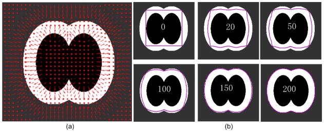
Illustration of the developed active surface model evolution approach using a 2D artificial example. This example simulates the region at the bifurcation location of an airway tree. The innermost black region, the middle white region, and outmost gray region denote respectively the airway lumen, the airway wall, and the parenchyma. (a) shows an external forced field Fext indicated by the arrows (in red). (b) shows the evolutions of the original model or contour (in purpose) at different iterations (i.e., 0, 20, 50, 100, 150, and 200).
Mathematically, given a geometric surface X(u, s) = [x(u, s), y(u, s), z(u, s)], the objective of this active surface evolution is To Whom It May Concern: minimize an energy function:
| (1) |
where X(u, s) denotes a 3D surface model, Eext denotes an external energy function, Eint denotes an internal energy function, and γ denotes the contribution of Eext to E(X). The external energy function forms a static external force field in space, which drives the surface to the location with the highest contrast. The internal energy function forms an elastic force to enforce the neighbor points having the same distance to the airway lumen. The energy minimization of E(X) will lead to the identification of the balanced state or boundary position that corresponds to the location of airway outer/inner wall.
Given a chest CT examination, this scheme consists of three steps in implementation (Figure 2). The first step is to automatically identify the airway tree depicted in the CT examination. Thereafter, three procedures are performed on the identified airway tree to define the initial surface model, the external energy function, and the internal energy function. The external energy function is computed based on the distance gradient field of the airway tree, while the internal energy function is computed based on the cross-section of the airway tree. Finally, the obtained surface model evolves under the external and internal force fields, thereby leading to the inner/outer airway wall. A detailed description of the implementation of the developed scheme follows.
Figure 2.
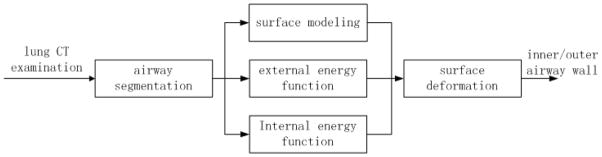
A flowchart illustrating the implementation of the developed scheme.
2.2. Initial surface model
The initial deformation surface model could be any surface or contour that is located within the airway regions. Whereas the airway lumen has a relatively higher contrast with the airway wall, we simply use the inner surface of an airway wall (i.e., airway lumen surface) as the initial model that can be obtained by any available airway segmentation approach (Sonka et al., 1996; Park et al., 1998; Aykac et al., 2003; Tschirren et al., 2005; Granham et al., 2010; van Ginneken et al., 2008). Here, we use the airway lumen identified by a previously developed airway segmentation approach (Pu et al., 2011) as the initial deformation model. The marching cubes algorithm (MCA) (Lorensen et al., 1987) is used to represent identified airway lumen as a triangle surface model, which is formed by Nv vertices . Figure 3 shows an example where the lumen region of an airway tree is modeled as a triangle mesh surface, and this model is used as the initial surface for evolution purpose.
Figure 3.
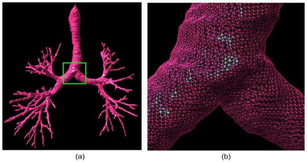
An example showing an airway tree identified by the algorithm in (Pu et al., 2011) and its triangle surface representation. (b) shows the local enlargement of the region indicated by the box in (a).
2.3. External energy function Eext
Considering that the boundaries of airway walls are regions with a high intensity contrast, namely a large difference in intensity between neighboring voxels, we define the external energy function Eext(X) in a way so that the evolution (deformation) surface will stop at locations with the largest image gradient along the distance gradient field. Figure 4 shows the procedures of computing the external energy function using an artificial example.
Figure 4.
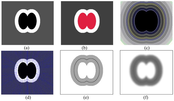
Illustration of the steps in computing the external energy function using an artificial example. (a) shows the original image I, where the internal dark region indicates the airway lumen, the bright region indicates the airway wall, and the gray region indicates the background, (b) shows the identified lumen region in red, (c) shows the distance map D, (d) shows the distance gradient field V, (e) shows the image gradient H, and (f) shows the external energy field Eext (X).
2.3.1 Narrow-band technique
In order to efficiently compute distance field and gradients, we use a narrow-band technique, by which the voxels on CT images are classified into three categories, namely “airway lumen voxels” (i.e., voxels forming the airway lumen) denoted by A, “narrow-band voxels” (i.e., voxels within a certain distance dband to airway lumen) denoted by B, and “other voxels” (i.e., remaining voxels that are far away from airway lumen) denoted by C. Thus, we have A ∩ B = A ∩ C = B ∩ C = φ and A ∪ B ∪ C = P, where P denotes all voxels on CT images. In order to identify airway wall, dband should be set at a value larger than airway wall thickness (e.g., dband = 8 mm). Whereas there is no need to compute the gradients and the distance fields on C, the computational complexity in both spatial and temporal domains may be significantly reduced with the aid of the narrow-band technique.
2.3.2 Distance map (D)
On the basis of the image voxel classification strategy mentioned in 2.3.1 (i.e., A, B, and C), we defined a distance function ϕ(p) as Eq. (2).
| (2) |
where is the smallest Euclidean distance between voxel p and the airway lumen A. We note that the distance function near the lumen (0 < ϕ(p) < dsmooth, e.g., dsmooth = 3mm) may be discontinuous due to the discrete characteristic of an image, where dsmooth < dband. Let B* ={p|0 < ϕ(p) < dsmooth}, then B* is a subset of the narrow band B, i.e., B* ⊂ B. A potential solution to this discontinuous issue is to subdivide the voxels and then compute the distance field. However, this subdivision approach has a very high computational complexity in both spatial and temporal domains. Here, we initialize the distance function as D0 = ϕ. Then we fix the distance function over region P\B* and redefine D over region B* using a Laplacian smoothing operation by minimizing
| (3) |
The discretization of (3) can be written as,
| (4) |
Eq. (4) is a convex problem, thus its optimal solution can be found iteratively. For D at each point D(x, y, z), we have
| (5) |
According to Eq. (5), we can update Dt(p) if p = (x, y, z)T ∈ B* using
| (6) |
The impact of this smoothing operation on the distance function is illustrated by a two-dimensional (2D) example in Figure 5.
Figure 5.
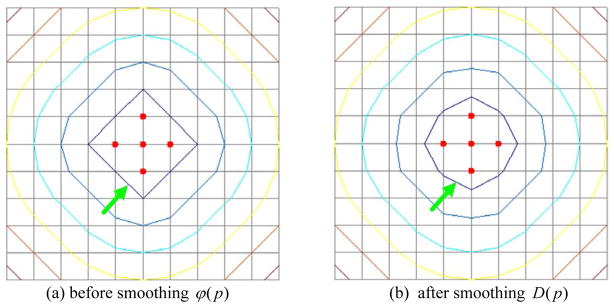
Impact of the smoothing operation mentioned in Section 2.3.2 on the computation of distance functions (maps). The red points denote the feature points when computing the distance field. The points on each contour have the same distance value. (a) shows the Euclidean distance field, ϕ(p) and (b) shows the smoothed distance field D(p).
2.3.3 Distance gradient field V
Given the region B (the narrow band) defined in section 2.3.1, the gradient field V(p) of the distance map D(p) over B is computed using
| (7) |
For the voxels in A, V(p) does not exist because the distance function equals zero everywhere. However, a similar strategy as in Section 2.3.2 can be used to obtain the vector field of A. First, the vector field V(A) is initialized by V0(A) = 0 and then updated using
| (8) |
For the sake of convenience, the vector field V is normalized, i.e., .
2.3.4 Image gradient H along the distance gradient field V
In order to generate an external force field that may lead the initial surface model to evolve progressively to airway wall boundaries, we propose to compute the signed image gradient H(p) along the distance gradient field V. We note that the distance gradient vector and the image gradient vector ∇I have the same direction at the inner airway wall boundaries, while they have opposite directions at the outer airway wall boundaries. In order to distinguish the inner and outer airway wall surfaces, H(p) needs to be computed for inner and outer airway wall surfaces respectively. When identifying outer airway wall, Houter(p) is computed as
| (9) |
where , and I denotes the intensity of CT images. H(p) is regularized by 1 over A and C to reduce the computational cost and at the same time the surface deformation is performed within region B.
When identifying inner airway wall, Hinner(p) is computed as
| (10) |
We note that when computing the image derivatives, the linear interpolation was used in this study. Hence, the scale parameters could be any value that is smaller than the voxel size, and the results will remain the same due to the linear interpolation characteristics. In our study, we simply set the scale parameter (dx) of image derivatives at 0.001 mm, which is much smaller than the CT resolution.
2.3.5 External energy function Eext
Given the image gradient H along the distance gradient field V, the external energy function of the evolution is defined as
| (11) |
where Gσ denotes Gaussian smoothing kernel with a standard deviation σ. The objective of the Gaussian filter is to improve the robustness of the scheme against image noise and/or artifacts. A large σ may significantly reduce image noises but at the same time may blur the image significnatly as well, thereby potentially introducing large errors in quantitative assessment. In our study, the value of σ is consistently set at 0.5 mm, which was determined by investigating its impact on the accuracy in airway wall thickness estimation using a lung phantom. A detailed desciripton of determining the value of σ is provided in the discussion section. The external energy is generic and can be used for the identification of either outer or inner airway wall. For outer wall identification, H = Houter and the evolution stops at the locations where the signed image gradients (from airway wall to parenchyma) are minimal; while for inner wall identification, H = Hinner and the evolution stops at the locations where the signed image gradients (from airway lumen to airway wall) are maximal.
An artificial example in Figure 6 is used to explain why we let the outer wall surface model evolve in the signed image gradient field Houter(p). As shown in Figure 6(d), for the negative gradient magnitude −M, there are two local minimum values corresponding to the inner and the outer wall, respectively. It does mean that the evolution may stop at the inner wall “N”. In contrast, as shown in Figure 6(c), the deformation will evolve from the inner wall “N” to the outer wall “O”, because there is only one local minimum value located at the outer wall. Similarly, when changing the sign of the image gradient H, the deformation will evolve to the inner wall “N”.
Figure 6.
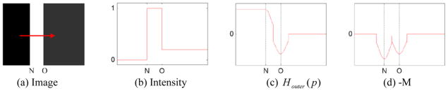
Illustration of the characteristics of the signed image gradient field Houter. (a) shows an artificial image I, where “N” indicates the inner wall, and “O” indicates the outer wall. The arrow indicates the direction of the distance gradient field V. (b) shows the image intensity profile of I along the horizontal direction from left to right, (c) shows the signed image gradient Houter along the distance gradient field V, and (d) shows negative gradient magnitude (i.e., −M) of the intensity profile in (b).
2.4. Internal energy function Eint
In order to minimize the first order and/or the second order of the surface contour X(u, s) with respect to parameters u and s (Kass et al., 1987), the internal energy function is generally defined as
| (12) |
where only the first order is considered. In this study, we define a novel internal energy function
| (13) |
The first part represents the variations of the airway thickness in a neighbor area. This part acts like a Laplacian operator to make the surface smooth, where wij =1, if Xi and Xj are neighboring points (vertices); wij = 0, otherwise. The second part represents the variations of airway thickness in the cross section of airways, where D̄(Xi) is the mean thickness of a cross section. This part is to reduce the effect of the attachment with the vessels and assure that the points on a cross-section region have a similar airway wall thickness.
To compute D̄(Xi), we use the repulsive force field based approach developed by (Cornea et al., 2005) to obtain the skeleton (central axis) of airway lumen (Figure 7b). Given a vertex Xi on a triangular mesh surface representing the initial evolution model, its nearest skeleton point Sj is identified. For Sj, there are a number of vertices on the surface model that have the nearest distances to it. Here, we define a cross section ℜj (Figure 7c) as a ring-like shape with a height of 2δ, namely ℜj ={Rk | ||Sk − Sj ||<δ}. Thus, D̄(Xi) can be computed using .
Figure 7.
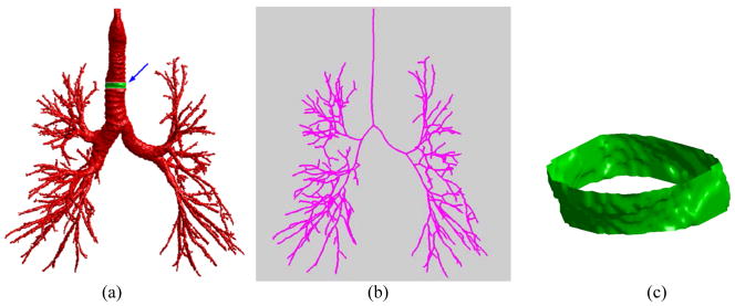
Airway skeletonization and cross section selection. (a) show an airway tree, (b) shows the skeleton of the airway tree in (a), and (c) shows the ring-like cross-section as indicated by the arrow in (a).
2.5. Surface deformation (evolution)
Given the initial surface model (a triangle mesh), the deformation (evolution) direction of each vertex Xi on this mesh is determined by the distance gradient field V(Xi) and the deformation strength is determined by both the internal and the external forces. Substituting Eq. (11) and Eq.(13) into Eq.(1) results in the final energy function
| (14) |
where the values, such as distance map D, at a non-integer point can be obtained by tri-linear interpolation.
The active surface contour that minimizes the energy function E must satisfy the Euler equation
| (15) |
which can be viewed as a force balance equation, , where the internal force Fint and the external force Fext are
| (16) |
| (17) |
where . In order to find a solution to (14), we treat X as a function of time t
| (19) |
The stabilization of Xt will lead to a solution to Eq. (14). Two artificial examples are used in Figure 8 to demonstrate the above mentioned dynamic process of the surface evolution. The example in Figure 8(a) shows the evolution of a contour in the above described external and internal force fields at the bifurcation region of an airway tree, while the example in Figure 8(b) is used to demonstrate the evolution when the airway wall is attached to other soft tissues (e.g., vessels).
Figure 8.
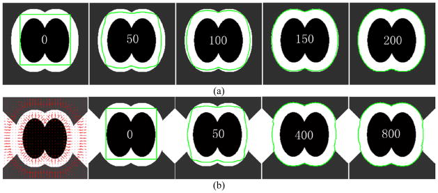
Illustration of the dynamic surface evolution under the external and internal force fields defined in this study. The dark region indicates the airways, and the bright region indicates the soft tissues (e.g., airway wall or vessels). The numbers in the middle of the images represent the time t. (a) shows the evolution of an contour (green) at the location of an airway bifurcation at different time points, and (b) shows the evolution of an contour (green) at a regions attached to soft tissues (e.g., vessels).
2.6. Performance assessment
In order to quantitatively and objectively assess the performance of the developed scheme in airway wall identification, we performed the following three experiments:
(1) A phantom study
Like many previous investigations (Reinhardt et al., 1997; Saragaglia et al., 2005; Saba et al., 2003; San Jose Estépar et al., 2006), we propose to use a dedicated commercial lung phantom manufactured by Bitica Ltd as a “reference standard” for quantitative validation purpose. This phantom has 14 tubes resembling airways and 14 tubes resembling vessels with four different radii (i.e., 1.19 mm, 1.99 mm, 2.78 mm and 3.57 mm, respectively) (Figure 9). All these tubes have the same length of 20.3 mm. The wall thickness of the airway tubes is consistently 0.79 mm. The CT examinations (Figure 10) were acquired using two different scanners (i.e., GE Lightspeed VCT and Siemens Sensation) and reconstructed using different kernels. The field of view (FOV), in-plane pixel size, and the slice thickness are 360 mm, 0.703 mm × 0.703 mm, and 0.625 mm, respectively. For the Siemens scanner, the reconstruction kernels, namely B31f and B46f, were used. For the GE scanner, the standard kernel and the bone kernel were used for the reconstruction. Absolute and relative mean errors between the results obtained by our developed scheme and the true physical values of the phantom tubes were computed as a way of quantitatively measuring the accuracy of the developed scheme. When identifying the tubes in the CT examinations acquired on the phantom, we specify the initial surface model by manually specifying a set of points around the “lumen” regions. Thereafter, we let the initial surface model to evolve to the inner and outer wall boundaries of the tubes, respectively. The parameters were fixed as: α = β = 0.05, γ =α + β = 0.1. In particular, we compared the accuracy of our developed scheme and the referred FWHM method.
Figure 9.

Illustration of the Bitica lung phantom manufactured by Bitica Ltd, Canada. The thickness and the radius of the phantom are 20.3 mm and 69.9 mm, respectively.
Figure 10.
CT examinations of the Bitica lung phantom acquired from the Siemens scanner with B31f ((a)–(b)) and B46f ((c)–(d)) kernels and from the GE scanner with Bone ((e)–(f)) and standard ((g)–(h)) kernels.
(2) Comparison with a radiologist’s manual outlines
To assess the performance of the developed scheme on real CT examinations, we compared the results obtained by the developed scheme and those delineated by an experienced radiologist (>30 years). Ten chest CT examinations were randomly selected from a chronic obstructive pulmonary disease (COPD) dataset available at the University of Pittsburgh Medical Center (UPMC) (Pu et al. 2012). These examinations were reconstructed using the GE Healthcare “lung” reconstruction kernel. The section thickness is 0.625 mm, and in-plane pixel size is from 0.59 mm to 0.78 mm. For each CT examination, five branches with an outer radius less than 5 mm were selected. At the middle of the selected branches, a 30×30 mm2 cross-section perpendicular to the airway skeleton was reconstructed. An experienced radiologist was asked to manually mark the outlines of the inner and outer walls depicted on the cross-sections. The accuracy of the scheme was quantitatively assessed by computing the differences of the mean airway wall thickness obtained by the scheme and the radiologist.
(3) Assessment of the sensitivity to different reconstruction kernels
In addition to the phantom study, we also assessed the sensitivity of the developed scheme to different reconstruction kernels on real clinical CT examinations. Three clinical CT examinations acquired on the same subject were selected. These examinations were acquired using the GE scanner and reconstructed separately using three different kernels, namely ‘lung’, ‘bone’ and ‘standard’ kernels, with the same slice thickness (1.25mm) and the same in-plane pixel size (0.703 mm×0.703 mm). For the three examinations, twenty different airway branches at the same locations were selected. The sensitivity of the scheme to the kernels in airway wall estimation were assessed by computing the differences.
3. EXPERIMENTAL RESULTS
For the lung phantom study, the finally identified inner and outer walls of the tubes were visualized in overlay in Figure 11 and their mean errors with respect to the physical dimensions of the phantom were shown in Figure 12 (a–b). The impacts of different scanner and reconstruction kernels on the estimation of the tube size can be seen from the charts in Figure 12. The developed scheme has a consistent under-estimation of the inner wall and over-estimation of the outer wall on the examinations except for the ones acquired on the Siemens scanner with the B31f reconstruction kernel. For the outer wall, the absolute mean error ranged from −0.005 mm to 0.22 mm, accounting for a relative error from −0.4% to 6.9%, respectively. In particular, the only slightly under-estimated identification of the outer wall happened on the smallest tubes with a radius of 1.19 mm and has an absolute error of −0.005 mm corresponding to a relative error of 0.4%. In terms of mean estimation error, the scheme has the smallest error for the examinations obtained by the GE scanner with the bone kernel and the largest error on the examinations obtained by the Siemens scanner with the B31f kernel. When examining the errors in the inner wall identification, this scheme has a consistent under-estimation, ranging from 0.004 mm to 0.198 mm. Similar to the outer wall identification, the scheme has a larger error on the examinations obtained by the Siemens scanner than those obtained by the GE scanner. We also noticed that unlike the outer wall estimation, where the smaller the tubes the larger the errors, the scheme has a larger errors on smaller tubes. In addition, despite the relatively small absolute errors, this scheme has higher relative errors on the inner wall estimation as compared to the outer wall estimation. This may be explained by the fact that partial volume effect has a higher impact on the estimation of inner airway wall due to its relatively small size. The comparison with the FWHM method on the phantom was also shown in Figure 12. It can bee observed that our developed scheme (Figure 12(a–b)) has much smaller estimation error than the FWHM method (Figure 12(c–d)) for different CT scanners and reconstruction kernels. At the same time, our method has smaller difference in measuring a tube for different scanners and kernels, suggesting the developed scheme is less sensitive to different scanners and kernels than the FWHM method.
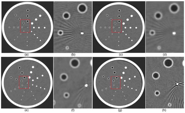
Figure 11.

Visualization of the identified inner and outer walls depicted on the CT examinations acquired on the lung phantom. (a)–(b) show the CT examinations obtained using the Siemens scanner with the B31f and B46f reconstruction kernels, respectively. (c)–(d) show the examinations obtained using the GE scanner with the bone and standard reconstruction kernels, respectively. The results of the identified tube inner and outer walls are shown in overlay in the bottom row.
Figure 12.

Comparison between our developed scheme (the top row) and the FWHM method (the bottom row) in airway wall estimation for examinations acquired on different scanners with different kernels.
The comparison of the developed scheme and the radiologist in airway wall estimation on the 50 cross sections from real lung CT examinations was shown in Figure 13. Their difference were represented by subtracting the radiologist’s result from the computerized result, ranging from −0.19 mm to 0.12 mm with a mean difference of 0.084 mm.
Figure 13.
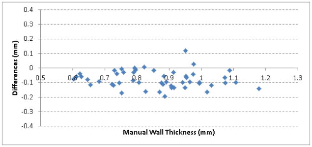
Difference of the developed scheme and the radiologist in airway wall estimation.
Figure 14 shows the results of the developed scheme in airway wall estimation when applying to the real lung CT examinations reconstructed with three different kernels. The average airway wall thicknesses estimated by the scheme for the 20 airway branches were 1.302 mm, 1.333 mm and 1.339 mm, respectively, for the examinations reconstructed with the ‘lung’, ‘bone’ and ‘standard’ kernels.
Figure 14.
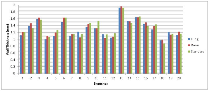
Airway wall thickness of the 20 airway branches estimated using the developed scheme in the examinations with three different kernels.
Finally, to demonstrate the performance of the scheme on real chest CT examinations, we listed in Figure 15 a number of screen-shots of the inner and outer airway walls identified using the developed scheme. These are located at various regions (e.g., trachea, bifurcation region, attachment to vessels) of an airway tree with a wide range of dimensions.
Figure 15.
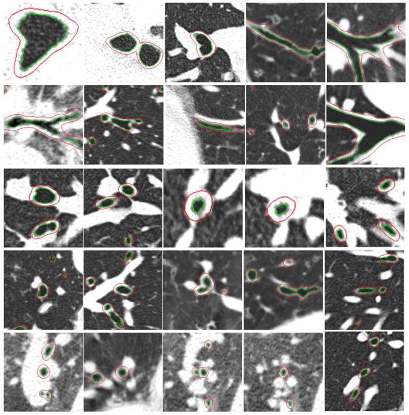
Examples demonstrating the performance of the developed scheme in identifying airway walls at different locations of an airway tree. The outer and inner airway walls are shown in overlay.
4. DISCUSSION
In this study, we described a novel computer algorithm to automatically identify airway inner/outer walls depicted in a chest CT examination by defining a novel gradient vector field and taking advantage of the relatively high contrast of airway wall. In methodology, this scheme has a number of unique characteristics. First, the airway wall identification procedure is performed on a 3D geometric surface model. Unlike most of the available relevant algorithms (Webb et al., 1984; Bankier et al., 1996; Okazawa et al., 1996; Nakano et al., 2000, 2002; Reinhardt et al., 1997) that worked in 2D/3D image space, this characteristic makes the scheme independent of airway orientations and soft tissue (e.g., adjacent vessels) attachment (Figure 15). Second, a novel external energy function is defined based on signed image gradient along a vector field instead of on the traditional magnitude of image gradient. Given the defined external and internal force fields, the model evolution will theoretically stop at the regions with the highest contrast, which typically correspond to the inner or outer airway wall. To hinder an adherence to the inner airway wall border, a previous method (Ortner et al., 2010, 2011), which used the traditional external energy function based on the magnitude of image gradient, added the balloon force during deformation. However, it is difficult to select a constant parameter for the balloon force since the image intensities and gradients may vary significant at different parts. In contrast, this scheme does not require additional balloon force or other outer forces to push the surface away from the airway border. Third, this scheme can be used to identify either airway inner wall or outer wall by simply changing the sign of the external energy function. As demonstrated by the phantom based assessment in Figures 11–12, the airway cross-sections on real lung CT examinations in Figures 13–14, and the examples in Figure 15, this scheme has a reasonable accuracy. In addition, under the help of the narrow band technique, identification of the airway inner and outer walls in a typical chest CT examination takes less than 4 minutes.
Our experiments in the phantom study showed that there are a number of factors affecting the accuracy of the airway wall estimation. First, as shown in Figure 12, there were relatively larger errors for the smaller tubes when identifying the inner airway and while for the outer walls the errors were smaller for the smaller tubes. Second, the scanners and the reconstruction kernels have impacts on the airway wall estimation as well. According to our experiments (Figure 12), the error in airway wall estimation varies from 0.05 mm to 0.35 mm, depending on airway size and scanner. Our initial experiments showed that the scheme had smaller estimation errors for the examinations obtained by the GE scanner than those obtained by the Siemens scanner. Whereas small airways play an important role in the airway obstruction observed in COPD, it is extremely important to accurately estimate the dimensions of small airway wall. However, our experiments show that this is a very challenging task. When assessing the accuracy of their method using a lung phantom, (San Jose Estépar et al., 2006) also used the examinations obtained using the Siemens scanner with the B31f and B46f reconstruction kernels. When comparing our results with theirs, we found that there was no significant difference in the estimation errors of airway wall thickness. For example, San Jose Estépar et al.’s scheme had an error of 0.3 mm for the tube with a radius of 0.9 mm in airway wall estimation for the examination with the B31f reconstruction kernel and an error of 0.2 mm for the examinations reconstructed with the B46f kernel; while our scheme has an error of 0.21 mm for a similar tube with a radius of 1.2 mm for the B46f kernel. In fact, a lung phantom is not unique for this study. Most of the available approaches airway wall identification (Reinhardt et al., 1997; Saragaglia et al., 2005; Saba et al., 2003; San Jose Estépar et al., 2006) used a lung phantom for quantitative assessment purpose. In addition, there are limitations with the tubes on the phantom, including size, orientation, and shape. (Saba et al., 2003) tried to tilt the phantom to change the orientation of the tubes and described the effects of the tilt angles in detail.
When computing the external energy function in Eq. (11), a Gaussian smoothing operation was used to improve the robustness of the scheme in the estimation of airway wall thickness. The lung phantom in Figure 9 – Figure 10 was used to determine the sigma (σ ) value. The results in Figure 16 shows the estimations errors in inner and outer airway wall when the value of the sigma is changed from 0.1 mm to 1.0 mm. As demonstrated by the experiments, the mean errors are almost the same when the sigma is smaller than 0.5 mm; otherwise, the mean errors increase obviously. Therefore, the sigma was set at 0.5 mm in this study. We are aware that determining the sigma value on the basis of the phantom data may has some limitations; however, given the “ground truth” characteristic of a lung phantom, this is actually a relatively reasonable way to determine the sigma value.
Figure 16.

Impact of the sigma on the estimation of airway (tube) wall thickness depicted on the lung phantom. The results in regard to the tubes with different sizes are denoted in different colors.
When studying the differences of the developed scheme and the radiologist in airway wall estimation (Figure 13), we found that the scheme could achieve an accuracy in reasonable agreement with a radiologist. The mean difference is only 0.084 mm. On the whole, the radiologist tends to have a larger estimation than the computerized scheme does. At the same time, our preliminary experiment on the examinations acquired on the same patients but with different construction kernels demonstrated that the reconstruction kernels had limited impact on the accuracy, because the largest average difference for the three kernels is 0.037 mm.
Finally, we are aware of the limitations of this study. First, when assessing the accuracy of the scheme on clinical chest CT examinations, we asked a radiologist to manually delineate only a very limited number of airway cross-sections on 10 CT examinations. This is largely caused by the fact that it is very time-consuming to manually process a large number of dataset. For example, (Sonka et al., 1996) reported that manual segmentation of the airway tree in a single CT examination (slice thickness in their study was 3.0 mm) required approximately seven hours of analysis. Second, when assessing the sensitivity of the scheme to the reconstruction kernels, only three CT examinations acquired on the same subject were used in this study. This is caused by the fact that it is difficult to collect CT examinations acquired on the same subjects with different reconstruction kernels. Fortunately, the characteristic that an airway tree has a large number of branches with different radii makes it possible to obtain a number of airway cross-sections. Finally, in addition to the reconstruction kernels, we are aware that there are a lot of factors that may affect the accuracy of an airway identification algorithm, e.g., partial volume effect, cone beam effect, scanners, and presence of various diseases. Obviously, in order to comprehensively investigate the sensitivities of an algorithm towards these factors, a huge effort is needed and it is beyond the scope of this study.
5. CONCLUSIONS
We described a novel computerized scheme for the identification of airway walls on CT images. A three-dimensional (3D) surface model is placed within airway regions and then evolves automatically in predefined external and internal force fields until these forces reach a state of balance. The balanced locations correspond to the boundary of the airway outer/inner wall. A preliminary study using a lung phantom and clinical chest CT examinations verified the feasibility and accuracy of the developed scheme in airway wall identification.
Highlights.
We identify airway walls by placing a surface model in a distance gradient force field.
The surface model evolves automatically until the forces reach a state of balance.
This scheme can be used to identify either airway inner wall or outer wall.
A dedicated commercial lung phantom is used for quantitative validation purpose.
The approach can achieve a reasonable performance in accuracy and efficiency.
Acknowledgments
This work was supported in part by grants HL096613, CA090440, HL084948, HL095397, 2012KTCL03-07 to the University of Pittsburgh from the National Institute of Health, the Bonnie J. Addario Lung Cancer Foundation, and the SPORE in Lung Cancer Career Development Program.
Notations in this manuscript
- A
airway lumen
- B
“narrow-band” around airway lumen with distance to A smaller than dband
- B*
a smaller “narrow-band” for distance map smoothing, B* ⊂ B
- C
regions other than A and B
- D
distance map where airway lumen A is the boundary
- D̄(Xi)
mean airway wall thickness of an airway cross-section
- E(X)
the objective (energy) function
- Eext
external energy function
- Eint
internal energy function
- Gσ
Gaussian smoothing operation with a standard deviation σ
- H
image gradient along the distance gradient field V
- I
image intensity
- Nv
the vertices number of a triangle mesh
- p
(x, y, z)T, a voxel on a CT image
- V
the distance gradient field
- X(u,s)
a geometric surface
representation of the vertices of a triangle mesh
Footnotes
Publisher's Disclaimer: This is a PDF file of an unedited manuscript that has been accepted for publication. As a service to our customers we are providing this early version of the manuscript. The manuscript will undergo copyediting, typesetting, and review of the resulting proof before it is published in its final citable form. Please note that during the production process errors may be discovered which could affect the content, and all legal disclaimers that apply to the journal pertain.
References
- Artaechevarria X, Pérez-Martín D, Ceresa M, de Biurrun G, Blanco D, Montuenga LM, van Ginneken B, Ortiz-de-Solorzano C, Muñoz-Barrutia A. Airway segmentation and analysis for the study of mouse models of lung disease using micro-CT. Phys Med Biol. 2009;54(22):7009–7024. doi: 10.1088/0031-9155/54/22/017. [DOI] [PubMed] [Google Scholar]
- Aykac D, Hoffman EA, McLennan G, Reinhardt JM. Segmentation and analysis of the human airway tree from three-dimensional X-ray CT images. IEEE Transactions on Medical Imaging. 2003;22(8):940–950. doi: 10.1109/TMI.2003.815905. [DOI] [PubMed] [Google Scholar]
- Bankier AA, Fleischmann D, Mallek R, Windisch A, Winkelbauer FW, Kontrus M, Havelec L, Herold CJ, Hübsch P. Bronchial wall thickness: Appropriate window settings for thin-section CT and radiologic-anatomic correlation. Radiology. 1996;199(3):831–836. doi: 10.1148/radiology.199.3.8638013. [DOI] [PubMed] [Google Scholar]
- Bousquet J, Jeffery PK, Busse WW, Johnson M, Vignola AM. Asthma From Bronchoconstriction to Airways Inflammation and Remodeling. Am J Respir Crit Care Med. 2000;161(5):1720–1745. doi: 10.1164/ajrccm.161.5.9903102. [DOI] [PubMed] [Google Scholar]
- Berger P, Perot V, Desbarats P, Tunon-de-Lara JM, Marthan R, Laurent F. Airway wall thickness in cigarette smokers: Quantitative thin-section CT assessment. Radiology. 2005;235(3):1055–1064. doi: 10.1148/radiol.2353040121. [DOI] [PubMed] [Google Scholar]
- Cohen D. On active contour models and balloons. CVGIP: Image Understand. 1991;53:211–218. [Google Scholar]
- Cornea ND, Silver D, Yuan X, Balasubramanian R. Computing hierarchical curve-skeletons of 3-D objects. Visual Comput. 2005;21(11):945–955. [Google Scholar]
- Graham MW, Gibbs JD, Cornish DC, Higgins WE. Robust 3-D Airway Tree Segmentation for Image-Guided Peripheral Bronchoscopy. IEEE Transactions on Medical Imaging. 2010;29(4):982–997. doi: 10.1109/TMI.2009.2035813. [DOI] [PubMed] [Google Scholar]
- Kass M, Witkin A, Terzopoulos D. Snakes: Active contour models. International Journal of Computer Vision. 1987;1:321–331. [Google Scholar]
- Lorensen WE, Cline HE. Marching Cubes: A high resolution 3D surface construction algorithm. SIGGRAPH Computer Graphics. 1987;21(4):163–169. [Google Scholar]
- Montaudon M, Berger P, de Dietrich G, Braquelaire A, Marthan R, Tunon-de-Lara JM, Laurent F. Assessment of Airways with Three-dimensional Quantitative Thin-Section CT: In Vitro and in Vivo Validation1. Radiology. 2007;242(2):563–572. doi: 10.1148/radiol.2422060029. [DOI] [PubMed] [Google Scholar]
- Nakano Y, Muro S, Sakai H, Hirai T, Chin K, Tsukino M, Nishimura K, Itoh H, Paré PD, Hogg JC, Mishima M. Computed tomographic measurements of airway dimensions and emphysema in smokers - Correlation with lung function. American Journal of Respiratory and Critical Care Medicine. 2000;162:1102–1108. doi: 10.1164/ajrccm.162.3.9907120. [DOI] [PubMed] [Google Scholar]
- Nakano Y, Whittall KP, Kalloger SE, Coxson HO, Flint J, Pare PD. Development and validation of human airway analysis algorithm using multidetector row CT. SPIE Medical Imaging. 2002:460–469. [Google Scholar]
- Okazawa M, Muller N, Mcnamara AE, Child S, Verbrgt L, Pare PD. Human airway narrowing measured using high resolution computed tomography. American Journal of Respiratory and Critical Care Medicine. 1996;154(5):1557–1562. doi: 10.1164/ajrccm.154.5.8912780. [DOI] [PubMed] [Google Scholar]
- Ortner M, Fetita C, Brillet PY, Prêteux F, Grenier P. 3D Vector Flow Guided Segmentation of Airway Wall in MSCT. the 6th international conference on Advances in visual computing; 2010. pp. 302–311. [Google Scholar]
- Ortner M, Fetita C, Brillet PY, Prêteux F, Grenier P. Surface modeling and segmentation of the 3D airway wall in MSCT. Proc. SPIE Conference on Medical Imaging; 2011. p. 79640O-79640O-12. [Google Scholar]
- Park W, Hoffman EA, Sonka M. Segmentation of intrathoracic airway trees: A fuzzy logic approach. IEEE Transactions on Medical Imaging. 1998;17:489–497. doi: 10.1109/42.730394. [DOI] [PubMed] [Google Scholar]
- Pu J, Fuhrman C, Good WF, Sciurba FC, Gur D. A Differential Geometric Approach to Automated Segmentation of Human Airway Tree. IEEE Transactions on Medical Imaging. 2011;30(2):266–278. doi: 10.1109/TMI.2010.2076300. [DOI] [PMC free article] [PubMed] [Google Scholar]
- Pu J, Leader JK, Meng X, Whiting B, Wilson D, Gur D, Sciurba F, Reilly JJ, Bigbee WB, Siegfried J. Academic Radiology. 2012. Three-dimensional Airway Tree Architecture and Pulmonary Function. in press. [DOI] [PMC free article] [PubMed] [Google Scholar]
- Reinhardt JM, D’Souza ND, Hoffman EA. Accurate measurement of intrathoracic airways. IEEE Transactions on Medical Imaging. 1997;16(6):820–827. doi: 10.1109/42.650878. [DOI] [PubMed] [Google Scholar]
- Saba OI, Hoffman EA, Reinhardt JM. Maximizing quantitative accuracy of lung airway lumen and wall measures obtained from X-ray CT imaging. Journal of Applied Physiology. 2003;95(3):1063–1075. doi: 10.1152/japplphysiol.00962.2002. [DOI] [PubMed] [Google Scholar]
- San Jose Estépar R, Washko GG, Silverman Ek, Reilly JJ, Westin CF. Accurate airway wall estimation using phase congruency. Medical Image Computing and Computer-Assisted Intervention - Miccai; 2006; 2006. pp. 125–134. [DOI] [PubMed] [Google Scholar]
- Saragaglia A, Fetita C, Brillet PY, Grenier PA. Accurate 3D quantification of the bronchial parameters in MDCT. SPIE Medical Imaging. 2005:323–334. [Google Scholar]
- Sonka M, Park W, Hoffman EA. Rule-based detection of intrathoracic airway trees. IEEE Transactions on Medical Imaging. 1996;15(3):314–326. doi: 10.1109/42.500140. [DOI] [PubMed] [Google Scholar]
- Tschirren J, Hoffman EA, McLennan G, Sonka M. Intrathoracic airway trees: Segmentation and airway morphology analysis from low-dose CT scans. IEEE Transactions on Medical Imaging. 2005;24(12):1529–1539. doi: 10.1109/TMI.2005.857654. [DOI] [PMC free article] [PubMed] [Google Scholar]
- van Ginneken B, Baggerman W, van Rikxoort EM. Robust Segmentation and Anatomical Labeling of The Airway Tree from Thoracic CT Scans. MICCAI. 2008:219–226. doi: 10.1007/978-3-540-85988-8_27. [DOI] [PubMed] [Google Scholar]
- Webb WR, Gamsu G, Wall SD, Cann CE, Proctor E. Ct of a Bronchial Phantom - Factors Affecting Appearance and Size Measurements. Investigative Radiology. 1984;19(5):394–398. doi: 10.1097/00004424-198409000-00011. [DOI] [PubMed] [Google Scholar]
- Weinheimer O, Achenbach T, Bletz C, Duber C, Kauczor HU, Heussel CP. About objective 3-d analysis of airway geometry in computerized tomography. IEEE Transactions on Medical Imaging. 2008;27(1):64–74. doi: 10.1109/TMI.2007.902798. [DOI] [PubMed] [Google Scholar]
- Xu C, Prince JL. Generalized gradient vector flow external forces for active contours. Signal Processing. 1998;71(2):131–139. [Google Scholar]