Wavelet Transform-Based De-Noising for Two-Photon Imaging of Synaptic Ca²⁺ Transients

Abstract

Postsynaptic Ca²⁺ transients triggered by neurotransmission at excitatory synapses are a key signaling step for the induction of synaptic plasticity and are typically recorded in tissue slices using two-photon fluorescence imaging with Ca²⁺-sensitive dyes. The signals generated are small with very low peak signal/noise ratios (pSNRs) that make detailed analysis problematic. Here, we implement a wavelet-based de-noising algorithm (PURE-LET) to enhance signal/noise ratio for Ca²⁺ fluorescence transients evoked by single synaptic events under physiological conditions. Using simulated Ca²⁺ transients with defined noise levels, we analyzed the ability of the PURE-LET algorithm to retrieve the underlying signal. Fitting single Ca²⁺ transients with an exponential rise and decay model revealed a distortion of τ_rise but improved accuracy and reliability of τ_decay and peak amplitude after PURE-LET de-noising compared to raw signals. The PURE-LET de-noising algorithm also provided a ∼30-dB gain in pSNR compared to ∼16-dB pSNR gain after an optimized binomial filter. The higher pSNR provided by PURE-LET de-noising increased discrimination accuracy between successes and failures of synaptic transmission as measured by the occurrence of synaptic Ca²⁺ transients by ∼20% relative to an optimized binomial filter. Furthermore, in comparison to binomial filter, no optimization of PURE-LET de-noising was required for reducing arbitrary bias. In conclusion, the de-noising of fluorescent Ca²⁺ transients using PURE-LET enhances detection and characterization of Ca²⁺ responses at central excitatory synapses.

Introduction

Single transmission events at excitatory synapses in the central nervous system elicit fast, short-lived rises in postsynaptic cytosolic [Ca²⁺] (Ca²⁺ transients). These transients encode intracellular signals with physiological consequences ranging from the modulation of synaptic currents to long-term changes in synaptic efficacy (1,2). Ca²⁺ transients are readily detected with intracellular Ca²⁺-sensitive dyes in minute (1–2 μm) structures such as dendritic spines, using two-photon laser-scanning fluorescence microscopy (TPLSM) (3–5). This technique offers excellent optical penetration and diffraction-limited excitation volume in structures embedded deep within brain tissue. In combination with electrophysiology, TPLSM allows the optical recording of locally elicited excitatory postsynaptic Ca²⁺ transients (EPSCaTs) at single spines, simultaneously with the synaptic electrical response recorded at the soma (6). These techniques may be employed to determine how spine EPSCaTs encode specific patterns of synaptic activity that trigger or modulate synaptic plasticity (7–11). Due to technical constraints, the available information concerning EPSCaT time-course is limited, despite its importance (12,13).

Accurate measurements of EPSCaT amplitude and time-course require high spatial and temporal resolution, and rely on high gain photomultiplier tubes (PMTs) to detect small, photon-noise-limited, fluorescence signals (14,15). Due to high sampling rate and reduced fluorophore availability given the small cellular compartments where they occur, EPSCaTs tend to be low-photon-count events. Consequently, EPSCaT analysis is hampered by measurement noise seen as the uncertainty in pixel values, which report the underlying fluorescence intensity. To resolve the small signals, experiments may be biased toward stronger synapses, and the risk of photodamage is increased as more repetitions are required for an average response. Several methods have therefore been developed to enhance the peak signal/noise ratio (pSNR) of the recorded fluorescence transients.

Apart from the use of low-noise expensive custom-made hardware (3), the choice of fluorescent Ca²⁺ indicators can improve the quality of the Ca²⁺ signals, but each has drawbacks (16,17). High-affinity dyes produce less noisy signals, but due to added buffer capacity can underestimate the change in [Ca²⁺], and can saturate during stimulus trains. Medium-affinity dyes have a linear range better suited for trains of pre- and postsynaptic stimuli, but give off dimmer signals. At glutamatergic synapses, Ca²⁺ responses can be enhanced by removing extracellular Mg²⁺ or depolarizing the postsynaptic cell to relieve the constitutive Mg²⁺ block of NMDA receptors (18–20). However, depolarization or removal of Mg²⁺ is nonphysiological and therefore limited to providing an indirect optical measure of neurotransmitter release. Alternatively, Ca²⁺ signals with good pSNR from individual spines have been obtained using two-photon photolysis of caged neurotransmitters (21,22), with the caveat that the glutamate released may not accurately replicate the time course of endogenous neurotransmitter in the synaptic cleft and may activate more extrasynaptic receptors than synaptic release (23).

An alternative approach to improve the effective pSNR for EPSCaTs is to apply a signal-processing algorithm that can recover EPSCaTs from noisy recordings obtained with commonly available hardware. Typical approaches use low-pass or binomial filtering with a moving average window of arbitrary size (2–33 samples), time-averaging of an arbitrary number of (successful) trials, or a combination of these (7,11,18,24–26). Classical low-pass filtering cleans up the signal by removing the high-frequency components (thought to concentrate the noise) and therefore tends to oversmooth the signal (27), thus introducing measurement errors for time constants and peak amplitudes. Because of the trade-off between improving the pSNR and the accuracy of inferred signal parameters, finding an optimal low-pass filter type and size has remained elusive. Time-averaging assumes a stationary synaptic response to repeated identical stimuli, contrary to some observations (26), and, because of increased exposure to excitation light and consequent photobleaching and phototoxicity, it prevents complex experiments from being performed on the same synapse (28).

A distinct de-noising technique is based on the wavelet transform, a decomposition of a signal in terms of localized basis functions, or wavelets. Mathematically analogous to the Fourier transform, which realizes a frequency analysis of the signal as a whole, the wavelet transform creates a multiresolution representation of the signal (29). One immediate consequence is that noise is decorrelated from local features of the signal, and can be removed with minimal alterations to the underlying signal (30). In this paradigm, the noise is considered a stationary random process whereas the underlying signal is treated either as deterministic or stochastic. Wavelet transform-based de-noising works in three fundamental steps:

• Step 1. The signal is transformed in the wavelet domain to generate a set of wavelet coefficients representing local signal features at a range of resolutions, and a coarse (smooth) approximation of the signal.

• Step 2. The result from Step 1 is passed through a wavelet shrinkage and thresholding algorithm (31) adapted to the statistical properties of the noise.

• Step 3. The processed coefficients are transformed back into the signal domain, to obtain a de-noised estimate of the signal.

In fluorescence microscopy imaging, measurement noise arises primarily from the Poisson distribution of the photon counts arriving at the photodetector device and the uncertainties in the photoelectron emission, compounded by thermal fluctuations that amount to added white Gaussian noise (AWGN) (32–34). Data samples are viewed as realizations of random variables with Poisson distribution having the mean and variance equal to the intensity of the underlying signal, and thus, the level of noise is intrinsically dependent on signal intensity. Previously, applications of wavelet de-noising to Ca²⁺ fluorescence imaging assumed a Gaussian approximation of the measurement noise (35). However, this approximation breaks down for low-photon-count imaging commonly encountered for spine EPSCaTs. A group of wavelet-based techniques was developed specifically for time-varying signals with a mixture of Poisson and Gaussian noise (36). Here, we have applied a state-of-the-art wavelet-based de-noising algorithm designed for de-noising images corrupted by mixed Poissonian and Gaussian noise (Poisson unbiased risk estimate-linear expansion of thresholds, PURE-LET) (33), to recover EPSCaTs from TPLSM recordings made from single dendritic spines in CA1 neurons in acute hippocampal slices.

Materials and Methods

Slice preparation

Acute hippocampal slices were prepared with 200–250 g male Wistar rats after inhalation of a lethal dose of Isoflurane anesthetic. Brains were dissected in ice-cold aCSF (119 mM NaCl, 2.5 mM KCl, 1 mM NaH₂PO₄, 26.2 mM NaHCO₃, 10 mM glucose, 2.5 mM CaCl₂, and 1.3 mM MgCl₂, 300 mOsm) equilibrated with 95% CO₂ and 5% O₂ and horizontal hippocampal slices (400-μm thick) were cut with a VT1200 vibratome (Leica, Wetzlar, Germany). Slices were incubated in aCSF at 36°C for 30 min, then at room temperature before use. The procedures were carried out in accordance with Home Office guidelines as directed by the Home Office Licensing Team at the University of Bristol.

Electrophysiology and two-photon Ca²⁺ imaging

Whole-cell recordings were made from CA1 pyramidal cells visualized with infrared differential interference contrast optics on a model No. BX-51 microscope (Olympus UK, Southend-on-Sea, UK) in a recording chamber perfused with aCSF (35°C) containing 50 μM picrotoxin. Patch electrodes (5–6 MΩ) were pulled from borosilicate filamented glass capillaries (Harvard Apparatus, Edenbridge, UK) and filled with intracellular solution containing: 117 mM KMeSO₃, 8 mM NaCl, 1 mM MgCl₂ 10 mM HEPES, 4 mM MgATP, 0.3 mM Na₂GTP, and 0.2 mM EGTA, buffered to pH 7.2, 280 mOsm. The intracellular solution was supplemented with Ca²⁺ fluorescent indicator (Fluo-5F, 300 μM) and a reference fluorescent dye (Alexa Fluor 594, 30 μM) from stock solutions (Invitrogen, Paisley, UK).

For synaptic stimulation, an aCSF-filled extracellular glass electrode (6–7 MΩ) was placed in the stratum radiatum, ∼100–200 μm from the pyramidal cell layer. Whole-cell patch-clamp configuration was established under voltage-clamp (−70 mV), then cells were switched to current clamp and dye-loaded by injecting 100–150 pA inward current for 10–15 min using an AxoPatch 200B amplifier (Molecular Devices, Wokingham, UK) before imaging. Resting membrane potential was continually monitored and cells with resting membrane potentials above −60 mV or drifting by >10 mV were discarded. Membrane potentials were not corrected for the liquid junction potential, which was calculated to be 9 mV. Signals were filtered at 5 kHz and digitized at 10 kHz via a CED Micro 1401 MKII, using Signal 2 software (Cambridge Electronic Design, Cambridge, UK).

Alexa Fluor 594 (Alexa) and Fluo-5F fluorescence was visualized via a LUMPlanFl 60× W/IR (0.9 NA) water immersion objective (Olympus), using a Radiance 2100 MP two-photon system (Bio-Rad, Berkeley, CA) equipped with a Mai Tai BB Ti:Sapphire laser (Newport Spectra-Physics, Didcot, UK), tuned to 810 nm.

After an initial 10–15 min dye-loading, spines on secondary dendrites of the cell being patched were initially imaged in raster scanning mode (∼4.5 frames/s) to allow for the placement of the stimulating electrode tip at ∼50 μm distance. Synaptic responses were elicited every 10 s by delivering 1 ms electrical pulses from a DS2A-mkII Isolated Constant Voltage Stimulator (Digitimer, Welwyn Garden City, UK), via the extracellular electrode. The stimulus amplitude was adjusted to yield subthreshold excitatory postsynaptic potentials. Optically responsive spines (displaying stimulus-triggered EPSCaTs) were iteratively searched by imaging individual spines in line-scanning mode (1200 lines/s) while delivering pairs of stimuli (25-ms apart, to increase the release probability). Stimulus delivery was synchronized to 0.1 s after the start of each line-scan series. Once a responsive spine was identified, subsequent Ca²⁺ transient recordings were performed at 0.2 Hz in line-scanning mode. Any required adjustments to the position of the electrode and image focus were made by briefly switching to raster-scanning mode between successive Ca²⁺ transient recordings.

Images (8-bit quantization) were acquired with LaserSharp2000 v.6.0 software (Carl Zeiss, Welwyn Garden City, UK) and analyzed offline using software written in the software MATLAB (The MathWorks, Cambridge, UK). Software gain settings were, respectively: 20 for the Alexa channel, and 30 for the Fluo-5F channel. The projection image in Fig. 1 a was generated with the software ImageJ (National Institutes of Health, Bethesda, MD) (37). Fluorescence intensities are expressed as pixel gray level in arbitrary units (a.u.).

Figure 1.

Spine EPSCaT recordings from a CA1 pyramidal neuron in a hippocampal slice. (a) (Left) Montage of maximum intensity projections of two TPLSM z-stacks of a CA1 pyramidal neuron in a hippocampal slice loaded with the fluorescent Ca²⁺ dye Fluo-5F and Alexa Fluor 594 (Alexa). (Open rectangle, zoomed in top right) Location of the scanning line across a spine head. (Bottom right) Primary data consisting of line-scan XT images with Fluo-5F and Alexa channels (0.08 μm/pixel × 1200 lines/s, 1 s, temporal axis vertical) synchronized with a single stimulus (arrowhead) delivered via the extracellular electrode. The spine region of interest is labeled beneath the Alexa line-scan image. (b) (Top to bottom) Fluorescence traces calculated by summating line-scan images row-wise within the spine region of interest, the calculated EPSCaT trace, and associated EPSP. (Vertical scale bars) 100 a.u. (Fluo-5F and Alexa), 10% (EPSCaT), and 5 mV (EPSP). (c) Time-average for images (left) and traces (right) of 30 consecutive sweeps through the spine imaged in panel a. Average Fluo-5F and calculated EPSCaT traces are fitted with a double exponential function (Eq. 2). Vertical scale bars: 50 a.u. (Fluo-5F) and 50% (EPSCaT). Horizontal scale bars in panels b and c: 0.1 s.

Analysis of Ca²⁺ transient data and the two-dimensional EPSCaT model

One-dimensional spine Ca²⁺ transients (one-dimensional EPSCaTs) were calculated from two-channel fluorescence data according to Eq. 1 (5),

$$y\left(t\right)=\frac{\Delta F}{A}=\frac{F-F_0}{A},$$ (1)

where A and F are the instantaneous fluorescence intensities in the Alexa and Fluo-5F channels, respectively, and F₀ is the mean resting Fluo-5F fluorescence intensity. Five kinetic parameters for the one-dimensional EPSCaTs: scale (a), offset (b), the rise time constant (τ_rise), the decay time constant (τ_decay), and the onset of the transient (t₀) were determined by fitting with the exponential rise and decay function in Eq. 2:

$$y\left(t\right)=a\times \left(1-e^{\raisebox{1ex}{$-\left(t-t_0\right)$}\!\left/ \!\raisebox{-1ex}{${\tau }_{\text{rise}}$}\right.}\right)\times e^{\raisebox{1ex}{$-\left(t-t_0\right)$}\!\left/ \!\raisebox{-1ex}{${\tau }_{\text{decay}}$}\right.}+b.$$ (2)

Synthetic two-dimensional spine Ca²⁺ transients (two-dimensional EPSCaTs) were generated by combining the one-dimensional EPSCaT model in Eq. 2 with a spatial one-dimensional Gaussian spine profile model (see Eq. S1 and Fig. S1 in the Supporting Material). A more detailed description of this method is given in the Supporting Material.

Measurement noise model

Measurement noise in the two-dimensional EPSCaTs was simulated according to the multiplicative and additive noise model (Eq. 3) (33),

$$\mathbf{y}=\mathbf{z}+\mathbf{b},\text{with:}\mathbf{z}\approx \alpha P\left(\mathbf{x}\right),\text{and}\mathbf{b}\approx N\left(\mathbf{\delta },{\sigma }^2\mathbf{I}\right),$$ (3)

where the pixel intensities in the fluorescence image (y) result from the summation of a scaled-Poisson process (z) parameterized on the fluorescence intensity (x) and a stationary, additive normally-distributed random noise b with mean δ and variance σ². The time- and space-varying fluorescence intensity signal x is considered deterministic. The noise parameters α, σ², and δ were determined from image sample mean and variance estimated on 8 × 8 pixel image windows according to Luisier et al. (33) and Boulanger et al. (38) (see Fig. S2 b). A justification of the noise model used, together with algorithmic details, is given in the Supporting Material.

Algorithm implementation

The PURE-LET de-noising algorithm was implemented using nondecimated two-dimensional wavelet transform in the Haar wavelet basis, according to Luisier et al. (33). Filtering with moving average window or binomial filters was implemented using the MATLAB Image Processing Toolbox. The binomial filters were generated as the outer vector product of one-dimensional finite impulse response kernels according to Eq. 4 (25),

$$h\left[k\right]=\left(\begin{array}{c}2p\\ p+k\end{array}\right)\times \frac{1}{4^p},$$ (4)

where h is a filter kernel with 2p + 1 coefficients, h[k] is the k^th coefficient, p is the order of the filter, and $\left(\begin{array}{c}a\\ b\end{array}\right)$ denotes the binomial coefficient. Curve-fitting was done using MATLAB’s constrained nonlinear least-square optimization routine lsqnonlin.

The empirical density estimates seen later in Figs. 4 and 5 were obtained using a fast kernel density estimator (39). All procedures were written in MATLAB.

Figure 4.

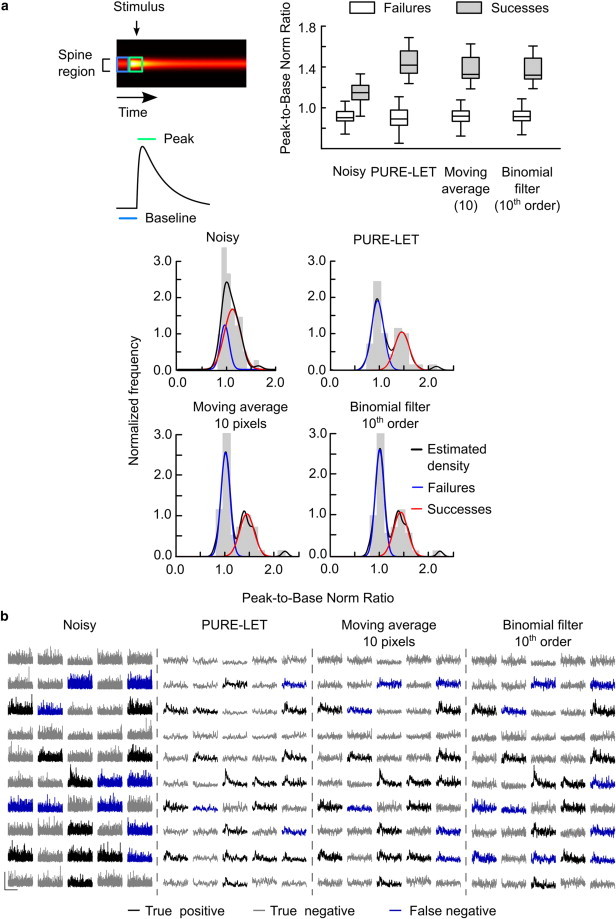
Discrimination of failures in simulated EPSCaTs. (a) (Top left) Schematic of the discrimination criterion, calculated from peak and baseline regions defined on two-dimensional primary Ca²⁺ fluorescence signal (one-dimensional projection is shown below). (Top right) Peak/base norm ratio (median, 25th and 75th quartiles, and range) for the failures and successes in noisy, de-noised, and filtered data from 50 simulated trials. (Bottom) Probability distribution of the peak/base norm ratio for the noisy, de-noised, and filtered data sets from 50 trials, with the empirical density estimate (density) and Gaussian fits for the two populations of failures and successes. (b) Classification outcome on the simulated noisy traces and after de-noising or filtering. Scale bars, vertical: 200 a.u. (noisy data), 100 a.u. (de-noised and filtered data); horizontal: 0.5 s.

Figure 5.

Discrimination of failures in experimental data. (a) Distributions of the peak/base norm ratio calculated for 60 sweeps of experimental data before and after de-noising, or filtering. The density estimates together with their fits with three Gaussians (failures plus two success groups) are also shown. (b) Examples of traces before and after de-noising or filtering. Scale bars: 10% ΔF/A (vertical), 0.5 s (horizontal).

Results

To record EPSCaTs we loaded CA1 pyramidal neurons with a calcium indicator (Fluo-5F) and a reference dye (Alexa Fluor 594, Alexa) through a patch electrode at the soma (Fig. 1 a). Because Fluo-5F has low background fluorescence, the reference dye is essential to visualize the dendritic spines and to calculate the relative change in Ca²⁺ fluorescence. Spinous EPSCaTs are then elicited by locally stimulating axonal fibers that synapse onto the patched cell, by delivering short electrical pulses through an extracellular electrode near to the neuron’s apical dendrites. Fluorescence in both Fluo-5F and Alexa channels is then recorded by successive line-scans across the spine head, to generate a two-dimensional time-space (XT) image of fluorescence intensities (primary data, Fig. 1 a). The EPSCaT signal represents the relative change in Ca²⁺ fluorescence (Fig. 1 b, EPSCaT trace) calculated from a one-dimensional time-series of fluorescence intensities obtained by summating primary data row-wise over the spine region of interest (Fig. 1 b, Fluo-5F and Alexa traces). Stimulus-induced transients, when they occur, are time-locked with the simultaneously recorded excitatory postsynaptic potential (EPSP) elicited by the stimulus.

Simulation of EPSCaTs

To assess the performance of the PURE-LET de-noising algorithm, we generated synthetic two-dimensional EPSCaTs with defined noise levels. According to Eq. 1, the fluorescence intensity in the Alexa channel merely helps compensate for intensity fluctuations independent of the Ca²⁺ transient. Therefore, we concentrated on simulating the Fluo-5F line-scanning XT images. We note, however, that in real life both Fluo-5F and Alexa channels are subjected equally to measurement noise and hence they should both be processed before calculating the EPSCaT signal. Thus we simulated two-dimensional Fluo-5F fluorescence to replicate recorded Ca²⁺ fluorescence primary data such as that depicted in Fig. 1.

To obtain a realistic set of EPSCaT parameters for our simulations, we fitted one-dimensional Fluo-5F fluorescence time-course data obtained from a series of 30 EPSCaTs (Materials and Methods, Fig. 1 c and see Fig. S1). The series was previously recorded ex vivo from a CA1 hippocampal pyramidal neuron (Fig. 1 a). We then used the fitted values of the parameters (scale: 76.62 a.u, and offset: 43.33 a.u.), and of the rise and decay time constants (3.7 ms and 112.6 ms, respectively) to simulate an idealized (or clean) one-dimensional EPSCaT in the temporal axis. Note that the values of these parameters are characteristic of the average Ca²⁺ response of the spine to synaptic stimulation.

In most two-photon laser-scanning systems where fluorescence is detected using photomultiplier devices (PMT), measurement noise arises from a combination of multiplicative and additive processes associated with the stochastic nature of the incident photon flux and the photodetection process in the PMT (Materials and Methods, Fig. 2 a, and see the Supporting Material). We approximated measurement noise by a scaled Poisson process summated with AWGN (Eq. 3) (33). To verify the general noise model in Eq. 3 for low photon-counts, we first obtained experimental background fluorescence data in the Fluo-5F channel.

Figure 2.

Simulations of noisy two-dimensional EPSCaT data. (a) Depiction of signal and noise amplification across dynodes D₁ to D_n in a photomultiplier tube. In high-gain PMTs the output is dominated by the distribution P (λ) of the secondary electrons after the first dynode. Analog to digital converter (ADC). (b) Examples of simulated two-dimensional Fluo-5F fluorescence for an idealized Ca²⁺ transient (Model), a noisy realization (Simulated), and the experimental data reproduced in the simulation. (Bottom traces) Simulated and experimental fluorescence intensity profiles with fitted exponential rise and decay. Calibration bar values are in a.u. (c) Peak SNR as a function of simulated photon efficiency given the same underlying signal (left) and as a function of signal amplitude for the same photon efficiency (middle). (Right) Peak SNR (median, 25th and 75th quartiles, and range) for the experimental data set (Exp.) of 30 sweeps used in Fig. 1.

The data set (256 × 1200 pixels corresponding to 20.43 μm × 1 s) was recorded by line-scan imaging in a microscope field devoid of fluorophore (see Fig. S2), using the same gain and offset software settings, sampling rates, and quantization levels as for our experimental data in Fig. 1. The scaling factor for the Poisson noise component (α: 10.7), the variance (σ²: 0.8), and mean (δ: 0) of the AWGN were determined as described in Materials and Methods. We then used these values to synthesize a noisy image by using Eq. 3 with the fluorescence intensity x set to the sample mean of the nonzero pixels in the recorded background data (3.9 a.u.). The distribution of pixel intensities in the resulting synthetic noisy background data and the measured values for α-, σ²-, and δ-parameters agreed well with those for the experimental background data (see Fig. S2).

To synthesize two-dimensional EPSCaTs containing noise levels similar to those in experimental data, we first estimated the overall level of noise associated with experimental EPSCaTs where noise variance is linked to the underlying signal intensity. To this end, we used the pSNR, expressed in decibel (dB) and defined in Eq. 5, where y_max is the maximum value in the clean signal, and MSE is the mean-squared error between the clean signal y and its noisy realization. This parameter is a commonly used objective measure of noise level in fluorescence imaging (33,38),

$$pSNR=10{\text{log}}_{10}\left(\frac{{\left(y_{\max }\right)}^2}{MSE}\right).$$ (5)

Because the underlying clean signal from experimental data was unavailable to estimate the pSNR, we synthesized clean two-dimensional EPSCaTs using fitted parameters for individual recorded sweeps and used them as the clean signal in Eq. 5. The range of pSNR in experimentally recorded data varied broadly (Fig. 2 c), consistent with a large variability in the amplitude of the peak Ca²⁺ transients (e.g., see later in Fig. 5).

We initially synthesized a two-dimensional EPSCaT for which the scale parameter (a) of Eq. 2 was set to a value commonly found by fitting our experimental data directly (50 a.u.). Note that this peak value actually represents the summation of data from 12 pixels corresponding to the spine region of interest modeled as described in the Supporting Material. We then generated a set of noisy realizations of this data according to Eq. 3 (see Materials and Methods). The PMT quantum efficiency is difficult to measure directly. However, the probability π of the binomial selection process used in our noise modeling (see Materials and Methods and the Supporting Material) can be considered to reflect the overall photon efficiency of the TPLSM system due to some of the emitted fluorescence photons being lost on the way to the photodetector (40).

To obtain a realistic estimate for this probability, we first varied the simulated photon efficiency and compared the pSNR of the outcome to that of our experimental data (Fig. 2 c). At photon efficiencies of 0.3, 0.35, and 0.4 the pSNR was, respectively, 7.8 dB, 8.5 dB, and 9.2 dB. These values were close to the experimental data pSNR (median ± interquartile range, IQR: 8.7 ± 4.1 dB). Next, we simulated noisy two-dimensional EPSCaTs by fixing the simulated photon efficiency to 0.3, corresponding to the contemporary estimates for the best PMTs (32) and allowing the scale parameter (a) of Eq. 2 to vary across a range of values typical of our recorded data. The pSNR values agreed well with those estimated from experimental data (Fig. 2 c).

Thus, by applying Eq. 3 with a fixed PMT efficiency of 0.3, we produced noisy data similar to that seen in experimental two-dimensional EPSCaTs, but with the benefit of a defined underlying noise-free signal (Fig. 2, b and c).

Wavelet de-noising of simulated data

To determine the performance of PURE-LET de-noising on our data, we processed the noisy data generated from simulated two-dimensional EPSCaTs (photon efficiency, 0.3; signal/scale, 50 a.u) by applying the algorithm of Luisier et al. (33). We compared the pSNR of the output to that of the classical filtering methods with a range of moving average and binomial (25) filter sizes commonly used to enhance the pSNR in recorded EPSCaTs (3,6,7,11,18,24,26,41) (Fig. 3 a). The results for 50 simulations are shown in Fig. 3 b. The pSNR for unprocessed (noisy) data was 7.9 ± 0.07 dB (mean ± standard deviation, SD). PURE-LET de-noising yielded a pSNR of 37.76 dB ± 0.28 dB corresponding to ∼30 dB gain in pSNR. In contrast, pSNR after classical filtering varied nonlinearly with the size of the filter kernel, with the best gain in pSNR being roughly half of that of PURE-LET (maximum pSNR was 22.3 ± 0.22 dB, and 24.2 ± 0.28 dB, respectively, for a moving average filter of 10 × 10 pixels and 10th order binomial filter corresponding to 21 × 21 pixels).

Figure 3.

Performance of PURE-LET de-noising and classical filtering algorithms on EPSCaT parameter recovery from simulated noisy data. (a) The outcome of processing the simulated noisy two-dimensional EPSCaT in Fig. 2 with PURE-LET, moving average, and binomial filtering. (Top) Processed two-dimensional signals. (Bottom) The one-dimensional EPSCaT traces with overlaid fitted curves. Calibration bar values are in a.u. (b) Five measures of performance (pSNR, R² goodness-of-fit, and signal parameters) and the global figure-of-merit for the recovery of EPSCaT parameters from unprocessed (Noisy) and processed data. Values are mean ± standard deviation from 50 simulations. Latent signal: the underlying signal parameters values used for the simulations.

An important aim in de-noising EPSCaT data is to render them suitable for further analysis, e.g., by fitting the Ca²⁺ transient model given in Eq. 2. Therefore, we determined the ability of PURE-LET and classical filtering algorithms to recover the original EPSCaT parameters by fitting the model in Eq. 2 to the one-dimensional EPSCaT obtained from the de-noised or filtered data (see Materials and Methods). To this end, we compared the fitted values of the amplitude, τ_rise and τ_decay with the reference values generated by fitting the one-dimensional trace derived from the clean two-dimensional EPSCaT, and used the degrees of freedom-adjusted coefficient of determination R² (42) as a measure of the reliability of the fit (Fig. 3 b). Table 1 shows that PURE-LET de-noising resulted in highly reliable model fits, with statistically not significant bias in amplitude and τ_decay but a significant bias in τ_rise. By comparison, moving average or binomial filtering approached the R² values for PURE-LET de-noised data as the size of the filter kernel increased, for the price of larger bias in individual EPSCaT parameters. Filters with size <10 did not distort τ_rise as much as PURE-LET de-noising but also had limited reliability (low R² values).

Table 1.

PURE-LET and classical filtering algorithms performance in latent signal parameter estimation and signal/noise ratio enhancement

Algorithm (filter order/size)	Parameter bias % (mean ± SD and p-values)			R2 Goodness of fit	pSNR (dB)	Global FOM
	Amplitude	τdecay	τrise
PURE-LET	−0.18 ± 3.79, 0.74	0.32 ± 8.63, 0.8	45.8 ± 67.67, < 0.01	0.97 ± 0.01	37.76 ± 0.28	0.9 ± 0.05
Binomial filter 2	0.09 ± 3.83, 0.86	−0.02 ± 8.07, 0.99	4.04 ± 53.39, 0.59	0.76 ± 0.01	19.19 ± 0.11	0.75 ± 0.04
Binomial filter 10	−5.66 ± 3.22, < 0.01	−0.4 ± 8.03, 0.72	20.26 ± 51.14, 0.01	0.88 ± 0.01	24.19 ± 0.29	0.81 ± 0.04
Binomial filter 25	−14.15 ± 2.8, < 0.01	−0.79 ± 8.03, 0.49	42.85 ± 53, < 0.01	0.92 ± 0.01	21.55 ± 0.24	0.77 ± 0.04
Binomial filter 100	−38.03 ± 1.87, < 0.01	−1.79 ± 8.25, 0.13	123.5 ± 60.46, < 0.01	0.96 ± 0.01	14.72 ± 0.08	0.62 ± 0.03
Moving average 2	2.21 ± 4.15, < 0.01	−0.04 ± 8.01, 0.97	2.04 ± 56.71, 0.8	0.62 ± 0.02	13.8 ± 0.07	0.67 ± 0.04
Moving average 10	−9.48 ± 3.04, < 0.01	−0.59 ± 8.02, 0.61	31.79 ± 52.29, < 0.01	0.9 ± 0.01	22.32 ± 0.23	0.79 ± 0.04
Moving average 30	−53.91 ± 1.4, < 0.01	−2.45 ± 8.43, 0.05	195.34 ± 65.15, < 0.01	0.97 ± 0.01	11.82 ± 0.04	0.55 ± 0.02
Unprocessed	1.86 ± 4.37, < 0.01	0.18 ± 8.07, 0.87	−0.19 ± 55.82, 0.98	0.44 ± 0.02	7.91 ± 0.07	0.58 ± 0.04

Table shows the fitted parameter bias expressed as a fraction of the reference values, together with R², pSNR and FOM. Also shown are the p-values for a two-tailed t-test of the null hypothesis that the bias values are normally distributed with zero mean. For clarity, values are only listed for classical filtering with kernel sizes that had comparable performance to PURE-LET on individual measures.

To compare the validity of the processing algorithms by simultaneously taking into account the parameter bias, R² and pSNR, we defined a global figure of merit (FOM). For a given parameter, FOM is a similarity measure between the parameter value x obtained after data fitting and its reference value r (Eq. 6). The FOM score has a value of one when x equals r and decays exponentially toward zero as a function of the normalized distance between x and r. The reference values for R² and pSNR were, respectively, one (perfect fit), and the maximum pSNR among all algorithms. For each processing algorithm the global FOM was calculated as the average of the individual FOM scores for amplitude, τ_decay, τ_rise, R², and pSNR. Results are shown in Table 1, and plotted in Fig. 3 b. Of all algorithms used, PURE-LET had the highest FOM (mean ± SD: 0.9 ± 0.05; p < 0.01 compared to the next best FOM 0.81 ± 0.05 for binomial 10th order filter, Fig. 3 b and Table 1),

$$FO{M}_r=\text{exp}\left(-\left|\frac{x}{r}-1\right|\right).$$ (6)

In a similar fashion we tested the performance of PURE-LET and classical filtering over a range of pSNRs, by simulating noisy data from synthetic two-dimensional EPSCaTs with a range of amplitudes spanning the values we typically obtain in our recorded data (e.g., seen later in Fig. 5). The lower bound was chosen to be as low as 10 fluorescence intensity units (representing, on average, a gray pixel value of 2 in the two-dimensional data), to simulate the extreme situations of signals completely embedded in noise (see Fig. S3 and Fig. S4 and Table S1 in the Supporting Material). Here, we used those classical filtering algorithms that performed comparatively to PURE-LET on individual measures (Table 1). As expected, the goodness-of-fit after PURE-LET or classical filtering improved with pSNR in the noisy data (i.e., with the amplitude value used to simulate the EPSCaTs; see Fig. S3). PURE-LET de-noising gave virtually no bias in the amplitude estimate across the signal intensity range, contrary to the classical filtering algorithms. Noisy data with the poorest original pSNR (∼3.8 dB) resulted in unreliable estimates for the kinetic parameters regardless of the processing algorithm used, as shown by the 95% confidence interval of the fit (see Fig. S4 and Table S1).

However, for data with ∼6 dB pSNR and above, PURE-LET de-noising yielded a narrower confidence interval, when compared to classical filtering. Similar to the results shown in Fig. 3 b, both the reliability and the bias in the EPSCaT parameters estimates after classical filtering increased with the size of the filter kernel. At all simulated pSNRs, the PURE-LET de-noising had a higher global FOM than the classical filtering. Our data illustrate the difficulty of finding an optimal kernel for classical filtering algorithms that would reconcile high certainty with low bias in signal estimation, across a range of pSNRs. Overall, the results illustrate that PURE-LET outperforms classical filtering methods for recovering EPSCaT parameters from noisy data with the caveat that PURE-LET significantly distorts fast fluorescent changes. Furthermore, our results emphasize that classical filtering methods necessarily incorporate a tradeoff in performance between de-noising and oversmoothing where the balance is set arbitrarily, in contrast to PURE-LET de-noising.

Discrimination of successful and failed synaptic events

One problem posed by low pSNR in EPSCaT analysis is the difficulty in distinguishing whether or not an EPSCaT has occurred in response to a presynaptic stimulus and thus in estimating the probability of presynaptic release at an individual synapse. Previously, the discrimination criterion has been set using the distribution of peak EPSCaT amplitudes, measured on the one-dimensional derived EPSCaT data (6,24). Instead, we assumed that in the case of a successful synaptic response, the Fluo-5F signal at the spine will have more energy (measured as the squared-root of the sum of squared values, or l₂ norm) after stimulus delivery compared to the energy before the stimulus (Fig. 4 a). Therefore, we used the ratio between the energy contained in the two-dimensional signal region restricted to the spine 100 ms after stimulus delivery and that of the spine region 100 ms before stimulus, hereafter called the peak/base norm ratio (PBNR), as the basis for classification of trials into successes or failures (Fig. 4 a). For failures, the theoretical value of PBNR is 1. In practice, classification was based on the distribution of PBNR in a population of trials.

We tested the predictive power of PBNR classifier on simulated fluorescence transients. To obtain a more realistic data set, we used the fitted EPSCaT parameter values used for simulations in Fig. 2. In Eq. 2 we fixed the kinetic parameters τ_rise and τ_decay and allowed the scale and offset (parameters a and b, respectively) to take independent normally distributed random values with means μ_offset = 43 and μ_scale = 30, and standard deviation σ = 10 (all values in fluorescence units). To replicate a biologically plausible probability of synaptic transmission, the scale parameter b was then modulated by a Bernoulli distribution with probability parameter p = 0.3. This effectively simulated a 0.3 probability of successfully eliciting an EPSCaT for each trial. Finally, noisy realizations of the synthetic signals were obtained as described. A realization of 50 simulations with successful trials having μ_scale 32.71 and σ 10.13 (40% success rate) is shown in Fig. 4 b.

In the noise-free synthetic signal, PBNR values for the successful trials were narrowly distributed (median ± IQR: 2.0 ± 0.5). The distribution of PBNR for noisy trials deemed successful according to the noise-free data overlapped with that of unsuccessful noisy trials and the PBNR of the whole noisy data set had a unimodal distribution (Fig. 4 a). Fitting a kernel density estimate of the PBNR distribution with two Gaussians revealed two largely overlapping populations (μ₁: 0.95, σ₁: 0.19; μ₂: 1.11, σ₂: 0.29, Fig. 4 a). After PURE-LET de-noising, the PBNR distribution became clearly bimodal (μ^∗₁: 0.93, σ^∗₁: 0.23; μ^∗₂: 1.51, σ^∗₂: 0.32). After defining the population with the lowest mean PBNR as failures, the discrimination threshold between unsuccessful and successful trials was set at two standard deviations above the lower mean (μ₁).

Using the noise-free data as reference, we assessed the performance of this failure discrimination algorithm on unprocessed data and after PURE-LET de-noising or classical filtering. Here, we used the filter sizes with the highest pSNR (which also had the best performance in terms of FOM, Fig. 3 b): 10 pixel moving average (pSNR: 22.31 ± 0.23 dB; FOM: 0.79 ± 0.05), and 10th order binomial filter (pSNR: 24.19 × 0.29 dB; FOM: 0.81 ± 0.05). We determined well-known performance measures for binary classifications (43): the balanced accuracy (proportion of true results), the correlation between the classification output and the noise-free reference, recall (probability to retrieve positives), and specificity (the ability to test a negative result). These measures take into account all four possible classification outcomes: true positive, true negative, false positive, and false negative. The results show that PURE-LET de-noising enhances the balanced accuracy, correlation, and recall, but not the specificity, in comparison to moving average or binomial filter (Table 2).

Table 2.

Binary predictive analysis for event discrimination after PURE-LET and classical filtering

	Unprocessed	PURE-LET	Moving average (10 pixels)	Binomial filter (10th order)
Balanced accuracy	0.77	0.95	0.85	0.75
Correlation	0.65	0.92	0.76	0.61
Recall	0.55	0.9	0.7	0.5
Specificity	1	1	1	1

Table shows four measures for the accuracy for event discrimination and compares the performance of PURE-LET with moving average or binomial filter.

Next, we applied this classification algorithm to 60 trials of recorded experimental data where a presynaptic stimulus was given. The data were recorded as described in Materials and Methods, and both Fluo-5F and Alexa channels were processed before deriving the EPSCaT signal, either by PURE-LET de-noising, or by filtering with kernels that gave the highest pSNR (10th order binomial and 10 pixel moving average). The PBNR for the unprocessed data had a skewed distribution from which successes and failures of synaptic transmission could not be easily distinguished although its empirical density estimate suggested multiple modes (Fig. 5 a). The population of failures, defined by the same principle as for the simulated data, had μ = 0.88 and σ = 0.21 after density fitting, and the failure discrimination threshold was set to 1.3. This population became more distinct after data processing: μ_PURE-LET = 0.94, σ_PURE-LET = 0.24; μ_Binomial = 1.07, σ_Binomial = 0.21; μ_{Moving average} = 1.06, σ_{Moving average} = 0.19), and the failure discrimination thresholds were, respectively, 1.42, 1.49, and 1.44 (Fig. 5 a).

Examples of the experimental recordings illustrate the trials that were deemed failures when using PBNR from raw data and after PURE-LET de-noising or classical filtering (Fig. 5 b). PURE-LET de-noising revealed successes of synaptic transmission that would otherwise be deemed failures, but also a failure that would have been classified as success. Thus, PURE-LET de-noising enhances EPSCaT signal detection in dendritic spines recorded under physiological conditions. The PBNR classifier produced comparative results among the data processed by classical filtering methods but there were discrepancies in the classification of small amplitude signals. Given the results from the classification of synthetic signals (Fig. 4), we therefore conclude that PURE-LET de-noising provides better discrimination between EPSCaT failures and successes than classical filtering methods.

Discussion

Transient changes in cytosolic Ca²⁺ concentration at neuronal spines provide signals that translate activity at glutamatergic synapses into sustained changes in synaptic function, with ultimate impact on learning and behavior (44). These signals are generated by Ca²⁺ influx through neurotransmitter- and voltage-operated membrane conductances, and amplified by Ca²⁺ release from intracellular stores. Understanding the precise contribution of these mechanisms has wide-ranging implications from drug discovery to understanding functional aspects of brain disease, and relies firmly on the accurate characterization of spinous Ca²⁺ signals detected under physiological conditions.

Fluorescence microscopy imaging is currently the single technology available to record Ca²⁺ transients on the timescale of synaptic events and with the spatial resolution commensurate with spine size. Ideally, EPSCaTs that vary widely in response strength should be straightforward to detect and distinguish from failures in triggering a Ca²⁺ transient. In practice, this is hard to achieve because of the level of measurement noise associated with low-intensity fluorescence signals. Particularly when stimuli are delivered via local axonal fibers, small amplitude Ca²⁺ transients are likely to escape detection. In addition to measurement noise, analysis of Ca²⁺ transients is compounded by specimen-dependent noise such as autofluorescence, photobleaching, or drift in live specimens, which falls beyond the scope of this article.

Traditionally, the amplitude of individual EPSCaTs is estimated after local averaging either by taking the mean of the signal where a peak is expected, or by low-pass filtering the signal with an arbitrary moving average window (6,24,26). In contrast, estimation of EPSCaT kinetics by fitting with known models requires time-averaging of repeated trials to enhance the SNR of the recorded signals. After time-averaging, the associated noise is attenuated and approaches a normal distribution, favorable to least-squares regression. However, repeated trials increase the risk of photodamage and photobleaching, and due to uncertainties in failure detection may not accurately characterize the Ca²⁺ response of a spine.

To obtain better EPSCaT estimates from individual recordings, we implemented a de-noising algorithm for fluorescence microscopy images based on wavelet transform (PURE-LET) (33). The wavelet transform, implemented as a collection of filters with bandwidths spanning the frequency spectrum of the signal, produces a set of coefficients that emphasize local signal features at multiple resolution levels and decorrelates them from noise (30,45). Signals are cleaned up by minimizing wavelet transform coefficients not associated with signal features, by mathematically exploiting the assumption that noise is a stochastic process occurring throughout the data. For nonstationary aperiodic signals such as the EPSCaTs, this is an advantage over classical low-pass filters where the cutoff frequency and roll-off spectral properties are hard to optimize due to high temporal and spatial variations in signal intensity. In contrast to other wavelet de-noising algorithms (reviewed in Luisier et al. (33) and Besbeas et al. (36)), the PURE-LET is designed to yield an optimal signal estimate (measured by mean-squared error) while treating the signal in a nonBayesian (i.e., deterministic) framework. One important consequence is that the algorithm is more effective on large data sets, such as two-dimensional fluorescence images.

To test the performance of the algorithm, it was essential to work on synthetic data that closely reproduced experimental recordings degraded by noise levels comparable to real life. Most fluorescence image processing algorithms assume a simple noise model that obeys the Poisson distribution. We found that the noise model proposed by Luisier et al. (33) gives a good description of the measurement noise in our data.

An ideal signal processing algorithm would both enhance pSNR and facilitate the estimation of latent signal parameters by model fitting with more confidence and less distortion. Although PURE-LET de-noising distorts fast fluorescence changes, a ∼30-dB gain in pSNR compared to ∼16 dB for the next best classical filter (binomial) argues strongly that PURE-LET is ideally suited for accurate detection of peak amplitudes in optical quantal analysis. Tests on synthetic fluorescence data showed that PURE-LET had an optimal performance with respect to the increase in pSNR, goodness-of-fit, and the bias in estimated signal parameters, across a range of input pSNRs (Fig. 3, and see Fig. S3 and Fig. S4). By comparison, classical low-pass filtering required an extensive optimization with respect to a noise level unknown for real-life data. This optimization involves tradeoffs among the distortion of various estimated signal parameters and the confidence of the estimation. Notably, fitting data filtered with small kernels produced smaller amplitude and decay time bias, but larger rise-time bias compared to fitting the unprocessed data. Also, filters that yield a higher pSNR gain and facilitate a more reliable model fitting also introduce a stronger discrepancy between the smoothed data and the true signal. We found that PURE-LET outperformed optimal low-pass filters found by compounding all measures of performance into one global FOM score.

The ability of PURE-LET de-noising to give a more precise estimate of individual signals buried in noise suggests that the algorithm could be used to predict with better accuracy when an EPSCaT has failed to occur in response to a stimulus. As expected, successful responses were easier to detect in PURE-LET de-noised simulated data, compared to raw simulated data (Fig. 4). Binary predictive analysis showed that, in contrast to PURE-LET, binomial or moving average filters that were found to be optimal in terms of the FOM, appeared more prone to misclassify successful trials (Table 2). This performance was paralleled on experimental data (Fig. 5) where discrepancies in failure discrimination on low amplitude signals became apparent between PURE-LET and classical filtering. We believe this adds to the level of uncertainty associated with classical filter optimization.

We conclude that using the PURE-LET de-noising algorithm improves the detection rate of small Ca²⁺ responses. The important benefit to the study of Ca²⁺ signals in dendritic spines is that it reduces the need for trial repetition, thereby reducing the risk of photodamage associated with the imaging process.

References

- 1.Bloodgood B.L., Sabatini B.L. Nonlinear regulation of unitary synaptic signals by CaV(2.3) voltage-sensitive calcium channels located in dendritic spines. Neuron. 2007;53:249–260. doi: 10.1016/j.neuron.2006.12.017. [DOI] [PubMed] [Google Scholar]
- 2.Cavazzini M., Bliss T., Emptage N. Ca2+ and synaptic plasticity. Cell Calcium. 2005;38:355–367. doi: 10.1016/j.ceca.2005.06.013. [DOI] [PubMed] [Google Scholar]
- 3.Chen X., Leischner U., Konnerth A. Functional mapping of single spines in cortical neurons in vivo. Nature. 2011;475:501–505. doi: 10.1038/nature10193. [DOI] [PubMed] [Google Scholar]
- 4.Goldberg J.H., Yuste R. Two-photon calcium imaging of spines and dendrites. Cold Spring Harb. Protoc. 2009;6:5231. doi: 10.1101/pdb.prot5231. [DOI] [PubMed] [Google Scholar]
- 5.Yasuda R., Nimchinsky E.A., Svoboda K. Imaging calcium concentration dynamics in small neuronal compartments. Sci. STKE. 2004;2004:pl5. doi: 10.1126/stke.2192004pl5. [DOI] [PubMed] [Google Scholar]
- 6.Emptage N., Bliss T.V., Fine A. Single synaptic events evoke NMDA receptor-mediated release of calcium from internal stores in hippocampal dendritic spines. Neuron. 1999;22:115–124. doi: 10.1016/s0896-6273(00)80683-2. [DOI] [PubMed] [Google Scholar]
- 7.Dudman J.T., Tsay D., Siegelbaum S.A. A role for synaptic inputs at distal dendrites: instructive signals for hippocampal long-term plasticity. Neuron. 2007;56:866–879. doi: 10.1016/j.neuron.2007.10.020. [DOI] [PMC free article] [PubMed] [Google Scholar]
- 8.Giessel A.J., Sabatini B.L. M1 muscarinic receptors boost synaptic potentials and calcium influx in dendritic spines by inhibiting postsynaptic SK channels. Neuron. 2010;68:936–947. doi: 10.1016/j.neuron.2010.09.004. [DOI] [PMC free article] [PubMed] [Google Scholar]
- 9.Higley M.J., Sabatini B.L. Competitive regulation of synaptic Ca2+ influx by D2 dopamine and A2A adenosine receptors. Nat. Neurosci. 2010;13:958–966. doi: 10.1038/nn.2592. [DOI] [PMC free article] [PubMed] [Google Scholar]
- 10.Lisman J. A mechanism for the Hebb and the anti-Hebb processes underlying learning and memory. Proc. Natl. Acad. Sci. USA. 1989;86:9574–9578. doi: 10.1073/pnas.86.23.9574. [DOI] [PMC free article] [PubMed] [Google Scholar]
- 11.Nevian T., Sakmann B. Spine Ca2+ signaling in spike-timing-dependent plasticity. J. Neurosci. 2006;26:11001–11013. doi: 10.1523/JNEUROSCI.1749-06.2006. [DOI] [PMC free article] [PubMed] [Google Scholar]
- 12.Hayashi Y., Majewska A.K. Dendritic spine geometry: functional implication and regulation. Neuron. 2005;46:529–532. doi: 10.1016/j.neuron.2005.05.006. [DOI] [PubMed] [Google Scholar]
- 13.Sabatini B.L., Oertner T.G., Svoboda K. The life cycle of Ca2+ ions in dendritic spines. Neuron. 2002;33:439–452. doi: 10.1016/s0896-6273(02)00573-1. [DOI] [PubMed] [Google Scholar]
- 14.Cornelisse L.N., van Elburg R.A., Mansvelder H.D. High speed two-photon imaging of calcium dynamics in dendritic spines: consequences for spine calcium kinetics and buffer capacity. PLoS ONE. 2007;2:e1073. doi: 10.1371/journal.pone.0001073. [DOI] [PMC free article] [PubMed] [Google Scholar]
- 15.Yuste R., Majewska A., Holthoff K. From form to function: calcium compartmentalization in dendritic spines. Nat. Neurosci. 2000;3:653–659. doi: 10.1038/76609. [DOI] [PubMed] [Google Scholar]
- 16.Maravall M., Mainen Z.F., Svoboda K. Estimating intracellular calcium concentrations and buffering without wavelength ratioing. Biophys. J. 2000;78:2655–2667. doi: 10.1016/S0006-3495(00)76809-3. [DOI] [PMC free article] [PubMed] [Google Scholar]
- 17.Yasuda R., Sabatini B.L., Svoboda K. Plasticity of calcium channels in dendritic spines. Nat. Neurosci. 2003;6:948–955. doi: 10.1038/nn1112. [DOI] [PubMed] [Google Scholar]
- 18.Mainen Z.F., Malinow R., Svoboda K. Synaptic calcium transients in single spines indicate that NMDA receptors are not saturated. Nature. 1999;399:151–155. doi: 10.1038/20187. [DOI] [PubMed] [Google Scholar]
- 19.Oertner T.G. Functional imaging of single synapses in brain slices. Exp. Physiol. 2002;87:733–736. doi: 10.1113/eph8702482. [DOI] [PubMed] [Google Scholar]
- 20.Ward B., McGuinness L., Emptage N.J. State-dependent mechanisms of LTP expression revealed by optical quantal analysis. Neuron. 2006;52:649–661. doi: 10.1016/j.neuron.2006.10.007. [DOI] [PubMed] [Google Scholar]
- 21.Denk W. Two-photon scanning photochemical microscopy: mapping ligand-gated ion channel distributions. Proc. Natl. Acad. Sci. USA. 1994;91:6629–6633. doi: 10.1073/pnas.91.14.6629. [DOI] [PMC free article] [PubMed] [Google Scholar]
- 22.Wang S.S., Augustine G.J. Confocal imaging and local photolysis of caged compounds: dual probes of synaptic function. Neuron. 1995;15:755–760. doi: 10.1016/0896-6273(95)90167-1. [DOI] [PubMed] [Google Scholar]
- 23.Sarkisov D.V., Wang S.S. Alignment and calibration of a focal neurotransmitter uncaging system. Nat. Protoc. 2006;1:828–832. doi: 10.1038/nprot.2006.124. [DOI] [PubMed] [Google Scholar]
- 24.Enoki R., Hu Y.L., Fine A. Expression of long-term plasticity at individual synapses in hippocampus is graded, bidirectional, and mainly presynaptic: optical quantal analysis. Neuron. 2009;62:242–253. doi: 10.1016/j.neuron.2009.02.026. [DOI] [PubMed] [Google Scholar]
- 25.Marchand P., Marmet L. Binomial smoothing filter: a way to avoid some pitfalls of least-squares polynomial smoothing. Rev. Sci. Instrum. 1983;54:1034–1041. [Google Scholar]
- 26.Sabatini B.L., Svoboda K. Analysis of calcium channels in single spines using optical fluctuation analysis. Nature. 2000;408:589–593. doi: 10.1038/35046076. [DOI] [PubMed] [Google Scholar]
- 27.Taswell C. The what, how, and why of wavelet shrinkage denoising. Comput. Sci. Eng. 2000;2:12–19. [Google Scholar]
- 28.Higley M.J., Sabatini B.L. Calcium signaling in dendrites and spines: practical and functional considerations. Neuron. 2008;59:902–913. doi: 10.1016/j.neuron.2008.08.020. [DOI] [PubMed] [Google Scholar]
- 29.Mallat S. Elsevier Science; New York: 1999. A Wavelet Tour of Signal Processing. [Google Scholar]
- 30.Donoho D.L., Johnstone I.M. Adapting to unknown smoothness via wavelet shrinkage. J. Am. Stat. Assoc. 1995;90:1200–1224. [Google Scholar]
- 31.Donoho, D. L. 1993. Nonlinear wavelet methods for recovery of signals, densities, and spectra from indirect and noisy data. In Proceedings of Symposia in Applied Mathematics. American Mathematical Society, Providence, RI. 173–205.
- 32.Art J., Pawley J.B. Handbook Of Biological Confocal Microscopy. Springer US; New York: 2006. Photon detectors for confocal microscopy; pp. 251–264. [Google Scholar]
- 33.Luisier F., Blu T., Unser M. Image denoising in mixed Poisson-Gaussian noise. IEEE Trans. Image Process. 2011;20:696–708. doi: 10.1109/TIP.2010.2073477. [DOI] [PubMed] [Google Scholar]
- 34.Luisier F., Unser M., Blu T. The SURE-LET approach to image denoising. IEEE Trans. Image Proc. 2009;16:2778–2786. doi: 10.1109/tip.2007.906002. [DOI] [PubMed] [Google Scholar]
- 35.v Wegner F., Both M., Fink R.H.A. Automated detection of elementary calcium release events using the á trous wavelet transform. Biophys. J. 2006;90:2151–2163. doi: 10.1529/biophysj.105.069930. [DOI] [PMC free article] [PubMed] [Google Scholar]
- 36.Besbeas P., De Feis I., Sapatinas T. A comparative simulation study of wavelet shrinkage estimators for Poisson counts. Int. Stat. Rev. 2004;72:209–237. [Google Scholar]
- 37.Preibisch S., Saalfeld S., Tomancak P. Globally optimal stitching of tiled 3D microscopic image acquisitions. Bioinformatics. 2009;25:1463–1465. doi: 10.1093/bioinformatics/btp184. [DOI] [PMC free article] [PubMed] [Google Scholar]
- 38.Boulanger J., Kervrann C., Salamero J. Patch-based nonlocal functional for denoising fluorescence microscopy image sequences. IEEE Trans. Med. Imag. 2010;29:442–454. doi: 10.1109/TMI.2009.2033991. [DOI] [PubMed] [Google Scholar]
- 39.Botev Z.I., Grotowski J.F., Kroese D.P. Kernel density estimation via diffusion. Ann. Stat. 2010;38:2916–2957. [Google Scholar]
- 40.Pawley J.B. Handbook Of Biological Confocal Microscopy. Springer US; New York: 2006. Fundamental limits in confocal microscopy; pp. 20–42. [Google Scholar]
- 41.Bloodgood B.L., Giessel A.J., Sabatini B.L. Biphasic synaptic Ca influx arising from compartmentalized electrical signals in dendritic spines. PLoS Biol. 2009;7:e1000190. doi: 10.1371/journal.pbio.1000190. [DOI] [PMC free article] [PubMed] [Google Scholar]
- 42.Motulsky H., Christopoulos A. Oxford University Press; Oxford, UK: 2004. Fitting Models to Biological Data using Linear and Nonlinear Regression: a Practical Guide to Curve Fitting. [Google Scholar]
- 43.Baldi P., Brunak S., Nielsen H. Assessing the accuracy of prediction algorithms for classification: an overview. Bioinformatics. 2000;16:412–424. doi: 10.1093/bioinformatics/16.5.412. [DOI] [PubMed] [Google Scholar]
- 44.Hao J., Oertner T.G. Depolarization gates spine calcium transients and spike-timing-dependent potentiation. Curr. Opin. Neurobiol. 2012;22:509–515. doi: 10.1016/j.conb.2011.10.004. [DOI] [PubMed] [Google Scholar]
- 45.Vetterli M., Kovačević J. Prentice Hall; Upper Saddle River, NJ: 1995. Wavelets and Subband Coding. [Google Scholar]
- 46.Svoboda K., Tank D.W., Denk W. Direct measurement of coupling between dendritic spines and shafts. Science. 1996;272:716–719. doi: 10.1126/science.272.5262.716. [DOI] [PubMed] [Google Scholar]
- 47.Grewe B.F., Langer D., Helmchen F. High-speed in vivo calcium imaging reveals neuronal network activity with near-millisecond precision. Nat. Methods. 2010;7:399–405. doi: 10.1038/nmeth.1453. [DOI] [PubMed] [Google Scholar]
- 48.Majewska A., Brown E., Yuste R. Mechanisms of calcium decay kinetics in hippocampal spines: role of spine calcium pumps and calcium diffusion through the spine neck in biochemical compartmentalization. J. Neurosci. 2000;20:1722–1734. doi: 10.1523/JNEUROSCI.20-05-01722.2000. [DOI] [PMC free article] [PubMed] [Google Scholar]
- 49.Foord R., Jones R., Pike E.R. The use of photomultiplier tubes for photon counting. Appl. Opt. 1969;8:1975–1989. doi: 10.1364/AO.8.001975. [DOI] [PubMed] [Google Scholar]
- 50.Fried D.L. Noise in photoemission current. Appl. Opt. 1965;4:79–80. [Google Scholar]
- 51.Prescott J.R. A statistical model for photomultiplier single-electron statistics. Nucl. Instrum. Methods. 1966;39:173–179. [Google Scholar]
- 52.Wright W.H. Electron multiplier pulse-height distributions. J. Appl. Phys. 1968;39:3492–3495. [Google Scholar]
- 53.Wright A.G. The statistics of multi-photoelectron pulse-height distributions. Nucl. Instrum. Methods Phys. Res. A. 2007;579:967–972. [Google Scholar]
Associated Data
This section collects any data citations, data availability statements, or supplementary materials included in this article.