Finding Nearly Optimal GDT Scores

Abstract

Global Distance Test (GDT) is one of the commonly accepted measures to assess the quality of predicted protein structures. Given a set of distance thresholds, GDT maximizes the percentage of superimposed (or matched) residue pairs under each threshold, and reports the average of these percentages as the final score. The computation of GDT score was conjectured to be NP-hard. All available methods are heuristic and do not guarantee the optimality of scores. These heuristic strategies usually result in underestimated GDT scores. Contrary to the conjecture, the problem can be solved exactly in polynomial time, albeit the method would be too slow for practical usage. In this paper we propose an efficient tool called OptGDT to obtain GDT scores with theoretically guaranteed accuracies. Denote ℓ as the number of matched residue pairs found by OptGDT for a given threshold d. Let ℓ′ be the optimal number of matched residues pairs for threshold d/(1 + ε), where ε is a parameter in our computation. OptGDT guarantees that ℓ ≥ ℓ′. We applied our tool to CASP8 (The eighth Critical Assessment of Structure Prediction Techniques) data. For 87.3% of the predicted models, better GDT scores are obtained when OptGDT is used. In some cases, the number of matched residue pairs were improved by at least 10%. The tool runs in time O(n³ log n/ε⁵) for a given threshold d and parameter ε. In the case of globular proteins, the tool can be improved to a randomized algorithm of O(n log² n) runtime with probability at least 1 − O(1/n). Released under the GPL license and downloadable from http://bioinformatics.uwaterloo.ca/∼scli/OptGDT/.

1. Introduction

Protein structure prediction is a fundamental problem in computational biology and theoretical chemistry. It is known that a protein usually folds into its native conformations that correspond to its minimum energy states. The discovery of protein structures through “wet lab” techniques such as nuclear magnetic resonance (NMR) spectroscopy or x-ray crystallography is time-consuming and costly. Protein structure predictions can reduce this time and cost in obtaining protein structures by several orders of magnitude. Each prediction method generate numerous models.

Evaluation of the quality of these models is a difficult and fundamental subject which has been intensively studied in structural bioinformatics, and is still under active research (Siew et al., 2000).

Root Mean Square Deviation (RMSD) is popularly used as a measure for evaluating models (Arun et al., 1987). However, RMSD measure suffers from a few drawbacks. First, the measure is likely to underestimate the quality of a model where most of the structure is accurately predicted, but the incorrectly predicted parts are very far from their correct positions. RMSD was initially proposed to handle data with relatively small error due to noise, and cannot appropriately evaluate structures which differ by large distances. The interpretation of an RMSD value also differs for targets of different lengths. For example, the quality of a model of 10 residues with an RMSD of 3Å is considered bad, while the quality of a model of 100 residues with an RMSD of 3Å is considered as accurate.

To eliminate these issues, measurements such as MaxSub (Siew et al., 2000), Global Distance Test (GDT), Local/Global Alignment (LGA) (Zemla, 2003), and TMScore (Zhang and Skolnick, 2004) have been proposed. For a comprehensive review, we refer readers to Lancia and Istrail (2003). These methods are heuristic and employ RMSD minimization as a subroutine. The common schema can be summarized as follows: A set of residues pairs are taken as starting point. Each residue pair contains a residue from the predicted model and the corresponding residue in the native structure. Then, the transformation that minimizes the RMSD between these residue pairs is calculated. Applying this transformation to the whole model, the matched residue pairs are computed as the residue pairs matched under the given threshold. This process is iterated until no change of matched residue pairs is observed. Various resultant transformations are generated by using different starting points, and the one which maximizes the number of matched residue pairs is reported as the final solution.

The RMSD minimization which is employed to identify the candidate transformations may not yield the optimal transformation for the defined measures. In fact, we demonstrate two concrete examples in later sections that the RMSD minimization technique results in a large gap to optimal scores. This fact motivated us to develop novel techniques to improve the computation of GDT score and to provide a tool which can assess the predicted models impartially.

In GDT, the average of the percentages of matched residue pairs between the model and the native structure under the thresholds 1Å, 2Å, 4Å, and 8Å is used as the score of the model. The step where the percentage at a given threshold is calculated, is abstracted as the largest ‘well-predicted’ subset (LWPS) problem, i.e., to find the maximum matched residue pairs under a given distance threshold. The problem was conjectured to be NP-hard (Siew et al., 2000; Lancia and Istrail, 2003). The LWPS problem is actually polynomially solvable using a computational geometry technique for solving d-LCP, the largest common point sets under approximate congruence with a distance threshold d. However, the high ordered polynomial runtime of the method limits its practical usage. In this article, we propose a O(n³ log n/ε⁵) time algorithm to obtain d/(1 + ε) distance approximation solutions to the LWPS problem, in order to compute GDT for general protein structures. In the case of globular proteins, this result can be enhanced to a randomized O(n log² n) time algorithm with probability at least 1 − O(1/n). In addition, we propose a 1/(1 + ε)-approximation algorithm to compute the minimum distance to fit all the corresponding points of a model and its native structure in time O(n(log log n + log 1/ε)/ε⁵).

2. Methods

2.1. Notations and preliminaries

A protein structure A consists of an ordered set of n points in three-dimensional (3D) space, i.e., , where point a_i represents the Cα atom coordinate of residue i. Similarly, the predicted model B of the protein also consists of an ordered set of n points, i.e., , where b_i represents the predicted Cα atom coordinate of residue i. In this study, the θ-ball of a point p is used to denote the ball of radius θ centered at p. Similarly, we can define the θ-sphere of a point p. Given an index set I and a point set , we use P[I] to denote the subset . Given a threshold d and a rigid transformation (including a rotation and a translation) (Siew et al., 2000; Lancia and Istrail, 2003), if , we say a_i matches b_i, or b_i fits into a_i under . We call a matching set under distance threshold d, and d is referred to as bottleneck distance.

The chemical characteristics of proteins bring some specific properties for protein structures. The properties used in this article are listed as follows:

Property 1. A protein structure A is bounded within a ball with radius R_A. R_A = O(n) for general proteins, and R_A = cn^1/3 for globular proteins (c is a constant) (Kolodny and Linial, 2004). For notation simplicity, we omit the leading constant of R_A for globular protein structure.

Property 2. The distance between any two points (Cα atoms) in a protein structure cannot be too small due to steric clashes. More exactly, the distance between any two nonconsecutive points is no less than 4Å. The distance between any two consecutive points is about 3.8Å. Due to these distance constraints, the maximum number of points that can be encapsulated in a given ball with radius r is proportional to the volume of the ball. When context is clear, we use r³ and the number of points that can be encapsulated in the ball exchangeably, when the context is clear.

2.2. Problem statement

The following formalizes the problems studied in this article:

Largest Well-predicted Subset (LWPS) Problem. Given a protein structure A, a model B and a threshold d, the largest well-predicted subset problem, or LWPS(A, B, d), is to identify a maximum match set and a corresponding rigid transformation (a rotation and translation) (Siew et al., 2000; Lancia and Istrail, 2003). d is called the bottleneck distance. Denote and .

Minimum Bottleneck Distance (MBD) Problem. Given a protein structure A and a model B, find the smallest distance d_opt and a corresponding rigid transformation such that .

With a careful examination of the algorithm for d-LCP problem in (Ambühl et al., 2000; Choi and Goyal, 2004), one can see that the LWPS problem has a polynomial time solution in O(n⁷), which contradicts the claim in Siew et al. (2000) that the LWPS problem is NP-complete.

Theorem 1

(Choi and Goyal, 2004). The largest well-predicted subset problem can be solved in O(n⁷) time under general transformations.

The above theorem has only theoretical significance due to the high ordered running time. It is still demanding to develop practical algorithms. One approach to NP-complete problems or problems with high time complexities is to utilize approximation strategies. Approximation algorithms do not find exact solutions to a problem, instead, they aim to find an approximate solution with theoretically guaranteed accuracy. Interestingly, for the LWPS problem, a small relaxation of the bottleneck distance threshold will yield an efficient algorithm. We propose an algorithm which guarantees to identify at least ℓ′ match pairs, where ℓ′ is the maximum number of matched pairs under the distance threshold d/(1 + ε). The relaxed version of the above problems can be formally described as follows:

Distance Approximation for LWPS(A, B, d). Identify a rigid transformation and a matching set such that and , ε is some small constant, ε > 0.

Bottleneck Distance Approximation. Find a transformation , such that , ε is some constant, ε > 0.

2.3. A distance approximation algorithm for LWPS(A, B, d)

The crucial concept of our algorithm is radial axis. Given a point p and a point set P, p′ is a radial point in P with respect to p iff p′ is the furthest point in P from p. Points are called a radial axis of P iff p′ is a radial point with respect to p. Note that 〈p, p′〉 is a radial axis of P does not imply that 〈p′, p〉 is a radial axis of P.

We do not adopt the traditional way to represent a right transformation by a translation and a rotation. Instead, we represent a transformation for model B by a radial axis alignment and a rotation around the axis.

• (1) radial axis alignment: a radial axis alignment is a rigid transformation T that transforms a given radial axis 〈b_i, b_j〉 in B to their positions under , i.e., and . It is clear that the radial axis alignment is not unique.

• (2) rotation around a radial axis: a rotation R around the radial axis such that .

We can utilize the property of radial axis to exhaustively search all nearly-optimal transformations.

We present a big picture of our algorithm first. For each ordered pair 〈b_i, b_j〉 of B, we use it as a radial axis candidate of B_opt. We discretize transformation space to match 〈b_i, b_j〉 to 〈a_i, a_j〉. For each of such transformations, we rotate model B around this axis, and identify the maximum match set (Fig. 1).

FIG. 1.

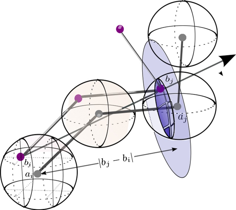
Approximating T_opt(b_i) and T_opt(b_j).

In the following paragraphs, we describe the three components of our algorithm, i.e., the existence of a nearly optimal transformation given a radial axis alignment of B_opt, identify a nearly optimal radial axis alignment, and how to calculate the optimal rotation given a radial axis alignment (Table 1).

Table 1.

Distance Approximation Algorithm for LWPS(A, B, d)

Input:	Structure A, Model B, threshold d, and constant ε
Output:	a transformation T, and matching set M
1.	foreach index
	/* using 〈bi, bj〉 as radial axis candidate of Bopt */
2.	discretize the d-ball C of ai with a grid of side length1/3εd;
	foreach grid point of C
	discretize the sphere cap D with grids of side length c2εd.
	D is defined by the portion of the -sphere of
	encapsulated inside the d-ball of aj.
	foreach grid point of D
	calculate a transformation T to map 〈bi, bj〉 to
3.	applyT to B;
	/* using 〈bi, bj〉 as rotation axis */
	foreach
	determine the angle interval Rk that brings bk into the d-ball of ak;
	endfor
	use plane-sweep algorithm to find a angle γ
	covered by the maximum number of intervals
	endfor
	endfor
	endfor
	return the largest γ, the corresponding radial axis transformation, rotation angle and matching set.

2.3.1. Existence of nearly optimal transformation given a nearly optimal radial axis alignment

Let be an optimal transformation of protein structure B, and let 〈b₁, b₂〉 be the radial axis in B. Suppose we are able to find an approximation T′ for such that and , then we claim that there exists a rotation R around the axis along , that transforms every point to some point near . Formally,

Lemma 1.

Given a point set B, rigid transformations , and T′, let 〈b₁, b₂〉 be a radial axis of B, if and , then there exists a rotation R around the axis along such that .

 Proof. Denote and . With two points fixed, the only degree of freedom for a rigid transformation T′ on B are rotations around the axis along . Therefore we just need to show that there exists a transformation T″ which transforms such that coincides with , and coincides with , and .

We consider T″ as follows, in two steps. First, we translate with translation t such that coincides with T′(b₁). Second, we rotate with rotation axis as the line which passes though and is orthogonal to the plane defined by points , and , with rotation angle as the angle formed by , and , where is the vertex. Denote this rotation as R″ and the rotation angle as α. It can be verified that and . With rotation R″, we move to coincide with .

By translation t, we know that . As , we have . Consider the triangle formed by , and , where is the vertex, we know that (1) the angle formed by points , and with as the vertex is at most α; and (2) . By these two properties, we have . Therefore, by triangle inequality we have . The statement holds.  ■

2.3.2. Finding a nearly optimal radial axis alignment

If we know a radial axis 〈b_i, b_j〉 of B_opt matches to the pair 〈a_i, a_j〉 of A, then we have and .

As shown in Figure 1, we partition the d-ball of a_i with 3D grids of side length 1/3εd. The number of grid points to partition the d-ball of a_i is bounded by O(d³/(1/3εd)) = O(1/ε³). Here we can try all the grid positions for b_i.

Once we have fixed b_i at a grid point, all the possible positions for b_j fitting into the d-ball a_j form a sphere cap centered at b_i with radius and contained in the d-ball of a_j. The spherical cap has an area of O(d²). We partition the sphere cap with grids of resolution size 1/ε. This can be approximated by creating the smallest cube which encapsulates the sphere (the one the sphere cap belongs to) and create grids of side length O(1/ε) of the six faces of the cube. Then we can use the grid on the cube to partition the sphere cap—a common trick used in computation geometry to round the directions (Agarwal et al., 1992). Note that we do not need to create the grid explicitly. It is easy to show that only O(1/ε²) grid points are necessary to partition the sphere cap.

Combining with Lemma 3, to be shown later, we have the following result.

Lemma 2.

If we know a radial axis 〈b_i, b_j〉 of B_opt matching to a pair 〈a_i, a_j〉 of A, there are O(1/ε⁵) possible choices to transform 〈b_i, b_j〉 such that at least one of the transformations results in error at most εd for each from their optimal positions.

2.3.3. Finding the optimal rotation given a good radial axis alignment

Suppose all the points of B must be rotated around a given axis, we want to identify an angle such that the number of matched pairs is maximized. If we represent the interval [0, 2π) as a unit circle, then it is not difficult to see that the angle that moves b_i into the d-ball of a_i form an arc of the circle. There are O(n) arcs in total. Each arc consists of two endpoints, and the circle is subdivided into O(n) circular intervals. Each of these intervals consists of a set of equivalent rotation angles and we can simply pick up an angle contained in the interval to represent the interval. The problem is equivalent to that of finding a point on the circle covered by the maximum number of arcs and it can be solved by the algorithm with a plane-sweep approach (Alt et al., 1987; Choi and Goyal, 2006).

Lemma 3.

The LWPS(A, B, d) problem can be solved in time O(n log n) when rotations are allowed only on a given rotation axis.

As we do not know which pair is a radial axis of B_opt, we enumerate all the possible cases. There are O(n²) possible cases. For two pairs 〈b_i, b_j〉 and 〈a_i, a_j〉, we have ways to match them. For each discretizaion we need time O(n log n) to find the best match by Lemma 3. Therefore, we have the following result:

Theorem 2.

The LWPS(A, B, d) can be solved in time with a d/(1 + ε) distance approximation algorithm.

2.4. An efficient randomized algorithm for globular protein structure

The distance approximation algorithm proposed in Theorem 2 has a time complexity of O(n³ log n), which is still inefficient. If we know a radial axis 〈b_i, b_j〉 of B_opt, then we can solve the problem in time . This observation inspires us to improve the algorithm by identifying a radial axis 〈b_i, b_j〉 or some pair good enough to approximate a radial pair. This section presents an efficient method to identify such a pair with high probability for meaningful models of globular proteins.

A model is meaningful if the TMScore is greater than 0.4 (Zhang and Skolnick, 2004). Here TMScore is defined as:

where d_i is the Euclidean distance between a_i and b_i under the transformation, d has a similar meaning as in the present article, which is a predefined threshold, and M′ is a subset of [1, n].

Immediately, we can prove that M′ has a size of at least 0.4n. A careful analysis of Zhang and Skolnick (2004) will show that M′ has a subset of at least 0.1n matched pairs with distance less than d for a meaningful match. Therefore, the following assumption is reasonable:

Assupmption 1.

A meaningful prediction B of structure A has αn, for some constant α.

We call a pair of points b_i and b_j a pseudo radial pair if . We create grids of side length 1/3(1/2α)^1/3 εd, recall that for globular proteins R_B = n^1/3. If we use pseudo radial axes as a radial axis, the error introduced at each point in the matching set is less than:

Therefore, we can make the following statement:

Lemma 4.

Given a globular protein P, rigid transformations and T′, let 〈p₁, p₂〉 be a pseudo radial axis of P, if and , then there exists a rotation R around the axis along , such that , where c is some constant.

The proof is omitted. Thus, any pseudo radial axis gives us a (1 + ε) distance approximation algorithm.

Theorem 3.

There exists a probabilistic d(1 + ε) distance approximation algorithm for LWPS for globular proteins of meaningful models with probability at least 1 − O(1/n) in time .

We first prove that there exist enough radial axes.

Lemma 5.

B_opt contains at least 1/2 |B_opt|² pairs b_i and b_j such that |b_i − b_j | ≥ (1/2 αn)^1/3.

Proof. The number of points confined in the ball centered at p with radius (1/2αn)^1/3, is bounded by 1/2αn. This implies that there are at least |B_opt| − 1/2αn points in B_opt with a distance at least (1/2αn)^1/3. Thus, the statement holds.  ■

Since there are at least 1/2(αn)² pseudo radial axes, randomly sampling ⌈1/α² log n⌉ pairs from B yields a randomized distance approximate algorithm. Note that each pair has a probability of being a pseudo radial axis. Given that there are ⌈1/α² log n⌉ pairs, the probability that none of them is a pseudo radial axis is O(1/n). In addition, calculation for each pair needs time O(n log n/ε⁵), thus the total time complexity is O(n log² n/ε⁵).

2.5. Approximating the bottleneck distance

In some cases, we need to compute the minimum distance d* such that each point b_i in B can fit into the corresponding d*-ball of a_i, . Techniques by Alt et al. (1987) can be used to address this problem; however, these techniques suffer from high time complexities. We present in this section an efficient method.

First, we investigate the problem if we have some d′ such that d′ ≤ d_opt ≤ 2d ′. We have the following fact:

Lemma 6.

If d′ ≤ d_opt < 2d′, we can approximate d_opt with ratio (1 + ε) in time .

Proof. We subdivide interval [d′, 2d′] into intervals of length 0.5εd′ (assume 1 is divisible by 0.5ε). There are 2/ε such intervals in total. For each interval , we build grids of side length 1/3εd′ for (1 + 0.5(i + 1)ε)d′-ball of a_i, 1 ≤ i ≤ n. Then we check if there is a transformation specified by such grids to fit all the points. For two consecutive intervals λ_i and λ_i + 1, if there is a feasible solution for interval i + 1, and it is infeasible for interval i + 1, then we know that . This yields a (1 + ε)d_opt algorithm immediately. We can use a binary search to find such i, which needs O(log 1/ε) search operations.

In addition, for each search operation, it will be expensive if we employ the enumerating techniques proposed in the previous sections. Instead, we notice that any radial axis of B can be used as we want to fit all the points. In total, there are O(1/ε⁵) possible choices for a given radial axis. Given a rotation axis, the angle to fit b_i into a_i can be modeled as an arc on a circle as previously, and we just need to check if there is a point on the circle covered by n arcs, this can be done in O(n) time.

Thus, each search operation can be performed in time O(n/ε⁵).  ■

Now the remaining difficulty is to find a d′ meeting the requirement d′ ≤ d_opt < 2d ′. We make use of RMSD to achieve this goal. RMSD can be computed in linear time (Arun et al., 1987). RMSD is defined as the minimal root mean square deviation over all the possible transformation I, i.e.,

Let , according to the definition of RMSD, we can prove:

Lemma 7.

Proof. First, we prove that . Suppose , and let I′ be the transformation to obtain d_opt, then we have: . This contradicts the definition of RMSD.

Second, we prove , let I* be the transformation to obtain the RMSD distance:

  ■

We subdivide interval into intervals , 0 ≤ i ≤ 1/2 log n − 1 (assume 1/2 log n is an integer, WLOG). For each interval, we build grids of side length and ball of radius . If there is a feasible solution under such grids, then we know that . We can perform a binary search similar to the previous one to find such i.

Thus we have the following result:

Theorem 4.

The bottleneck distance can be approximated with ratio (1 + ε)d_opt in time

3. Results

We implemented the algorithm in Theorem 2, resulting in a program called OptGDT. The implementation has been done carefully to avoid redundant computations. First, given pairs 〈b_i, b_j〉and 〈a_i, a_j〉, let . If or , we simply preclude 〈b_i, b_j〉 as a radial axis candidate, as it is impossible for b_i to match a_i and b_j to match a_j simultaneously. Second, given a radial axis candidate 〈b_i, b_j〉, we compute an upper bound for all the O(ε⁵) axis under pair 〈b_i, b_j〉 by employing the approximation algorithm in Choi and Goyal (2006). If the bound is smaller than the best solution that we have found so far, there is no need to explore any further for the pair 〈b_i, b_j〉. Third, we try to explore the pairs which are more likely to be the best solution first. We also employed other rules to accelerate our program.

To investigate the performance of OptGDT, we first investigate the superpostion yielded by OptGDT on two concrete examples, and perform comparison with the original GDT. Then we test OptGDT on CASP8 data. In particular, we use the models predicted by the top ten servers in (CASP8, 2008). We use the first model reported by each server. There are 172 domains. Most of the servers predicted results for each domain, resulting in a total of 1714 models reported for all the domains. In all the computation, we set ε = 0.1.

3.1. Two concrete examples by OptGDT

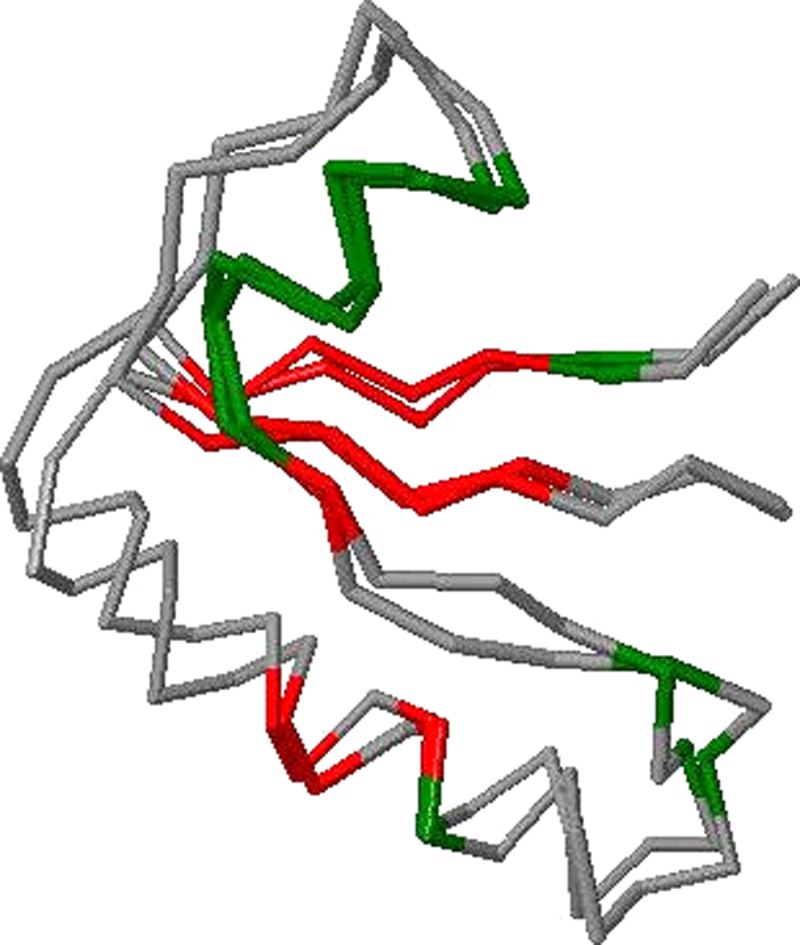
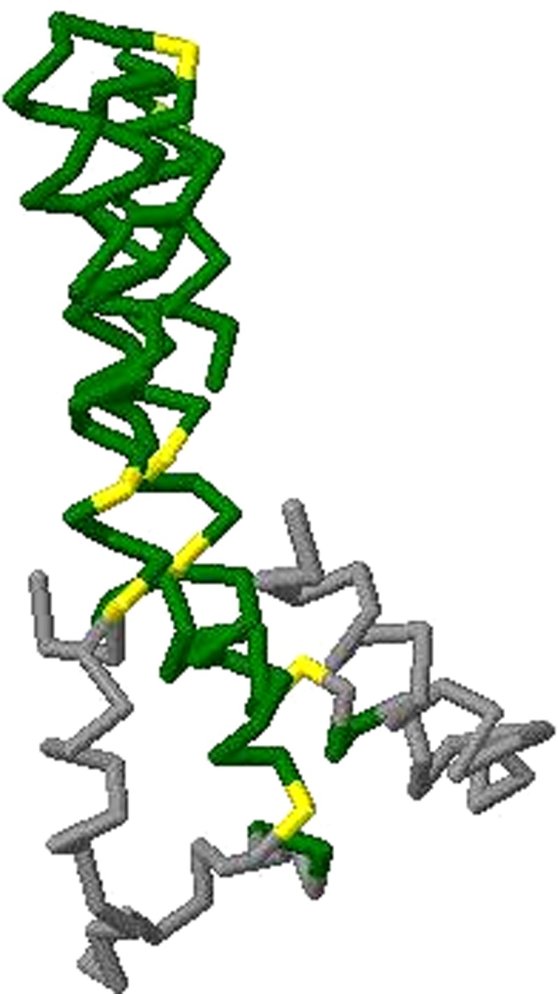
We first show two concrete instances which demonstrate that OptGDT can find better superpositions. Superpositions from computing GDT1 using, respectively, the original method for GDT computation and OptGDT can be obtained (Figs. 2 and 3). The model reported was by BAKER-ROSETTA for the target T0490, domain 2. There are 56 residues, and the residue numbers are from 88 to 143. The GDT1 score obtained by the original method is 0.3393, and that obtained by OptGDT is 0.4464. The increment is more than 0.1. The matched residues by the original method are the residues numbered 90, 95, 108, 110, 114–115, 117, 122–129, 131, 135–136, and 140. The matched pairs by OptGDT are the residues numbered 90–96, 104–105 107–108, 115, 117, 121–130, and 137–140. For clarity the superpositions have been color-coded. The green parts correspond to the matched pairs common to the superpositions from both methods. The yellow parts are the pairs matched only in the original method's superposition. The red parts are the pairs matched only in OptGDT's superposition.

FIG. 2.

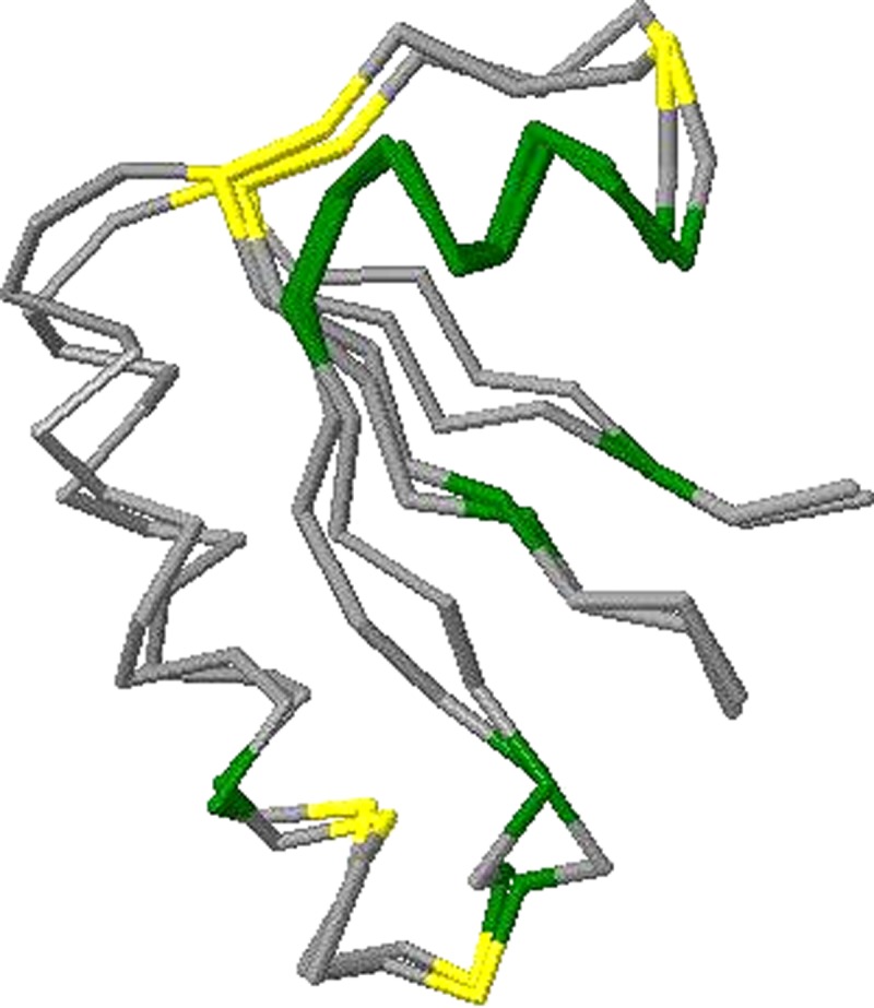
Superpositions of GDT1 by Original GDT for T0490, domain 2 for BAKER-ROBETTA.

FIG. 3.

Superpositions of GDT1 by OptGDT for T0490, domain 2 for BAKER-ROBETTA.

3.2. Performance of OptGDT on CASP8 data

We first compare the original total GDT scores of each server with the total GDT scores computed by OptGDT. The TMScore program has implemented the TMScore, MaxSub Score, RMSD, and GDT scores computation. We use GDT computation in the TMScore program for illustration. For the comparison to the GDT scores computed by LGA (Zemla, 2003), please refer to the software website.

Table 2 shows the scores. The servers are sorted according to the GDT scores obtained by OptGDT. The total score of each server is increased by at least two. Therefore, on average, the GDT score for each domain is increased by at least 0.011. The ranks of some servers are altered due to the more accurate GDT score computation. The reordered servers are MULTICOM-REFINE, MULTICOM-CLUSTER and Phyre_de_novo.

Table 2.

Traditional GDT Scores and OptGDT GDT Scores

	Orig. GDT		New GDT
Serves	GDT	Rank	OptGDT	Rank
Zhang-Server	114.58	1	116.79	1
RAPTOR	110.70	2	112.71	2
pro-sp3-TASSER	109.83	3	112.38	3
BAKER-ROBETTA	109.23	4	111.60	4
MULTICOM-REFINE	108.46	7	110.79	5
MULTICOM-CLUSTER	108.56	6	110.77	6
Phyre_de_novo	108.56	5	110.72	7
MUProt	108.32	8	110.65	8
MULTICOM-RANK	107.03	9	109.22	9
PS2-server	104.30	10	106.62	10

Column 1, server name; column 2, sum of original GDT scores for CASP8 data; column 3, rank according to the original GDT scores; columns 4 and 5, GDT scores and rank by OptGDT, respectively.

3.3. More accurate score computation

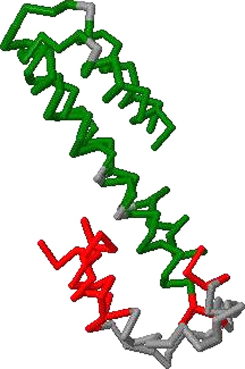
OptGDT is able to improve on many of the original GDT scores computed for the predicted models. Table 3 shows the number of models with changes in score which exceed a specified value. We notice that among 1714 models, 1497 models have their scores increased, which is more than 87.3%. The rest remains unchanged. Larger changes are observed for GDT1 and GDT8 than for GDT2 and GDT4 (Figs. 4 and 5).

Table 3.

Number of Models with Score Increased More than a Certain Constant

	GDT1	GDT2	GDT4	GDT8	GDT
>0.08	4	0	0	22	0
>0.07	20	0	2	46	0
>0.06	34	1	6	58	0
>0.05	90	20	26	93	4
>0.04	184	66	73	139	9
>0.03	441	202	219	227	54
>0.02	862	510	497	371	376
>0.01	1284	1011	979	678	1085
>0	1383	1183	1151	825	1497
= 0	331	531	563	889	217

Columns 2–6, number of models with score change satisfy the condition specified by the first column.

FIG. 4.

Superpositions of GDT8 by Original GDT for T0496, domain 2 for Zhang-Server.

FIG. 5.

Superpositions of GDT8 by OptGDT for T0496, domain 2 for Zhang-Server.

4. Conclusion

We have proposed approximation algorithms with accuracy guarantees for computing GDT, a popular measure for evaluating predicted protein models, and implemented one of these algorithms into an efficient and practical software package called OptGDT. The software package can be used to verify GDT values computed using other heuristic methods, as well as to identify better superpositions in GDT computation.

Experiments on models predicted in CASP8 showed that GDT scores were underestimated and better superpositions are possible for most of the models. In some cases, the scores incremented by more than 10%. The ranks of a few servers were altered due to the more accurate GDT scores. We are convinced that impartial tools to assess predicted models are necessary, and that more accurate superpositions can give us better insights on the structural prediction methods being studied.

Our techniques can also be applied to the protein structure alignment problems. However, the results are of mainly theoretical interests due to their high time complexities.

Acknowledgments

We thank Yen Kaow Ng for helpful discussions. This work was made possible by the facilities of the Shared Hierarchical Academic Research Computing Network (SHARCNET: www.sharcnet.ca). This work was partially supported by the NSERC (grant OGP0046506), China's Ministry of Science and Technology (863 grant 2008AA02Z313), Canada Research Chair program, MITACS, an NSERC Collaborative Grant, and the Cheriton Scholarship.

Disclosure Statement

No competing financial interests exist.

References

- Agarwal P.K. Matoušek J. Suri S. Farthest neighbors, maximum spanning trees and related problems in higher dimensions. Comput. Geom. Theory Appl. 1992;1:189–201. [Google Scholar]
- Alt H. Mehlhorn K. Wagener H., et al. Congruence, similarity, and symmetries of geometric objects. Proc. SCG ’87. 1987:308–315. [Google Scholar]
- Ambühl C. Chakraborty S. Gärtner B. Computing largest common point sets under approximate congruence. Proc. ESA ’00. 2000:52–63. [Google Scholar]
- Arun K.S. Huang T.S. Blostein S.D. Least-squares fitting of two 3-D point sets. IEEE Trans. Pattern Anal. Mach. Intell. 1987;9:698–700. doi: 10.1109/tpami.1987.4767965. [DOI] [PubMed] [Google Scholar]
- CASP8. 8th community wide experiment on the critical assessment of techniques for protein structure prediction. Available at: http://predictioncenter.org/casp8/ Accessed October. 2008;1:2010. [Google Scholar]
- Choi V. Goyal N. A combinatorial shape matching algorithm for rigid protein docking. Proc. CPM. 2004:285–296. [Google Scholar]
- Choi V. Goyal N. An efficient approximation algorithm for point pattern matching under noise. Proc. LATIN 2006. 2006:298–310. [Google Scholar]
- Kolodny R. Linial N. Approximate protein structural alignment in polynomial time. Proc. Natl. Acad. Sci. USA. 2004;101:12201–12206. doi: 10.1073/pnas.0404383101. [DOI] [PMC free article] [PubMed] [Google Scholar]
- Lancia G. Istrail S. Protein structure comparison: algorithms and applications. Math. Methods Protein Struct. Anal. Design. 2003:1–33. [Google Scholar]
- Siew N. Elofsson A. Rychlewski L., et al. Maxsub: an automated measure for the assessment of protein structure prediction quality. Bioinformatics. 2000;16:776–785. doi: 10.1093/bioinformatics/16.9.776. [DOI] [PubMed] [Google Scholar]
- Zemla A. LGA: a method for finding 3D similarities in protein structures. Nucleic Acids Res. 2003;31:3370–3374. doi: 10.1093/nar/gkg571. [DOI] [PMC free article] [PubMed] [Google Scholar]
- Zhang Y. Skolnick J. Scoring function for automated assessment of protein structure template quality. Proteins. 2004;57:702–710. doi: 10.1002/prot.20264. [DOI] [PubMed] [Google Scholar]