Effect of electric potential and current on mandibular linear measurements in cone beam CT

Abstract

Objectives

The purpose of this study was to compare mandibular linear distances measured from cone beam CT (CBCT) images produced by different radiographic parameter settings (peak kilovoltage and milliampere value).

Methods

20 cadaver hemimandibles with edentulous ridges posterior to the mental foramen were embedded in clear resin blocks and scanned by a CBCT machine (CB MercuRay^TM; Hitachi Medico Technology Corp., Chiba-ken, Japan). The radiographic parameters comprised four peak kilovoltage settings (60 kVp, 80 kVp, 100 kVp and 120 kVp) and two milliampere settings (10 mA and 15 mA). A 102.4 mm field of view was chosen. Each hemimandible was scanned 8 times with 8 different parameter combinations resulting in 160 CBCT data sets. On the cross-sectional images, six linear distances were measured. To assess the intraobserver variation, the 160 data sets were remeasured after 2 weeks. The measurement precision was calculated using Dahlberg's formula. With the same peak kilovoltage, the measurements yielded by different milliampere values were compared using the paired t-test. With the same milliampere value, the measurements yielded by different peak kilovoltage were compared using analysis of variance. A significant difference was considered when p < 0.05.

Results

Measurement precision varied from 0.03 mm to 0.28 mm. No significant differences in the distances were found among the different radiographic parameter combinations.

Conclusions

Based upon the specific machine in the present study, low peak kilovoltage and milliampere value might be used for linear measurements in the posterior mandible.

Introduction

When dental implants are to be installed in the posterior part of the mandible, vital structures such as the mandibular canal and mental foramen must be localized to avoid any injury to the neurovascular bundle.^1,2 Panoramic radiography has been used to find the distance between the alveolar bone crest and the superior border of the mandibular canal.^3-7 Conventional tomography has been implemented to visualize not only the superoinferior and anteroposterior dimensions but also the buccal-lingual dimension of the mandible.^8-11 In the late 1990s, cone beam CT (CBCT) was introduced into dentistry. The benefit of CBCT over panoramic radiography is the capability to display three-dimensional images. CBCT is gradually replacing conventional tomography. This is because CBCT can demonstrate sharper images and show volume rendering. Also, patient positioning in CBCT is easier than in conventional tomography. Although fan beam CT can provide similar radiographic outcomes as CBCT,¹² the radiation exposure to the patient from fan beam CT is higher than that from CBCT.^12-15 The accuracy of linear measurements obtained with CBCT for pre-operative planning of implant placement has been reported to be reliable in the posterior mandible.^16,17 In spite of the high accuracy of the radiographic modality, the risk from ionizing radiation must be taken into account prior to prescribing patients to radiographic examination. According to the most accepted principle, ALARA (as low as reasonably achievable), the minimum radiation exposure is implemented to achieve adequate radiographic information.^18,19 Radiation dose in CBCT can be reduced by lowering the radiographic parameters, such as the peak kilovoltage and milliampere value,²⁰ field of view (FOV)²¹ and scan time. However, the noise, a physical property in CBCT, increases with decreasing beam current.²² Based on subjective evaluation, significant reduction in peak kilovoltage and milliampere value did not substantially affect overall image quality.^23,24 Various radiation doses from four CBCT scanners rendered different image qualities in terms of segmentation accuracy.²⁵ The requisites of image quality change according to the various types of examination or even various purposes within the same examinations.²⁶ An important task performed using CBCT images of the mandible in implant patients is to objectively measure the linear distances in the cross-sectional views. The effect of radiographic settings, i.e. peak kilovoltage and milliampere, on mandibular linear measurements in CBCT images has not been objectively studied. The purpose of this study was to compare mandibular linear distances measured on CBCT images produced by different radiographic parameters.

Materials and methods

The study protocol was approved by the Ethics Committee for dental research, Faculty of Dentistry, Chulalongkorn University. 20 hemimandibles were collected from the Department of Anatomy, Faculty of Dentistry, Chulalongkorn University. Only the hemimandibles with an edentulous ridge posterior to the mental foramen were included. The age of the individuals ranged from 56 years to 92 years, with a mean of 77.21 ± 7.55 years. The female-to-male ratio was 2:3. The hemimandibles were embedded in clear resin blocks with the lower border of the mandible parallel to the horizontal plane (Figure 1). The resin blocks were 3.5×5 × 10 cm and were used to simulate the soft-tissue components. A CBCT machine (CB MercuRay^TM; Hitachi Medico Technology Corp., Chiba-ken, Japan) was used to scan the hemimandibles. The radiographic parameters consisted of four peak kilovoltage settings (60 kVp, 80 kVp, 100 kVp and 120 kVp) and two milliampere settings (10 mA and 15 mA). An FOV of 102.4 mm was chosen to scan the hemimandibles, since this FOV is recommended by the manufacturer for dental implant patients. The resultant isotropic voxel size was 0.2 mm. The scan time was 14 s. Each hemimandible was scanned eight times with eight different setting combinations (60 kVp and 10 mA, 60 kVp and 15 mA, 80 kVP and 10 mA, 80 kVp and 15 mA, 100 kVp and 10 mA, 100 kVp and 15 mA, 120 kVp and 10 mA, and 120 kVp and 15 mA). 160 CBCT data sets were acquired by CB Works proprietary software v. 2 (Cybermed, Seoul, Republic of Korea). The first generation of reconstructed data sets with spatial resolution of 512 × 512 pixels and grey resolution of 12 bits (4096 shades of grey) were transferred to a picture archiving and communication system. Multiplanar reformatted images, i.e. separate stacks of coronal, axial and sagittal tomographic images with slice thickness of 0.2 mm were reconstructed by Infinitt proprietary software v. 2 (Infinitt Co., Seoul, Republic of Korea) and shown simultaneously on a 20.8 inch monochrome monitor (Totoku ME355i2, Totoku Electric Co., Tokyo, Japan) with a spatial resolution of 2048 × 1536 pixels and greyscale of 11 bits (2048 shades of grey). No filtering was used. To assure that the same coronal slice of the hemimandible was measured for all the peak kilovoltage/milliampere combinations, each resin block was placed in the scanning machine at the same position for all combinations. In the axial image of the multiplanar reformation screen obtained using 120 kVp/15 mA, the long axis of the hemimandible was situated vertically on the screen. The stack of axial images of the hemimandible was reviewed slice by slice from the lower border of the mandible. The slices were reviewed until the buccal cortex in the area of mental canal became discontinuous. The reviewing went further up slice by slice until the anterior border of the mental foramen was well delineated. The number of slices from the slice where the buccal cortex became discontinuous to the slice where the anterior border of the mental foramen was well delineated was recorded. This latter axial slice was captured as the reference image, particularly concerning the configuration of the anterior border of the mental foramen for the other seven peak kilovoltage/milliampere combinations. The aforementioned number of slices was used to select the axial slice for the other seven peak kilovoltage/milliampere combinations. In the selected axial slice of the 120 kVp/15 mA combination, a 10 mm vertical line was drawn from the anterior border of the mental foramen posteriorly. The coronal slice 10 mm behind the anterior border of the mental foramen was examined for the location of the mandibular canal. Then the location of the mandibular canal in the coronal slices was reviewed from the mental foramen to the posterior part of the mandible and vice versa to confirm the location of the mandibular canal. The coronal slices at a distance of 10 ± 2 mm behind the anterior border of the mental foramen were reviewed back and forth, and the slice with the best delineated mandibular canal border was selected for measurements. In two hemimandibles, the location of the mandibular canal could not be definitively located. In these samples, the border of the mandibular canal was subjectively identified in the coronal slices within the distance of 10 ± 2 mm behind the anterior border of the mental foramen. Once the coronal slice of the 120 kVp/15 mA combination was selected, the distance behind the anterior border of the mental foramen indicating the location of the coronal slice for measurements was used for locating the coronal slice of the other seven peak kilovoltage/milliampere combinations. On the selected coronal images, six linear distances were measured, i.e. the distances between the inner surface of the superior wall of the mandibular canal and the horizontal level of the alveolar crest (Up), the inner surface of the lower wall of the mandibular canal and the horizontal level of the lower border of the mandible (Lo), the inner surface of the buccal wall of the mandibular canal and the buccal border of the mandible (Bu), the inner surface of the lingual wall of the mandibular canal and the lingual border of the mandible (Li), and the vertical (V) and horizontal (H) widths of the mandibular canal measured between the inner surfaces of the canal wall (Figure 2). During measuring, the observer (SP), who had been working with CBCT for 5 years, could adjust the image density, contrast and magnification until the images were subjectively regarded as the images of best clarity. The stacks of the tomographic images could be reviewed back and forth to confirm the outline of the mandibular canal. Each distance was measured three times and the average was used. Therefore, 2880 (20 specimens × 8 settings × 6 distances × 3 times) measurements were performed. 160 data sets were measured on a second occasion 2 weeks after the first occasion by the same observer. Measurement precision was calculated using the first measurement and the repeated measurement after 2 weeks and expressed as standard deviation (SD) according to Dahlberg's formula, which is SD = where d is the difference between the two measurements and n is the number of duplicated measurements.²⁷ Measurement precision was acquired separately for each of the peak kilovoltage/milliampere combinations. With the same peak kilovoltage, the measurements yielded by different milliampere values were compared using the paired t-test. With the same milliampere value, the measurements yielded by different peak kilovoltage were compared using one-way analysis of variance. Descriptive statistics were calculated with Excel 2003 (Microsoft, Redmond, WA). Statistical analysis was performed with the use of SPSS® v. 11 (SPSS, Chicago, IL). A significant difference was considered when p < 0.05.

Figure 1.

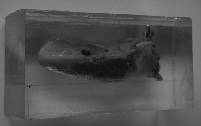
A hemimandible embedded in a clear resin block with the lower border of the mandible parallel to the horizontal plane. The size of the block was 3.5 × 5 × 10 cm

Figure 2.

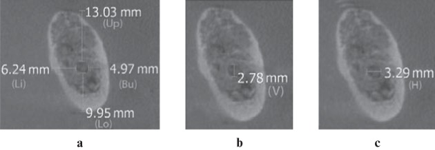
Cross-sectional images demonstrating the six mandibular linear distances. (a) Up, distance between the inner surface of the superior wall of the mandibular canal and the horizontal level of alveolar crest; Lo, inner surface of the lower wall of the mandibular canal and the horizontal level of the lower border of the mandible; Bu, inner surface of the buccal wall of the mandibular canal and the buccal border of the mandible; Li, inner surface of the lingual wall of the mandibular canal and the lingual border of the mandible. (b) V, vertical width of the mandibular canal. (c) H, horizontal width of the mandibular canal

Results

The precision of the measurements ranged from 0.03 mm to 0.28 mm (Table 1). The means and SDs of the 6 mandibular linear distances of the 20 hemimandibles are presented in Table 2 with regards to different combinations of peak kilovoltage and milliampere values. With the same peak kilovoltage, the measurements yielded by different milliampere settings (10 mA and 15 mA) were not significantly different. With the same milliampere value, the measurements yielded by different peak kilovoltage (60 kVp, 80 kVp, 100 kVp, and 120 kVp) were not significantly different.

Table 1. Measurement precision in millimetres of mandibular distances of the 20 hemimandibles relative to various combinations of peak kilovoltage and milliampere.

kVp, mA	Up	Lo	Bu	Li	V	H
60, 10	0.08	0.09	0.1	0.11	0.1	0.05
60, 15	0.06	0.05	0.05	0.08	0.07	0.09
80, 10	0.06	0.05	0.03	0.1	0.07	0.08
80, 15	0.08	0.05	0.05	0.07	0.08	0.08
100, 10	0.06	0.06	0.04	0.05	0.08	0.1
100, 15	0.09	0.09	0.1	0.15	0.1	0.09
120, 10	0.09	0.10	0.1	0.11	0.11	0.1
120, 15	0.18	0.12	0.15	0.14	0.28	0.2

kVp, peak kilovoltage; mA, milliampere; Bu, distance between buccal border of mandibular canal and buccal border of mandible; H, horizontal width of the mandibular canal; Li, lingual border of mandibular canal and lingual border of mandible; Lo, lower border of mandibular canal and horizontal level of lower border of mandible; Up, superior border of mandibular canal and horizontal level of alveolar crest; V, vertical width of the mandibular canal.

Table 2. Mean ± standard deviation in millimetres of mandibular distances of the 20 hemimandibles relative to various combinations of peak kilovoltage and milliampere.

kVp, mA	Up	Lo	Bu	Li	V	H
60, 10	10.48 ± 4.23	8.13 ± 1.51	6.09 ± 1.19	3.47 ± 1.20	2.59 ± 0.54	2.84 ± 0.39
60, 15	10.57 ± 4.30	8.40 ± 1.39	6.22 ± 1.17	3.27 ± 1.08	2.44 ± 0.47	2.72 ± 0.47
80, 10	10.68 ± 4.25	8.31 ± 1.21	6.19 ± 1.22	3.21 ± 1.10	2.47 ± 0.46	2.67 ± 0.37
80, 15	10.73 ± 4.27	8.37 ± 1.39	6.22 ± 1.06	3.31 ± 1.54	2.51 ± 0.36	2.61 ± 0.42
100, 10	10.68 ± 4.31	8.53 ± 1.28	6.08 ± 1.39	3.35 ± 1.39	2.45 ± 0.57	2.60 ± 0.58
100, 15	10.66 ± 4.23	8.44 ± 1.25	5.95 ± 1.37	3.47 ± 1.28	2.58 ± 0.52	2.52 ± 0.50
120, 10	10.66 ± 4.33	8.39 ± 1.16	5.87 ± 1.39	3.44 ± 1.22	2.69 ± 0.60	2.54 ± 0.38
120, 15	10.67 ± 4.26	8.40 ± 1.24	5.97 ± 1.32	3.30 ± 1.19	2.66 ± 0.43	2.58 ± 0.41

Bu, distance between buccal border of mandibular canal and buccal border of the mandible; H, horizontal width of the mandibular canal; Li, lingual border of mandibular canal and lingual border of mandible; Lo, lower border of mandibular canal and horizontal level of lower border of mandible; Up, distance between superior border of mandibular canal and horizontal level of alveolar crest; V, vertical width of the mandibular canal.

Discussion

The first step in linear measurement is to identify the landmarks that make up the measurement.²⁸ Reliability in identifying landmarks is affected by several factors, such as the clarity of the definition describing the landmark, the quality of the image, the geometry of the object to be identified and the image contrast between adjacent objects.²⁸ In the present study, the border of the mandibular canal was defined at the inner surface of the canal wall where the radio-opaque density of the canal wall was highly contrasted against the radiolucent density of neurovascular bundles. This probably contributed to reliability in identifying landmarks. The quality of the image, in terms of density, contrast and magnification, which was adjusted until the subjectively best clarity of the image was obtained, was probably another contributing factor to reliability in identifying landmarks.

In a recent study by Kwong et al,²³ it was postulated that soft tissue had an effect on the image quality when various exposure settings were used. The present study did not reveal any effect of the soft-tissue simulator made from acrylic resin on linear measurements. This might be due to the different methods used. Another reason might be that different thicknesses of soft-tissue simulator were used.

Recently, it was reported that body mass index, i.e. weight in kilograms divided by height in square metres, did not negatively affect image quality of CBCT.²⁹ However, the effect of the thickness of the soft tissue and bone and the bone density on the image quality of CBCT has not been investigated. Sex also did not influence the diagnostic quality of CBCT images.²⁹ The image quality of the mandibular canal was negatively affected by age.²⁹ The hemimandibles in the present study were from individuals with a mean age of 77.21 ± 7.55 years. We found localizing the mandibular canal difficult in some images. This might have been due to the decrease of bone mineral in old age. Lindh et al⁴ found that the compact bone surrounding the neurovascular bundle was missing in some histological sections of edentulous mandibles, with the result that the canal could not be identified in radiographs. In the same study a large variation was found between observers in identifying the mandibular canal. However, CT showed the least number of missing measurements compared with conventional tomographic methods. In the present study one observer measured all distances and the measurement precision was high.

An overall reduction in radiation dose of approximately 62% was acquired by decreasing the peak kilovoltage from 120 kVp to 100 kVp.²⁰ Reducing tube current causes an increase in image noise.^22,24 However, noise could be reduced by the use of a non-linear edge-preserving smoothing filter.³⁰ In clinical circumstances, low tube current is mostly used when a large FOV with a large resultant voxel size is needed, and high tube current is selected when a small FOV with small resultant voxel size is required.²⁰

The present study was performed using a specific CBCT machine that had an image intensifier tube/charge-coupled device combination as image detector, 102.4 mm FOV and specific radiographic settings. Despite using a specific CBCT machine, the results of the present study could be regarded as a general trend.

In conclusion, based on the results of the present study using a 102.4 mm FOV and certain radiographic settings, reducing both electric potential and current to 60 kVp and 10 mA, respectively, might justify the resultant quality of the CBCT images when measuring mandibular linear distances. Further research is needed to determine the optimal exposure settings to obtain the clinically adequate image quality.

References

- 1.Worthington P. Injury to the inferior alveolar nerve during implant placement: a formula for protection of the patient and clinician. Int J Oral Maxillofac Implants 2004;19:731–734 [PubMed] [Google Scholar]
- 2.Khawaja N, Renton T. Case studies on implant removal influencing the resolution of inferior alveolar nerve injury. Br Dent J 2009;206:365–370 [DOI] [PubMed] [Google Scholar]
- 3.Lindh C, Petersson A, Klinge B. Visualisation of the mandibular canal by different radiographic techniques. Clin Oral Implants Res 1992;3:90–97 [DOI] [PubMed] [Google Scholar]
- 4.Lindh C, Petersson A, Klinge B. Measurements of distances related to the mandibular canal in radiographs. Clin Oral Implants Res 1995;6:96–103 [DOI] [PubMed] [Google Scholar]
- 5.Vazquez L, Saulacic N, Belser U, Bernard JP. Efficacy of panoramic radiographs in the preoperative planning of posterior mandibular implants: a prospective clinical study of 1527 consecutively treated patients. Clin Oral Implants Res 2008;19:81–85 [DOI] [PubMed] [Google Scholar]
- 6.Angelopoulos C, Aghaloo T. Imaging technology in implant diagnosis. Dent Clin North Am 2011;55:141–158 [DOI] [PMC free article] [PubMed] [Google Scholar]
- 7.Kim YK, Park JY, Kim SG, Kim JS, Kim JD. Magnification rate of digital panoramic radiographs and its effectiveness for pre-operative assessment of dental implants. Dentomaxillofac Radiol 2011;40:76–83 [DOI] [PMC free article] [PubMed] [Google Scholar]
- 8.Stella JP, Tharanon W. A precise radiographic method to determine the location of the inferior alveolar canal in the posterior edentulous mandible: implications for dental implants. Part 2: clinical application. Int J Oral Maxillofac Implants 1990;5:23–29 [PubMed] [Google Scholar]
- 9.Ekestubbe A, Grondahl HG. Reliability of spiral tomography with the Scanora® technique for dental implant planning. Clin Oral Implants Res 1993;4:195–202 [Google Scholar]
- 10.Tyndall DA, Brooks SL. Selection criteria for dental implant site imaging: a position paper of the American Academy of Oral and Maxillofacial Radiology. Oral Surg Oral Med Oral Pathol Oral Radiol Endod 2000;89:630–637 [DOI] [PubMed] [Google Scholar]
- 11.Harris D, Buser D, Dula K, Grondahl K, Haris D, Jacobs R, et al. E.A.O. guidelines for the use of diagnostic imaging in implant dentistry. A consensus workshop organized by the European Association for Osseointegration in Trinity College Dublin. Clin Oral Implants Res 2002;13:566–570 [DOI] [PubMed] [Google Scholar]
- 12.Carrafiello G, Dizonno M, Colli V, Strocchi S, Pozzi Taubert S, Leonardi A, et al. Comparative study of jaws with multislice computed tomography and cone-beam computed tomography. Radiol Med 2010;115:600–611 [DOI] [PubMed] [Google Scholar]
- 13.Ludlow JB, Ivanovic M. Comparative dosimetry of dental CBCT devices and 64-slice CT for oral and maxillofacial radiology. Oral Surg Oral Med Oral Pathol Oral Radiol Endod 2008;106:106–114 [DOI] [PubMed] [Google Scholar]
- 14.Okano T, Harata Y, Sugihara Y, Sakaino R, Tsuchida R, Iwai K, et al. Absorbed and effective doses from cone beam volumetric imaging for implant planning. Dentomaxillofac Radiol 2009;38:79–85 [DOI] [PubMed] [Google Scholar]
- 15.Loubele M, Bogaerts R, Van Dijck E, Pauwels R, Vanheusden S, Suetens P, et al. Comparison between effective radiation dose of CBCT and MSCT scanners for dentomaxillofacial applications. Eur J Radiol 2009;71:461–468 [DOI] [PubMed] [Google Scholar]
- 16.Kobayashi K, Shimoda S, Nakagawa Y, Yamamoto A. Accuracy in measurement of distance using limited cone-beam computerized tomography. Int J Oral Maxillofac Implants 2004;19:228–231 [PubMed] [Google Scholar]
- 17.Suomalainen A, Vehmas T, Kortesniemi M, Robinson S, Peltola J. Accuracy of linear measurements using dental cone beam and conventional multislice computed tomography. Dentomaxillofac Radiol 2008;37:10–17 [DOI] [PubMed] [Google Scholar]
- 18.Martin CJ, Sutton DG, Sharp PF. Balancing patient dose and image quality. Appl Radiat Isot 1999;50:1–19 [DOI] [PubMed] [Google Scholar]
- 19.Farman AG. ALARA still applies. Oral Surg Oral Med Oral Pathol Oral Radiol Endod 2005;100:395–397 [DOI] [PubMed] [Google Scholar]
- 20.Palomo JM, Rao PS, Hans MG. Influence of CBCT exposure conditions on radiation dose. Oral Surg Oral Med Oral Pathol Oral Radiol Endod 2008;105:773–782 [DOI] [PubMed] [Google Scholar]
- 21.Pauwels R, Beinsberger J, Collaert B, Theodorakou C, Rogers J, Walker A, et al. Effective dose range for dental cone beam computed tomography scanners. Eur J Radiol 2012;81:267–271 [DOI] [PubMed] [Google Scholar]
- 22.Araki K, Maki K, Seki K, Sakamaki K, Harata Y, Sakaino R, et al. Characteristics of a newly developed dentomaxillofacial X-ray cone beam CT scanner (CB MercuRay): system configuration and physical properties. Dentomaxillofac Radiol 2004;33:51–59 [DOI] [PubMed] [Google Scholar]
- 23.Kwong JC, Palomo JM, Landers MA, Figueroa A, Hans MG. Image quality produced by different cone-beam computed tomography settings. Am J Orthod Dentofacial Orthop 2008;133:317–327 [DOI] [PubMed] [Google Scholar]
- 24.Sur J, Seki K, Koizumi H, Nakajima K, Okano T. Effects of tube current on cone-beam computerized tomography image quality for presurgical implant planning in vitro. Oral Surg Oral Med Oral Pathol Oral Radiol Endod 2010;110:e29–e33 [DOI] [PubMed] [Google Scholar]
- 25.Loubele M, Jacobs R, Maes F, Denis K, White S, Coudyzer W, et al. Image quality vs radiation dose of four cone beam computed tomography scanners. Dentomaxillofac Radiol 2008;37:309–318 [DOI] [PubMed] [Google Scholar]
- 26.Martin CJ, Sharp PF, Sutton DG. Measurement of image quality in diagnostic radiology. Appl Radiat Isot 1999;50:21–38 [DOI] [PubMed] [Google Scholar]
- 27.Dahlberg G. Statistical methods for medical and biological students. New York, NY: Interscience Publications; 1940 [Google Scholar]
- 28.Lou L, Lagravere MO, Compton S, Major PW, Flores-Mir C. Accuracy of measurements and reliability of landmark identification with computed tomography (CT) techniques in the maxillofacial area: a systematic review. Oral Surg Oral Med Oral Pathol Oral Radiol Endod 2007;104:402–411 [DOI] [PubMed] [Google Scholar]
- 29.Ritter L, Mischkowski RA, Neugebauer J, Dreiseidler T, Scheer M, Keeve E, et al. The influence of body mass index, age, implants, and dental restorations on image quality of cone beam computed tomography. Oral Surg Oral Med Oral Pathol Oral Radiol Endod 2009;108:e108–e116 [DOI] [PubMed] [Google Scholar]
- 30.Loubele M, Jacobs R, Maes F, Schutyser F, Debaveye D, Bogaerts R, et al. Radiation dose vs. image quality for low-dose CT protocols of the head for maxillofacial surgery and oral implant planning. Radiat Prot Dosimetry 2005;117:211–216 [DOI] [PubMed] [Google Scholar]