

Abstract
Double Electron–Electron Resonance (DEER) has emerged as a powerful technique for measuring long range distances and distance distributions between paramagnetic centers in biomolecules. This information can then be used to characterize functionally relevant structural and dynamic properties of biological molecules and their macromolecular assemblies. Approaches have been developed for analyzing experimental data from standard four-pulse DEER experiments to extract distance distributions. However, these methods typically use an a priori baseline correction to account for background signals. In the current work an approach is described for direct fitting of the DEER signal using a model for the distance distribution which permits a rigorous error analysis of the fitting parameters. Moreover, this approach does not require a priori background correction of the experimental data and can take into account excluded volume effects on the background signal when necessary. The global analysis of multiple DEER data sets is also demonstrated. Global analysis has the potential to provide new capabilities for extracting distance distributions and additional structural parameters in a wide range of studies.
Keywords: DEER, PELDOR, Global analysis
1. Introduction
With the development of a dead-time-free four-pulse version of the Double Electron-Electron Resonance (DEER) experiment [1] and the production of commercially available instrumentation with DEER capability, the technique has gained wide acceptance particularly in the field of structural biology (for recent reviews of DEER and its biological applications see [2,3]). Given the ability to accurately and precisely measure distances in the 15–80 Å range and the availability of numerous strategies for introducing appropriate spin labels into proteins or oligonucleotides, DEER has been proven particularly useful in studies of structures of both soluble and membrane proteins, structures of biomolecular complexes, and conformational changes associated with biological function.
In a typical DEER experiment, two spin labels are introduced into the object of interest, be it a single biomolecule or macromolecular complex. While in certain circumstances an object such as a homo-oligomeric complex can contain more than two spin labels, in the present work a doubly-labeled object will be assumed. To determine the distance between the two labels within an object, the amplitude of a refocused echo is measured as the timing of a pump pulse at a second microwave frequency is varied. If one of the spins within an object is detected with the refocused echo and the other spin is flipped by the pump pulse, then variations in the timing of the pump pulse will produce variations in the amplitude of the DEER signal.
If the two spins are at a fixed distance, then the modulated DEER signal can be Fourier transformed to give either a full or partial Pake pattern from which the dipolar frequency, ωd,
| (1) |
can be directly read and the interspin distance, R, determined [1]. More typically, significant disorder in both the object itself and in how the spin labels are tethered to the object will result in a distribution of distances, P(R). This disorder also typically removes significant correlation between the distance and relative orientation of the labels. As a result, these correlations can be justifiably ignored when analyzing DEER data to determine P(R). DEER signals are sensitive to important characteristics of P(R) beyond just the mean, 〈R〉, and variance, σR, of the distribution. DEER signals also depend on the number of components or modes (local maxima) in P(R) together with the centers and widths of each component. The goal of any strategy for analyzing DEER data is to extract the most detailed description of the distance distribution from the data.
Two general approaches have been developed for determining a distance distribution from DEER data. The first involves fitting data using either a purely mathematical model [4,5] or a physically based model [6] of P(R). The second uses a mathematical inversion of the DEER signal to generate a model-free P(R) [7-10]. As discussed previously by Fajer and coworkers [4] both approaches have merit. The model-free nature of the inversion methods is highly attractive, but the inversion itself is an ill-posed mathematical problem and additional constraints must be added to make the solution more tractable. Typically, Tikhonov regularization is used to impose a degree of smoothness on P(R).
The analysis of DEER data is complicated by the fact that the DEER signal from the specific dipolar interaction within the object of interest, VO(t), is mixed with a non-specific background signal, VB(t), due to interactions between all of the objects in the sample. The complete signal, V(t), is given by the product of these two contributions [1,7].
| (2) |
In cases where either (1) an experimental background signal has been determined or (2) the functional form of the background signal is known and data has been collected out to a sufficiently long maximum time (tmax), then background correction can be used to obtain a pure VO(t) signal that can be subsequently analyzed to determine P(R). However, the conditions required for proper background correction are not always met in practice due to a variety of factors.
In the first case, samples must be prepared and data collected to experimentally determine VB(t). Collecting these pure background signals from separate samples is time-consuming and in some cases it is not possible to generate the appropriate sample.
In the second case, it is assumed that VO(t) has decayed to a constant value at long values of t. Then, V(t) at these long t values is fit to a known function, typically an exponential decay, to give VB(t). Dividing V(t) by the determined VB(t) gives VO(t). On the other hand, the functional form of the background signal may deviate from the ideal functional form in unpredictable ways. Also, given that significant signal averaging may be required to obtain data with an adequate signal-to-noise ratio (S/N), it is often difficult to determine the appropriate tmax at setup. Due to phase memory relaxation, for a given data acquisition time a longer tmax will give a lower S/N. Thus, there is a bias towards collecting data with shorter tmax which may be insufficient for unambiguous background correction. Finally, an initial time point must be chosen at which to begin fitting V(t) to obtain VB(t). Depending on the choice of a time range to fit for the background signal, significant differences in VO(t) and ultimately P(R) can be obtained. It should be noted that the use of an incorrect background correction can introduce significant artifacts into VO(t). Nonetheless, an excellent fit to VO(t) may be achieved although the distance distribution obtained will necessarily include aspects due to the induced artifacts. All of these factors have motivated the development of an alternative approach to DEER data analysis that does not require a priori background correction.
The DeerAnalysis program developed by Jeschke and coworkers [9] does include the option to fit data without a priori background correction to a unimodal or bimodal Gaussian distance distribution together with a homogeneous background distribution which is equivalent to an exponential background signal. While this model has been successfully used to fit data [e.g. 11,12], the developers of DeerAnalysis strongly discourage the use of this model due to the possibility of becoming trapped in local minima. In the present work, improvements are made in the approach to non-linear least-squares analysis so that the routine fitting of DEER data without a priori background correction is, arguably, now feasible. In addition, an algorithm is developed to treat the excluded volume effect that can affect the background signal of very large objects.
DEER distance measurements can be used to generate new structural models [e.g. 12-16] or to verify existing ones [e.g. 11]. To create or test structural models, it should be sufficient to obtain the average distance, 〈R〉, between labels and possibly the RMSD width of the distribution, σR. DEER can also be used to test for either distance changes [e.g. 17-19] or changes in the population of different components of a distance distribution [e.g. 20-22] that are a result of biologically relevant phenomena. In these studies, results obtained using Tikhonov regularization can be ambiguous. Differences in the P(R) obtained from different samples may be due to actual structural differences or may be artifacts of the inversion process. Recently, some error analysis capabilities have been incorporated into routines for analyzing DEER data using Tikhonov regularization. Nonetheless, direct fitting of the DEER signal using a mathematical model of P(R) can allow for more rigorous error analysis of the parameters defining P(R) and a less ambiguous comparison of results from different samples. In addition, this approach does not require a priori background correction of the data.
In this work, error analysis is performed by the calculation of confidence intervals for the various fit parameters. Confidence intervals consist of a set of additional fits starting at a series of different initial values for a given fit parameter. An added benefit of this approach is that if the initial fit did not reach the global minimum, the calculation of confidence intervals will typically reveal a better fit.
The simultaneous or global analysis of data from multiple experiments collected under different conditions can provide a more rigorous test of the model being used to fit all of the data and a more precise estimate of the model’s parameters. For example in a case where a pair of spin labels was rigidly held in a defined orientation with respect to each other, global analysis of continuous-wave EPR data collected at X-, Q-, and W-bands was used to determine the interspin distance and the relative orientation of the labels [23]. In global analysis, a physical model is defined to fit multiple data sets. Parameters defining the model may either be fixed (not allowed to vary) or floated (allowed to vary) and parameters used to fit different data sets may be linked, i.e. required to have the same value. Thus, different data sets will be fit with the same model and the same parameters.
There are a number of potential applications of global analysis to the fitting of DEER data. Examples include the following:
Data collected at multiple microwave frequency bands.
Data collected over two different time frames: one data set collected at a short tmax with high S/N ratio to better define VO(t) and one collected at a long tmax to define VB(t).
Data collected under different biological or chemical conditions. For example, consider a situation where it is hypothesized that there are two different protein conformers and that binding of a ligand to the protein shifts the equilibrium between the two conformers. DEER data could be collected with and without the ligand and globally analyzed using a bimodal P(R). While the centers and widths of the two components of P(R) would be linked in the global analysis, the relative amplitudes for the two different data sets would be different to account for the shift in the equilibrium.
Data collected from multiple samples labeled at different sites can be combined into a single analysis to determine a desired structure. This approach has been successfully used by Jeschke and coworkers who have fit multiple DEER data sets directly to a structural model [12,14].
Data collected for different pump–probe frequency separations. In highly ordered samples, the angular correlation between the spins is retained and different relative orientations will be selected depending on the frequency difference between the pump and probe pulses. Analysis of DEER data collected at multiple frequency separations can then be used to determine the relative orientation of the two spins [24-26].
In order to demonstrate the potential utility of the global analysis approach developed in this work, data collected at multiple pump–probe frequency separations are analyzed using a simplified model that does not explicitly include orientation. Instead, the data is analyzed in terms of varying fractions of the components in a bimodal distance distribution. The flexibility of the approach developed here for global analysis makes it adaptable to a wide variety of other situations such as those outlined above.
This report describes a program for the GLobal Analysis of DEER Data (GLADD) which has been developed with three goals in mind (1) an ability to fit DEER data without the need for a priori background correction, (2) an ability to perform error analysis on the fit parameters, and (3) a flexible capability to perform simultaneous analysis of data from multiple experiments.
2. Experimental procedures
Procedures for the expression, purification, and spin-labeling of double cysteine mutants of T4 lysozyme (T4L) [27] and single cysteine mutants of the cytoplasmic domain of band 3 protein (CDB3) [11,28] have been previously published. The T4L sample was labeled with (1-oxyl-2,2,5,5-tetramethyl-Δ3-pyrroline-3-methyl) methanethiosulfonate spin label (MTSSL; Toronto Research Chemicals, North York, ON, Canada) and placed in a buffer containing 100 mM NaCl, 20 mM MOPS, 0.1 mM EDTA and 0.02% azide (pH 7.0) with 30% (w/w) glycerol added as a cryoprotectant. The final spin concentration was approximately 0.2 mM. The CDB3 samples were labeled with a perdeuterated 15d-MTSSL (Toronto Research Chemicals) in a D2O buffer containing 20 mM NaH2PO4, 100 mM NaCl, and 1 mM EDTA (pH 6.8) with 30% perdeuterated 8d-glycerol. The final spin concentrations were approximately 0.3 mM.
The four-pulse DEER experiment was performed at X-band using a Bruker EleXsys 580 spectrometer equipped with a Bruker split ring resonator (ER 4118X-MD5). A standard four-pulse sequence was employed with a 32 ns π pulse length and a 16 ns π/2 pulse length. All measurements were recorded at 80 K with samples loaded into 2.4 mm i.d. quartz capillaries (Wilmad LabGlass, Buena, NJ). The pump frequency was set to excite the maximum of the nitroxide spectrum in the mI = 0 manifold, and the observe frequency was set to a higher value to excite the low field mI = +1 manifold. Unless otherwise noted, the difference between the observe and pump frequencies, Δν, was set to 65 MHz.
3. Theory
The goal in this section is to assemble algorithms for fitting the complete DEER signal given in Eq. (2) without the need for a priori background correction. All of the algorithms were developed in MATLAB R2011a (The Mathworks, Inc., Natick, MA, USA) and are available from the corresponding author upon request. As noted above, the DEER signal can be factored into a contribution from the specific dipolar interaction within the object of interest and a background signal. Thus, DEER data is fit using the following equation:
| (3) |
Here, O(t) is the calculated signal for the specific interaction, B(t) is a background signal calculated for a homogeneous three dimensional solution of spheres with a single unpaired electron at the center, and E(t) is an exponential or stretched exponential function. Either B(t) is used as the background signal with E(t) fixed to 1, or the background can be fit as an exponential given by E(t) with B(t) fixed to 1.
3.1. Calculation of O(t)
Following previous authors [7,29,30], the DEER signal for an isolated pair of electron spins assuming ideal pulses is given by
| (4) |
where the angle brackets specify averaging over the appropriate distributions of R and θ, where θ is the angle between the interelectron vector and the magnetic field. The parameter Δ defines the modulation depth and
| (5) |
Assuming that there is no correlation between R and θ then
| (6) |
where
| (7) |
and C and S are the Fresnel cosine and sine integrals.
| (8) |
The integral in Eq. (6) can be solved as a sum over discrete values of R,
| (9) |
Typically, Ri will range from 0 to 100 Å in steps of 0.1 Å. The distance distribution is defined as the sum of N components of some defined shape,
| (10) |
where f1 ≡ 1 and for Gaussian components
| (11) |
For a given distribution, P(R), the mean and variance of the distribution can be calculated as follows.
| (12) |
Fig. 1A shows calculated O(t) for three different P(R) that all have the same mean, 〈R〉 = 30 Å, and variance, σR = 4 Å, but different shapes. The differences in these three signals are relatively small, on the order of the noise levels found in typical DEER experiments. The signals for the circular (green dotted line) and square (red dashed line) distributions are more similar to each other than to the signal for the Gaussian (black solid line) distribution, possibly because both circular and square distributions have hard cutoffs at minimum and maximum values of r. The distributions in Fig. 1B likewise all have the same mean, 〈R〉 = 30 Å, and variance, σR = 4 Å. However, the O(t) are vastly different depending on whether the distribution is unimodal (black solid line) or bimodal (red dashed and green dotted lines) and whether the individual components have the same r0 and σ. Fig. 1C shows calculated O(t) for two different bimodal distributions for which all the parameters are the same, but the components have different shapes. These DEER signals are very similar. Given all of these results, it is clear that distance distributions with the same number of components and whose components have the same relative amplitudes, centers, and widths give similar O(t) regardless of the shape of the components. As a result, the assumption of a specific functional form to define these components is not especially severe or restrictive. To fit the specific component of a DEER signal, the unknown parameters are Δ and, for fixed N, the set of f, r0, and σ.
Fig. 1.
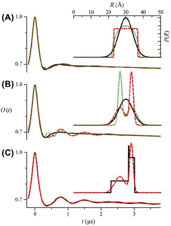
Calculated O(t) for the different P(R) shown in the insets. (A) O(t) for a unimodal Gaussian (black solid line), square (red dashed line), and circular (green dotted line) distributions. In all cases, r0 = 30 Å and σ = 4 Å. (B) O(t) for a unimodal Gaussian (black solid line) and bimodal Gaussian (r0−1 = 26.7 Å, σ1 = 3 Å, r0−2 = 33.3 Å, σ1 = 1 Å, f2 = 0.5, red dashed line; r0−1 = 26.7 Å, σ1 = 1 Å, r0−2 = 33.3 Å, σ1 = 3 Å, f2 = 0.5, green dotted line) distributions. In all cases 〈R〉 = 30 Å and σR = 4 Å. (C) O(t) for two bimodal distributions with either square (black solid line) or Gaussian components (red dashed line) (r0–1 = 26.7 Å, σ1 = 3 Å, r0–2 = 33.3 Å, σ1 = 1 Å, and f2 = 0.5).
3.2. Background signal
The background signal can be fit as an exponential or stretched exponential as defined in the following equation:
| (13) |
with
| (14) |
where d = 3 for an ideal 3-dimensional homogeneous solution. Using this approach to treat the background component of the DEER signal, the unknown parameter is λ for fixed d.
Alternatively a background signal can be calculated assuming a solution of singly-labeled spheres of radius ρ at concentration Ω. To calculate the background signal, a model is created with a single spin at the origin. A series of shells of increasing radius, q, is generated each containing an additional spin. Assuming that each of these spins is at the center of a spherical object, the distance of closest approach between spins is q0 = 2ρ. At a concentration of Ω (mM), an average of one spin will be contained in a volume ζ = (Ω × 6.022 × 10⁻¹⁰)−1 (Å3). Defining
| (15) |
and υk = υk−1 + ζ, then
| (16) |
and
| (17) |
is the width of the kth shell out to a maximum radius of qmax (typically 500 or 1000 Å).
The calculated background signal is given by the product of the modulations produced from all of the shells [10].
| (18) |
If the width of the shell is greater than an upper limit, ε′, it is necessary to perform additional averaging to calculate bk(t). Following Eq. (6), for εk > ε′
| (19) |
where
| (20) |
for all integers l ≥ 1 such that . For εk ≤ ε′ no additional averaging is necessary and
| (21) |
Fig. 2 shows background signals, B(t), calculated for different values of Ω and ρ using ΔB = 0.3. For ρ = 0 Å, B(t) is a product of modulations at all frequencies and the result correspond closely to an exponential decay, B(t) ∝ e−αt. Based on additional calculations (not shown), in the limit that ΔB → 0 for constant values of ΔB × Ω, the exponential decay rate approaches the theoretical value [29] of
| (22) |
Fig. 2.
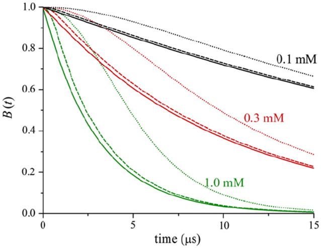
Calculated B(t) for different values of Ω and ρ. Ω = 0.1 mM (black lines), Ω = 0.3 mM (red lines), Ω = 1.0 mM (green lines). ρ = 0 Å (solid lines), ρ = 25 Å (dashed lines), ρ = 50 Å (dotted lines). In all cases ΔB = 0.3.
For ρ > 0 Å, B(t) deviates significantly from pure exponential behavior due to the loss of contributions at high frequencies as a result of the excluded volume effect.
Using B(t) to model the background signal, the unknown parameters are the modulation depth for the background signal, ΔB, together with Ω and ρ. In the absence of orientation selection effects, the factors determining Δ and ΔB are identical and these parameters can be linked in the analysis.
3.3. Preprocessing
Initially, the DEER data is phase-corrected by finding the phase that minimizes the sum of squared differences between the imaginary component and an unknown constant which should be near zero in the absence of certain hardware issues. This minimum sum of squared differences is subsequently used to estimate the noise level in the real component.
The experimental DEER signal, V′(t′), is measured to an arbitrary scale factor. Furthermore the true maximum value of the real component of V′ may be shifted from t′ = 0. Taking advantage of the symmetry of the DEER signal about t = 0 [9], V′(t′) at small values of |t′| is fit directly to a Gaussian function.
| (23) |
The scaled and time-shifted data is then given by
| (24) |
such that V(t) is now maximal at t ≈ 0 with V(0) ≈ 1 and V(t) can be fit using Eq. (3). Since the data for small |t′| is most sensitive to P(R), all of the data including that for t < 0 is included in the fit.
3.4. Fitting
For the global analysis of multiple data sets, the goal is to minimize the value of χ2 given by Eq. (25) [31]
| (25) |
where M is the total number of experimental data sets that are being fit, Nm is the number of experimental data points in the mth data set, δm is the estimated noise level in the mth data set, and Q is the total number of parameters being varied in the fit. The Marquardt–Levenberg (M–L) algorithm as previously implemented by Beechem [31] is used to search for the global χ2 minimum. In particular, the numerical derivative of the fitting function, F(t), with respect to a fit parameter is determined using an increment that is 0.1–1% of the parameter value. Using this approach resulted in consistently better fits than those obtained using the M–L algorithm as implemented in the MATLAB function “lsqcurvefit”.
Let be the value of χ2 found in the initial search using the M–L algorithm and let be the set of best-fit parameters. The values of and the corresponding parameters will, of course, depend on the initial values of the same parameters, . The question is whether corresponds to the true global χ2 minimum. Despite the inherent difficulty of fitting of DEER data, particularly without the use of a priori background correction, the approach outlined above has worked reliably to fit data using a model of a unimodal distance distribution and an exponential background decay. This model can be used as a starting point for subsequent fitting with more complex models, including multimodal distance distributions or backgrounds calculated with excluded volume effects. Using more complex models, there is a higher likelihood of encountering local minima in the χ2 surface. As outlined below, the calculation of confidence intervals provides an important tool for performing additional exploration of the χ2 surface in search of the true global χ2 minimum.
3.5. Confidence intervals
The primary purpose of the determination of confidence intervals is to determine how well-defined the parameter values are. Rather than relying on estimates of the parameter uncertainty based on the shape of the χ2 surface at , confidence intervals are explicitly determined through a series of additional M–L minimizations for each of the Q parameters [31,32]. To calculate the confidence interval for the qth of the Q fitting parameters, the value of that parameter is fixed to a series of values within a defined range. For each particular value of the qth parameter, the M–L algorithm is used to find the values of the Q − 1 other parameters that minimize χ2. An added benefit of this approach is that if is not the true global χ2 minimum, the calculation of confidence intervals will typically reveal a better fit. During the calculation of the confidence intervals for the Q fit parameters, the overall best-fit value of χ2 and the corresponding parameters are stored. If the best value of χ2 found in the confidence intervals is significantly lower than , then the best set of parameters found in the confidence intervals can be used as the starting point for a second round of fitting. This iterative approach, though time-consuming, has reliably identified what appears to be the true global χ2 minimum for all of the data considered to date.
During the calculation of the confidence interval for the qth parameter for each value of q examined, the best-fit values of χ2 and the other Q − 1 parameters are stored. Examination of the values of the other parameters as the value of q changes can reveal important correlations between parameters. Plots of the values of χ2 versus the values of the qth parameter indicate how precise the parameter values are. Strictly speaking, a confidence interval for a particular parameter is not the same as the uncertainty in that parameter. Nonetheless, qualitatively a relatively flat confidence interval suggests that the parameter is not well-determined and has a large uncertainty, while a steep confidence interval suggests the opposite. Quantitatively, the F-statistic can be used to determine the statistically significant increase in χ2 above at a given confidence level and confidence intervals reveal the parameter values that fall below this confidence level.
3.6. DeerAnalysis
For comparison, some data were also analyzed using the 2011 version of DeerAnalysis software (http://www.epr.ethz.ch/software/index) [9]. Unless otherwise noted, DeerAnalysis was run using default values. When fitting data to a model, the fits were repeatedly run until it appeared that convergence was achieved. When using Tikhonov regularization, the regularization parameter was chosen near the elbow of the L curve favoring values which gave better fits as opposed to smoother distributions.
4. Results and discussion
4.1. T4L
Fig. 3 shows the analysis of DEER data from T4L labeled at residues 65 and 80 (T4L 65/80). The best-fit parameters are given in Table 1. As shown in Fig. 3A, an excellent fit to the data was obtained assuming an exponential background (β = 1; dashed line) and a unimodal Gaussian distance distribution (inset). Fig. 3B shows the data and the fit with the background decay divided out of both and Fig. 3C shows the residuals for the fit. As expected, an equivalent fit (not shown) was obtained for a calculated background signal with a Ω = 0.20 mM and ρ fixed to a value of 0 Å (Table 1). No significant improvement in the fit was obtained for larger values of ρ. Fig. 3D shows confidence intervals for the parameters r0 and σ. From these confidence plots, values of r0 = 26.2 ± 0.5 Å and σ = 3.4 ± 0.8 Å fall below the 95% confidence level.
Fig. 3.
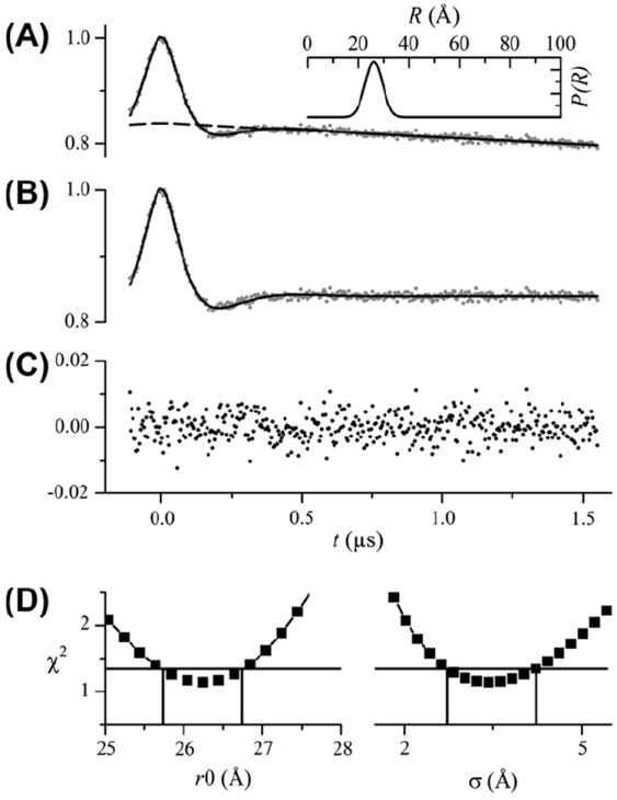
Analysis of DEER data from T4L 65/80. (A) DEER data after phasing and scaling is shown as gray dots. The best fit to the data using a single Gaussian distance distribution is shown as a solid line. The best-fit parameters are given in Table 1. The exponential background signal is shown as a dashed line. The inset shows the distance distribution. (B) The DEER data (gray dots) and fit (solid line) shown with the background exponential removed after the fit. (C) The residuals (data-fit) shown as black dots. (D) Confidence intervals plotted for the center (r0) and width (σ) of the distance distribution. The horizontal solid lines show the χ2 value corresponding to the 95% confidence level. The vertical lines indicate the range of parameter values within the 95% confidence interval.
Table 1.
Parameters from the analysis of DEER data from T4L labeled at residues 65/80 shown in Fig. 3.
| Δ | λ | Ω (mM) | ρ (Å) | r0 (Å) | σ (Å) | χ2 | |
|---|---|---|---|---|---|---|---|
| Fig. 3 | 0.16 | 4.52 | – | – | 26.2 | 3.4 | 1.14 |
| Not shown | 0.16 | – | 0.20 | 0a | 26.2 | 3.4 | 1.14 |
The value of ρ was fixed to 0 Å. A very small and statistically insignificant decrease in χ2 was obtained for a best-fit value of ρ = 15 Å.
The confidence intervals in Fig. 3D are searches through the χ2 surface along a single dimension. Alternatively Fig. 4 shows a multidimensional exploration of the χ2 surface similar to that used by Fajer and coworkers [4], performed by randomly selecting values of r0 and σ then optimizing Δ and λ to minimize χ2. It is clear that the confidence intervals (open black circles) are equivalent to the results of a multidimensional search (filled color circles) when the latter are projected onto the r0−χ2 and σ−χ2 planes. The disadvantage of the multidimensional approach is that considerably more distinct optimizations are required (252 = 625 versus 2 × 25 = 50 for the two confidence intervals). On the other hand, the multidimensional approach can reveal details about the shapes of the confidence levels.
Fig. 4.

Two-dimensional exploration of the χ2 surface for the fit in Fig. 3. For each point, random values of r0 and σ were selected then the other parameters varied to minimize χ2. For clarity, only the points (filled color circles) projected on the r0–χ2, σ–χ2, and r0–σ planes are shown. Points within the 95% confidence level are shown in red and those within the 67% confidence level are shown in green. Confidence intervals equivalent to those shown in Fig. 3D are plotted on the r0-χ2 and σ–χ2 planes (black lines and open circles).
For this particular data set, a distance distribution that is essentially identical to that obtained in Fig. 3 can be obtained fitting background corrected data using DeerAnalysis [9] and either a Gaussian distance distribution model or the Tikhonov regularization option (results not show). In addition, the Gaussian plus homogenous background model within DeerAnalysis also gives nearly identical results fitting the uncorrected data (results not show). The fact that GLADD and the various approaches within DeerAnalysis all successfully fit this data set and give nearly the same distance distribution is a direct result of the relatively short mean and narrow width of P(R) together with the relative long tmax value.
4.2. Simulated data
To directly compare the capabilities of GLADD and DeerAnalysis under more challenging conditions, both programs were used to fit simulated data sets. Data was simulated for a broad Gaussian distribution (Fig. 5A) and a bimodal Gaussian distribution (Fig. 7A) with an exponential background at four different values of tmax = 0.7, 1.4, 2.1, and 2.8 μs. The simulated data were analyzed using four different approaches.
Fig. 5.
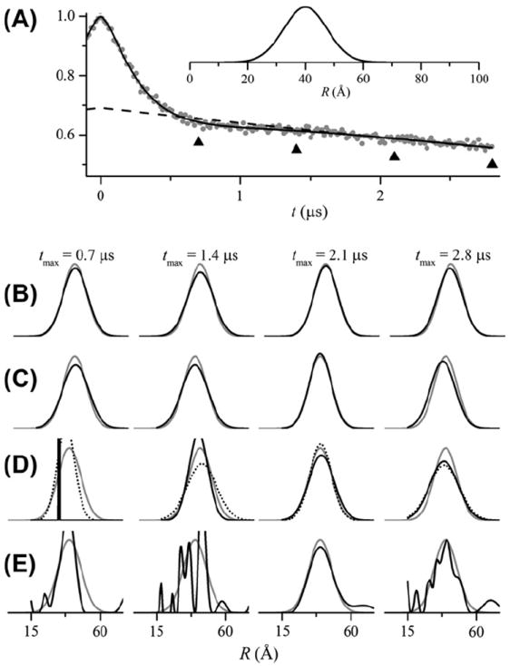
Analysis of simulated DEER signals for a broad unimodal Gaussian distance distribution using GLADD and DeerAnalysis. DEER signals were simulated for time values from t = −0.096 μs to tmax = 0.7, 1.4, 2.1, or 2.8 μs in time increments of 4, 8, 12, or 16 ns. A Gaussian distance distribution with r0 = 40 Å and σ = 7.5 Å was used. Exponential background decays were included using λ = 4.9 and β = 3 which corresponds to a spin concentration of approximately 240 μM. Random normal numbers were added to give a signal-to-noise ratio of 100:1. (A) The simulated data for tmax= 2.8 μs is shown (gray dots) together with the fit (solid black line) obtained from GLADD using a unimodal Gaussian distance distribution and an exponential background. The best-fit background component is shown as a dashed black line. The four different tmax values are indicated by upward pointing triangles. (B) Distance distributions obtained from GLADD for the four different tmax values (increasing from left to right) are shown as solid black lines. Here and in subsequent panels, the actual P(R) used to simulate the DEER signal is shown as a solid gray line. (C) Distance distributions (solid black lines) obtained from DeerAnalysis using the Gaussian with 3-D homogeneous background model and no a priori background correction. D) Distance distributions obtained from DeerAnalysis using the Gaussian model. Background correction was performed with a 3-D homogeneous background fitting to either the final 75% (results shown as solid black lines) or final 25% (dotted black lines) of the DEER signal at positive time. (E) Distance distributions (solid black lines) obtained from DeerAnalysis using Tikhonov regularization. Background correction was performed with a 3-D homogeneous background fitting. In each case, the time range for background correction was chosen using the validation tool within DeerAnalysis. All P(R) are plotted to the same scale. In some cases, narrow components are clipped. To allow for a direct comparison between the two programs, the initial values used for GLADD (panel B) were chosen such that the initial distance distribution was the same as that used in DeerAnalysis (panel C) and other parameters (i.e. Δ and λ) were chosen to closely match the corresponding values in DeerAnalysis.
Fig. 7.
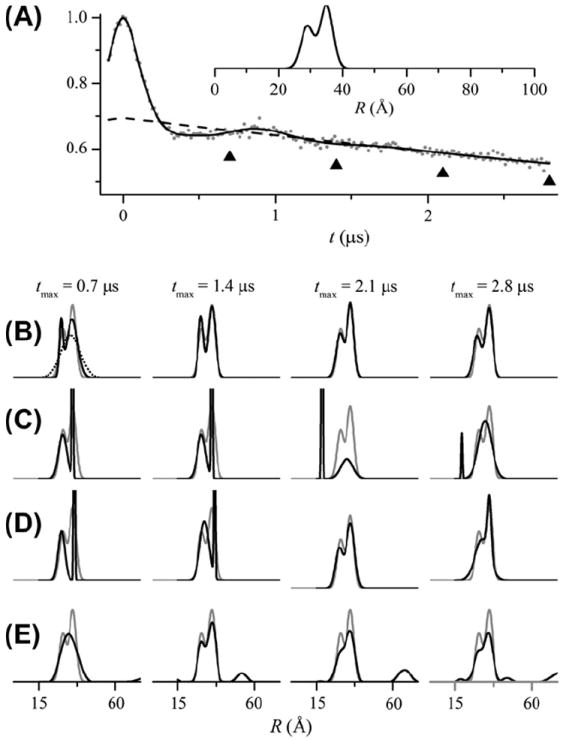
Analysis of simulated DEER signals for a bimodal Gaussian distance distribution using GLADD and DeerAnalysis. DEER signals were simulated as in Fig. 5 with r0_1 = 29 Å, σ1 = 2 Å, r0_2 = 35 Å, σ2 = 2 Å, and f2 = 0.6. (A) The simulated data for tmax = 2.8 μs is shown (gray dots) together with the fit (solid black line) obtained from GLADD using a bimodal Gaussian distance distribution and an exponential background. The best-fit background component is shown as a dashed black line. The four different tmax values are indicated by upward pointing triangles. (B) Distance distributions obtained from GLADD for the four different tmax values (increasing from left to right) are shown as black lines. Here and in subsequent panels, the actual P(R) used to simulate the DEER signal is shown as a solid gray line. The results from an initial fit to the tmax = 0.7 μs data is shown as a dotted line. In this case, the determination of confidence intervals revealed a better fit (solid line). (C) Distance distributions (solid black lines) obtained from DeerAnalysis using the two Gaussians with 3-D homogeneous background model and no a priori background correction. (D) Distance distributions (solid black lines) obtained from DeerAnalysis using the two Gaussian model. Initial background correction was performed with a 3-D homogeneous background fitting to the final 25% of the DEER signal at positive time. (E) Distance distributions (solid black lines) obtained from DeerAnalysis using Tikhonov regularization. Background correction was performed with a 3-D homogeneous background fitting. In each case, the time range for background correction was chosen using the validation tool within DeerAnalysis. All P(R) are plotted to the same scale. In some cases, narrow components are clipped. To allow for a direct comparison between the two programs, the initial values used for GLADD (panel B) were chosen such that the initial distance distribution was the same as that used in DeerAnalysis (panel C) and other parameters (i.e. Δ and λ) were chosen to closely match the corresponding values in DeerAnalysis.
GLADD using either a unimodal (Fig. 5B) or bimodal (Fig. 7B) Gaussian distance distribution with an exponential background.
DeerAnalysis with no background correction and either the Gaussian plus homogeneous background model (Fig. 5C) or the two Gaussian (Fig. 7C) plus homogeneous background model.
DeerAnalysis using a priori exponential background correction and either a Gaussian (Fig. 5D) or two Gaussian (Fig. 7D) distance distribution.
DeerAnalysis using a priori exponential background correction together with Tikhonov regularization, L curve computation, and the validation tool (Figs. 5E and 7E).
Fig. 5B shows the P(R) obtained (black lines) from fitting the simulated data using GLADD at four different tmax values. For all four tmax values, the P(R) obtained reasonably match the true distribution (gray lines). Fig. 6A shows the confidence intervals for the λ parameter for these same four fits. For the two smallest tmax values there is no lower limit on the range of values that fall below the 95% (dashed line) or even the 66% (dotted line) confidence levels. Fitting the data with a flat background (α = 0) cannot be ruled out. Thus, the background cannot be unambiguously resolved at the smaller tmax values and caution is warranted in interpreting these results. Fig. 6B through E show how the best-fit distance distributions correlate to the value of λ over the range that falls within the 95% confidence level. Clearly, there is a reduction in the variation in P(R) for λ values within the 95% confidence level at longer tmax values.
Fig. 6.

(A) Confidence intervals for λ from the fits using GLADD to the simulated data in Fig. 5 for tmax = 0.7 μs (open black squares), tmax = 1.4 μs (closed red circles), tmax = 2.1 μs (open green triangles), and tmax = 2.8 μs (closed blue diamonds). The horizontal dashed blue line shows the 95% confidence level for the tmax = 2.8 μs results. (B–E) The best-fit distance distributions at the λ values indicated by the open circles in panel A for tmax = 0.7 μs (B), tmax = 1.4 μs (C), tmax = 2.1 μs (D), and tmax = 2.8 μs (E) shown as dashed purple lines (low λ values) and dotted navy blue lines (high λ values) together with the actual distance distribution used to simulate the DEER data (solid gray lines). For tmax = 0.7 μs and tmax = 1.4 μs, the lower λ value (off-scale in panel A) was chosen at a point at which P(R) no longer changed. All P(R) are plotted to the same scale. In panel B, a narrow distribution is clipped.
Fig. 5C shows the P(R) (black lines) obtained from fitting the same simulated DEER data using the Gaussian plus homogeneous background model within DeerAnalysis. Again, for all four tmax values, the P(R) obtained reasonably match the true distribution (gray lines). Using either GLADD or DeerAnalysis, the simulated data in Fig. 5 can be successfully analyzed without a priori background correction.
Fig. 5D shows the P(R) obtained within DeerAnalysis using a priori exponential background correction and a Gaussian distance distribution with two different ranges of the data used for background fitting. Finally, Fig. 5E shows the P(R) obtained using a priori exponential background correction and Tikhonov regularization to obtain a model-free representation of the distribution. Depending on the range of data used for background fitting and the regularization parameter in the case of Tikhonov regularization, there is significant variation in P(R) when using a priori exponential background correction.
Fig. 7 shows corresponding results for simulated data for a bimodal Gaussian distribution. Fig. 7B and C shows the P(R) obtained from fitting the simulated data without background correction using GLADD and DeerAnalysis respectively. It is noteworthy that the initial fit from GLADD to the simulated data for tmax = 0.7 μs gave a broad unimodal-like distribution (dotted line). However, during the calculation of the confidence intervals for this fit a much better fit was revealed whose P(R) (solid black line) more closely matched the true bimodal distribution (solid gray line). Also noteworthy is that DeerAnalysis did not give the correct distribution for the tmax = 2.1 or 2.8 μs data using the two Gaussians plus homogeneous background model (Fig. 7C). Adjusting the initial parameters within DeerAnalysis to more closely match the true distribution parameters did give a better fit with a lower r.m.s. error to the data and a P(R) that more closely matched the true distribution. However, this adjustment had to be performed manually and, in this case, with knowledge of the true distance distribution. Fig. 7D and E show the P(R) obtained using a priori exponential background correction within DeerAnalysis using either a two Gaussian distance distribution or Tikhonov regularization, respectively.
The results in Figs. 5-7 suggest that GLADD can be used to analyze DEER data without a priori background correction. While the results in Fig. 6A–C demonstrate that, for short tmax, the λ value that determines the decay rate of the background exponential may not be defined at the low end, the confidence interval calculations can be used to define the resulting uncertainty in P(R). In the case of the bimodal distance distribution and the shortest tmax value, the initial fit using GLADD failed to reach the global χ2 minimum. However, the confidence interval calculations did reveal a much better fit to the data. Arguably, GLADD does a better job than DeerAnalysis of reproducing the true P(R) for the bimodal distribution at all tmax values (Fig. 7B versus C) when fitting data without a priori background correction.
Given this result and the warnings about fitting data without a priori background correction, it is important to consider what are the practical differences between GLADD and DeerAnalysis. Apart from differences in how data is preprocessed, the major differences between the two programs are the algorithms used for non-linear least-squares optimization and the approach used for error analysis. GLADD uses a version of the M–L algorithm while DeerAnalysis uses the Nelder–Mead (N–M) simplex algorithm as implemented in the MATLAB routine “fminsearch”. During the development of GLADD unsuccessful attempts were made to use the intrinsic optimization routines in MATLAB “fminsearch” (N–M) and “lsqcurvefit” (M–L). In short, there are issues with the scaling of the unknown variables in the MATLAB routines that do not exist in the “homemade” version of the M–L algorithm used in GLADD. Also, as discussed in the preceding paragraph, the calculation of confidence intervals is an important advantage in the event that GLADD initially becomes trapped in a local minimum.
4.3. CDB3
Fig. 8A shows a fit of DEER data from the CDB3 dimer spin-labeled at residue 340 with an exponential background and a single Gaussian distance distribution using GLADD. As is evident, a good fit to the data could not be obtained. On the other hand, a dramatic improvement in the fit was obtained for a calculated background signal including the excluded volume effect with a best-fit value of ρ = 33.5 Å (Fig. 8C and Table 2). The confidence intervals for the parameters Ω, ρ, r0, and σ shown in Fig. 9 demonstrate that all of these parameters are well-defined.
Fig. 8.
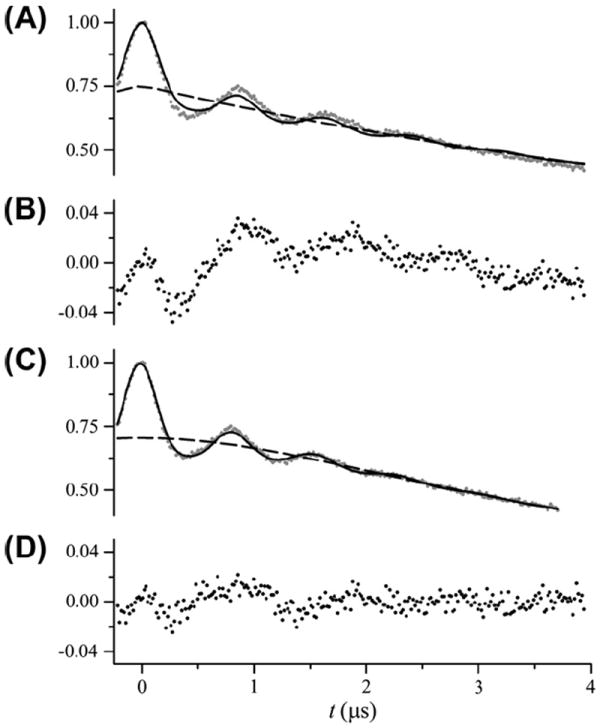
Analysis of DEER data from the CDB3 homodimer spin labeled at residue 340. (A) Fit (solid line) to the data (gray dots) using an exponential background (dashed line) and a single Gaussian distance distribution. (B) Residuals for the fit in (A). (C) Fit (solid line) to the data (gray dots) using a calculated background (dashed line) including an excluded volume effect and a single Gaussian distance distribution. (D) Residuals for the fit in C. The best-fit parameters are given in Table 2.
Table 2.
Parameters from the analyses of DEER data from CDB3 labeled at residue 340 shown in Fig. 8
Fig. 9.
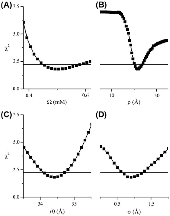
Selected confidence intervals for parameters from the fit in Fig. 8. The horizontal solid lines show the χ2 value corresponding to the 95% confidence level.
The background signal used in Fig. 8C (dashed line) was calculated for a model of a solution of singly-labeled spheres, Ω = 0.5 mM, of radius of ρ = 34 Å with the assumption that the spins are at the center of the spheres, while the experimental sample is a solution of doubly-labeled non-spherical protein dimers with spins closer to the surface. Nonetheless, the value of Ω agrees roughly with the actual spin concentration of 0.3 mM. Also, in contrast to the much smaller T4L (18.6 kD), the larger CDB3 dimer (85 kD) required a non-zero value of ρ to fit the data.
The value of ρ = 34 Å is in reasonable agreement with the dimensions of the CDB3 dimer observed in X-ray crystallography studies, approximately 75 × 55 × 45 Å [33], and with the measured values of its Stokes radius, 53 Å, at physiological pH [34]. Nonetheless not all of the sites on CDB3 used to measure the intra-dimer distance exhibited background signals with such a strong excluded volume effect. The extent to which a non-zero value of ρ was required to give a good fit to the data depended on a number of different factors including the tmax and the distance distribution. At site 340, the large difference between the values of χ2 obtained for ρ = 0 Å and that obtained for the optimal ρ are due to the long tmax used and to the narrow distance distribution.
The DEER data from CDB3 340 were collected with a sufficiently long tmax that, if the background were truly exponential, a clean background correction should be possible. Nevertheless a poor fit was obtained regardless of whether methods requiring a priori background correction (results not shown) or a fit including an exponential background (Fig. 8A) were used. While the model used for generating the background signal does not correspond strictly to the actual experimental sample, the result in Fig. 8C indicates that this model does have sufficient power to model the excluded volume effect evident in the data and to dramatically improve the fit.
While in many cases experimental background signals can be measured on singly labeled samples, in the case of the CDB3 dimer it is not possible to create singly-labeled samples at the appropriate protein and spin concentrations. Thus, the use of an experimentally determined background for background correction is not possible in this case. Data collected from samples of the CDB3 dimer labeled at residue 340 with a mixture of paramagnetic and non-paramagnetic methanethiosulfonates demonstrate the same non-exponential background signal but also show the modulation of the specific interaction though at a reduced modulation depth (see Supplementary data).
In summary, DEER data collected from certain sites in the CDB3 dimer could not be properly fit using a priori background correction with either an exponential function or an experimentally determined signal. At these sites, the fit to the data was dramatically improved by using a background calculated for a model including an excluded volume effect. The parameters obtained from these fits are reasonable given the overall size of the CDB3 dimer. In this case the inclusion of the excluded volume effect does not have a large effect on the P(R) obtained from the analysis. Nonetheless, the errors in the fit shown in Fig. 8A are as large as or larger than the changes in the DEER signal caused by the biologically relevant mutation discussed in the next section. Consequently, it was important to start with the best possible fit to this data.
4.4. P327R Cdb3
Previous work has shown that a proline to arginine mutation at residue 327 in CDB3 affects the packing of the C-terminal end of helix 10 of the dimerization arms in a subpopulation of CDB3 dimers [28]. The result is a second component in the distance distribution observed in DEER data from selected sites within the dimerization arms. Fig. 10A shows a fit of the DEER data from CDB3 spin labeled at residue 340, the same data as in Fig. 8, assuming a bimodal Gaussian distribution. The best-fit parameters are given in Table 3. The bimodal Gaussian distance distribution gives only a slight improvement in χ2 over a single Gaussian (1.70 versus 1.80). On the other hand, the fit to the data from P327R CDB3 spin labeled at residue 340 is significantly improved using a bimodal Gaussian distribution (χ2 = 1.35 versus χ2 = 2.19).
Fig. 10.
Analysis of DEER data from P327 and P327R CDB3 homodimers spin labeled at residue 340. (A) Fit to the data from P327 CDB3 340 (same data as Fig. 8) using a calculated background including an excluded volume effect and a bimodal Gaussian distance distribution. The data (gray dots) and fit (solid black line) are shown with the background removed after the fit. (B) Fit to the data from P327R CDB3 340 using a calculated background including an excluded volume effect and a bimodal Gaussian distance distribution. The data (gray dots) and fit (solid black line) are shown with the background removed after the fit. (C) The bimodal Gaussian distance distributions from the fits to the P327 (solid line) and P327R (dashed line) data. The best-fit parameters are given in Table 3.
Table 3.
Parameters from the analyses of DEER data from P327 and P327R CDB3 labeled at residue 340 shown in Fig. 10.
The proline to arginine mutation at residue 327 in CDB3 causes a clinically relevant hereditary spherocytosis [35] and it had been suggested that this mutation could disrupt dimerization [33]. Previous results [28] and the results presented here demonstrate that the P327R mutant of CDB3 does fully dimerize. In particular, both P327 and P327R CDB3 labeled at residue 340 give DEER modulations depths of 0.29–0.30 (Table 3) indicating both are fully dimerized. The results in Fig. 11 give important insights into the subtle structural changes assoctiated with the P327R mutation. The confidence interval for f2 is quite flat for P327 CDB3 and the χ2 value for f2 = 0 does fall below the 95% confidence level. On the other hand, for the P327R CDB3 mutant the addition of a second component to the distance distribution does significantly improve χ2 for the data from site 340 and similar results have been obtained at other sites in the dimerization arms. In addition, the confidence intervals for r0_1 (Fig. 11B) indicate that the small, 0.5 Å, shift measured in the center of the major component is significant, that it does reflect a true consequence of the P327R mutation, and that it is not an artifact.
Fig. 11.
Selected confidence intervals for parameters from the fits in Fig. 10. The solid squares are from the fits to the P327 data; open circles are from the fits to the P327R data. The horizontal solid lines show the χ2 value corresponding to the 95% confidence level. All χ2 values have been adjusted so that the best-fit gives χ2 = 1.
4.5. Global analysis
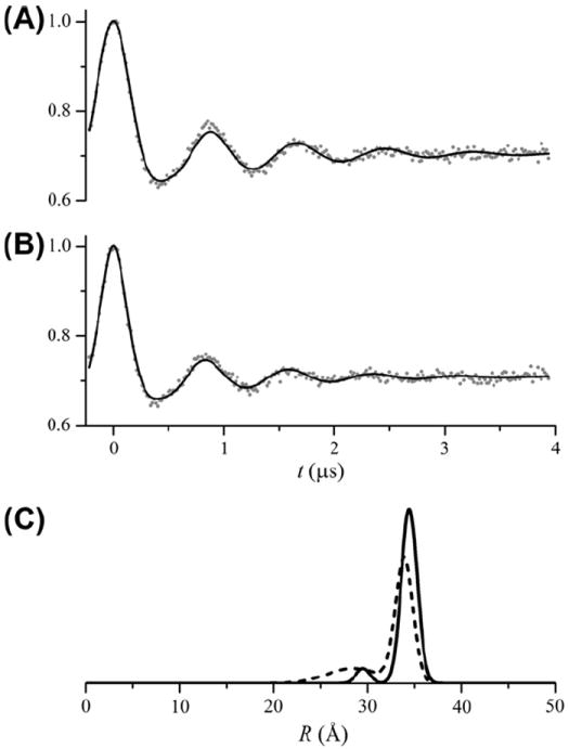
In typical site-directed spin labeling experiments the MTSSL label exhibits considerable flexibility with respect to the protein. On the other hand, the CW-EPR spectrum of the CDB3 dimer spin-labeled at residue 290 is near the rigid limit as is consistent with a nitroxide in an environment with a large degree of steric hindrance. Likewise, the DEER data from this same site shows a highly persistent modulation pattern characteristic of a very narrow distance distribution [11]. These results prompted further DEER measurements to test whether DEER data varies systematically as a function of the frequency separation between the observe and pump pulses, Δν, which would be indicative of orientation selection. Small orientation selection effects are, in fact, present in the data collected at the three different Δν in Fig. 12A. These effects manifest as variations in the relative amplitudes of two different components whose frequencies differ by approximately a factor of two [36]. These two frequencies correspond to the two turning points in the Pake pattern corresponding to θ = 0° and 90° (Eq. (5)). Variations in their relative amplitudes are due to deviations from the ideal Pake pattern that would be observed in the absence of orientation effects.
Fig. 12.
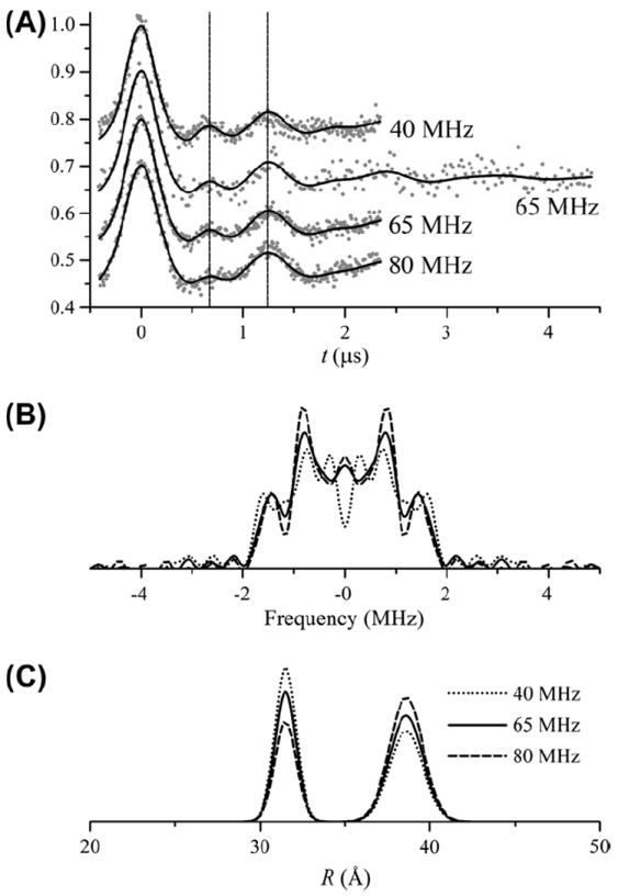
Global analysis of DEER data from the CDB3 homodimer spin labeled at residue 290. (A) DEER data (gray dots) collected at three different separations between observe and pump pulse frequencies as indicated (Δν = 40, 65, and 80 MHz). Data at 65 MHz were collected for two different values of tmax. The modulation curves show two different components whose frequencies differ by approximately a factor of two. Dashed lines indicate the first crests of the two frequency components. The global analysis was performed with a bimodal Gaussian distance distribution with parameters given in Table 4. All of the data and fits are shown with the background removed after the analysis. The best-fit parameters are given in Table 4. (B) Fourier transforms of the data in A. (C) The best-fit distance distributions for the three different frequency separations.
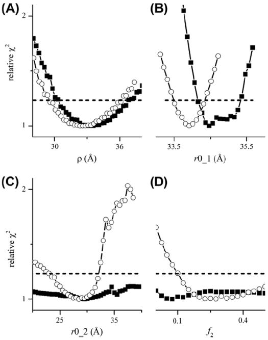
In an initial attempt to fit the data in Fig. 12, a bimodal Gaussian distance distribution was used with the values of Ω, ρ, r0, and σ linked between all of the data sets. Selective confidence intervals for this fit are shown in Fig. 13. Only the modulation depths, Δ, and the relative amplitudes of the two components were allowed to vary at the different frequency separations (Table 4).
Fig. 13.
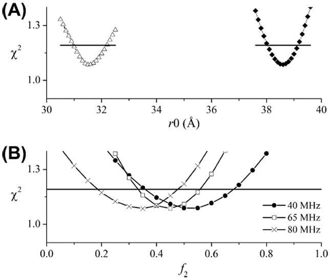
Confidence intervals for the fits in Fig. 12. (A) Confidence intervals for r0_1 (closed diamonds) and r0_2 (open triangles). (B) Confidence intervals for the relative amplitudes of the second component, f2, at the three different frequency separations as indicated. The horizontal dashed lines show the 95% confidence level.
Table 4.
Parameters from the analysis of DEER data from CDB3 labeled at residue 290 shown in Fig. 12
| Δν (MHz) | Δ | Ω (mM) | ρ (Å) | r0_1 (Å) | σ1 (Å) | r0_2 (Å) | σ2 (Å) | f2 |
|---|---|---|---|---|---|---|---|---|
| 40 | 0.21 | 0.480 | 30 | 38.6 | 1.0 | 31.5 | 0.6 | 0.52 |
| 65 | 0.23 | Linked | Linked | Linked | Linked | Linked | Linked | 0.44 |
| 80 | 0.22 | Linked | Linked | Linked | Linked | Linked | Linked | 0.34 |
Algorithms have been developed for rigorously including orientation effects in the modeling of DEER data [37-41] and in some cases data obtained at multiple pump–probe frequency separations has been simultaneously fit to determine orientation parameters [24-26]. Here, all of the data in Fig. 12A were globally analyzed using a much simpler model. No attempt has been made, at this point, to properly include the relative orientation of the two labels in the model. Instead, the approach used here is an ad hoc demonstration of the potential utility of global analysis in the fitting of DEER data. As outlined in the Introduction, there are a number of experimental situations where multiple DEER data sets could be collected and combined into a single analysis. The flexibility of the approach developed here allows it to be adapted to all of these different circumstances.
5. Conclusions
The results presented here demonstrate that a priori background correction of DEER data is not required for routine fitting. When the object under study is of sufficient size, the background DEER signal can deviate significantly from exponential behavior due to an excluded volume effect. An algorithm has been developed for modeling this effect. In addition, the approach developed allows for a rigorous error analysis of the fitting parameters. Finally, the global analysis of multiple DEER data sets has been demonstrated laying the foundation for a number of important applications of this approach.
Supplementary Material
Acknowledgments
The authors wish to thank Dr. Bruce H. Robinson for his insights on global analysis and non-linear least squares algorithms. Drs. Richard A. Stein and Olav Schiemann participated in many helpful discussions on the fitting of DEER data and both commented on the manuscript prior to submission. Dr. Hassane S. Mchaourab generously provided the reagents for the T4L sample. This work was supported by the National Institutes of Health through P01 GM080513.
Footnotes
Appendix A. Supplementary material
Supplementary data associated with this article can be found, in the online version, at http://dx.doi.org/10.1016/j.jmr.2012.03.006.
References
- 1.Pannier M, Veit S, Godt A, Jeschke G, Spiess HW. Dead-time free measurement of dipole–dipole interactions between electron spins. J Magn Reson. 2000;142:331–340. doi: 10.1006/jmre.1999.1944. [DOI] [PubMed] [Google Scholar]
- 2.Reginsson GW, Schiemann O. Pulsed electron–electron double resonance: beyond nanometre distance measurements on biomacromolecules. Biochem J. 2011;434:353–363. doi: 10.1042/BJ20101871. [DOI] [PubMed] [Google Scholar]
- 3.Reginsson GW, Schiemann O. Studying bimolecular complexes with pulsed electron–electron double resonance spectroscopy. Biochem Soc Trans. 2011;39:128–139. doi: 10.1042/BST0390128. [DOI] [PubMed] [Google Scholar]
- 4.Fajer PG, Brown L, Song L. Kluwer Academic/Plenum Publ. Vol. 233. Spring St.; New York, NY, USA: 2007. Practical Pulsed Dipolar ESR (DEER) [Google Scholar]
- 5.Jeschke G, Pannier M, Godt A, Spiess HW. Dipolar spectroscopy and spin alignment in electron paramagnetic resonance. Chem Phys Lett. 2000;331:243–252. [Google Scholar]
- 6.Borbat PP, McHaourab HS, Freed JH. Protein structure determination using long-distance constraints from double-quantum coherence ESR: study of T4 lysozyme. J Am Chem Soc. 2002;124:5304–5314. doi: 10.1021/ja020040y. [DOI] [PubMed] [Google Scholar]
- 7.Bowman MK, Maryasov AG, Kim N, DeRose VJ. Visualization of distance distribution from pulsed double electron–electron resonance data. Appl Magn Reson. 2004;26:23–39. [Google Scholar]
- 8.Chiang YW, Borbat PP, Freed JH. The determination of pair distance distributions by pulsed ESR using Tikhonov regularization. J Magn Reson. 2005;172:279–295. doi: 10.1016/j.jmr.2004.10.012. [DOI] [PubMed] [Google Scholar]
- 9.Jeschke G, Chechik V, Ionita P, Godt A, Zimmermann H, Banham J, Timmel CR, Hilger D, Jung H. DeerAnalysis2006 – a comprehensive software package for analyzing pulsed ELDOR data. Appl Magn Reson. 2006;30:473–498. [Google Scholar]
- 10.Jeschke G, Koch A, Jonas U, Godt A. Direct conversion of EPR dipolar time evolution data to distance distributions. J Magn Reson. 2002;155:72–82. doi: 10.1006/jmre.2001.2498. [DOI] [PubMed] [Google Scholar]
- 11.Zhou Z, DeSensi SC, Stein RA, Brandon S, Dixit M, McArdle EJ, Warren EM, Kroh HK, Song LK, Cobb CE, Hustedt EJ, Beth AH. Solution structure of the cytoplasmic domain of erythrocyte membrane band 3 determined by site-directed spin labeling. Biochemistry. 2005;44:15115–15128. doi: 10.1021/bi050931t. [DOI] [PubMed] [Google Scholar]
- 12.Hilger D, Polyhach Y, Jung H, Jeschke G. Backbone structure of transmembrane domain IX of the Na(+)/proline transporter PutP of Escherichia coli. Biophys J. 2009;96:217–225. doi: 10.1016/j.bpj.2008.09.030. [DOI] [PMC free article] [PubMed] [Google Scholar]
- 13.Kim S, Brandon S, Zhou Z, Cobb CE, Edwards SJ, Moth CW, Parry CS, Smith JA, Lybrand TP, Hustedt EJ, Beth AH. Determination of structural models of the complex between the cytoplasmic domain of erythrocyte band 3 and ankyrin-R repeats 13–24. J Biol Chem. 2011;286:20746–20757. doi: 10.1074/jbc.M111.230326. [DOI] [PMC free article] [PubMed] [Google Scholar]
- 14.Hilger D, Polyhach Y, Padan E, Jung H, Jeschke G. High-resolution structure of a Na+/H+ antiporter dimer obtained by pulsed election paramagnetic resonance distance measurements. Biophys J. 2007;93:3675–3683. doi: 10.1529/biophysj.107.109769. [DOI] [PMC free article] [PubMed] [Google Scholar]
- 15.Park S-Y, Borbat PP, Gonzalez-Bonet G, Bhatnagar J, Pollard AM, Freed JH, Bilwes AM, Crane BR. Reconstruction of the chemotaxis receptor-kinase assembly. Nat Struct Mol Biol. 2006 doi: 10.1038/nsmb1085. [DOI] [PubMed] [Google Scholar]
- 16.Sen KI, Wu H, Backer JM, Gerfen GJ. The structure of p85ni in class IA phosphoinositide 3-kinase exhibits interdomain disorder. Biochemistry. 2010;49:2159–2166. doi: 10.1021/bi902171d. [DOI] [PMC free article] [PubMed] [Google Scholar]
- 17.Zou P, Bortolus M, Mchaourab HS. Conformational cycle of the ABC transporter MsbA in liposomes: detailed analysis using double electron–electron resonance spectroscopy. J Mol Biol. 2009;393:586–597. doi: 10.1016/j.jmb.2009.08.050. [DOI] [PMC free article] [PubMed] [Google Scholar]
- 18.Altenbach C, Kusnetzow AK, Ernst OP, Hofmann KP, Hubbell WL. High-resolution distance mapping in rhodopsin reveals the pattern of helix movement due to activation. Proc Natl Acad Sci USA. 2008;105:7439–7444. doi: 10.1073/pnas.0802515105. [DOI] [PMC free article] [PubMed] [Google Scholar]
- 19.Van Eps N, Preininger AM, Alexander N, Kaya AI, Meier S, Meiler J, Hamm HE, Hubbell WL. Interaction of a G protein with an activated receptor opens the interdomain interface in the alpha subunit. Proc Natl Acad Sci USA. 2011;108:9420–9424. doi: 10.1073/pnas.1105810108. [DOI] [PMC free article] [PubMed] [Google Scholar]
- 20.Blackburn ME, Veloro AM, Fanucci GE. Monitoring inhibitor-induced conformational population shifts in HIV-1 protease by pulsed EPR spectroscopy. Biochemistry. 2009;48:8765–8767. doi: 10.1021/bi901201q. [DOI] [PubMed] [Google Scholar]
- 21.Claxton DP, Quick M, Shi L, de Carvalho FD, Weinstein H, Javitch JA, Mchaourab HS. Ion/substrate-dependent conformational dynamics of a bacterial homolog of neurotransmitter: sodium symporters. Nat Struct Mol Biol. 2010;17:U822–U868. doi: 10.1038/nsmb.1854. [DOI] [PMC free article] [PubMed] [Google Scholar]
- 22.Grote M, Polyhach Y, Jeschke G, Steinhoff HJ, Schneider E, Bordignon E. Transmembrane signaling in the maltose ABC transporter MalFGK2-E: periplasmic MalF-P2 loop communicates substrate availability to the ATP-bound MalK dimer. J Biol Chem. 2009;284:17521–17526. doi: 10.1074/jbc.M109.006270. [DOI] [PMC free article] [PubMed] [Google Scholar]
- 23.Hustedt EJ, Smirnov AI, Laub CF, Cobb CE, Beth AH. Molecular distances from dipolar coupled spin-labels: the global analysis of multifrequency continuous wave electron paramagnetic resonance data. Biophys J. 1997;72:1861–1877. doi: 10.1016/S0006-3495(97)78832-5. [DOI] [PMC free article] [PubMed] [Google Scholar]
- 24.Denysenkov VP, Prisner TF, Stubbe J, Bennati M. High-field pulsed electron–electron double resonance spectroscopy to determine the orientation of the tyrosyl radicals in ribonucleotide reductase. Proc Natl Acad Sci USA. 2006;103:13386–13390. doi: 10.1073/pnas.0605851103. [DOI] [PMC free article] [PubMed] [Google Scholar]
- 25.Savitsky A, Dubinskii AA, Flores M, Lubitz W, Moebius K. Orientation-resolving pulsed electron dipolar high-field EPR spectroscopy on disordered solids: I. Structure of spin-correlated radical pairs in bacterial photosynthetic reaction centers. J Phys Chem B. 2007;111:6245–6262. doi: 10.1021/jp070016c. [DOI] [PubMed] [Google Scholar]
- 26.Yang Z, Kise D, Saxena S. An approach towards the measurement of nanometer range distances based on Cu(2+) ions and ESR. J Phys Chem B. 2010;114:6165–6174. doi: 10.1021/jp911637s. [DOI] [PubMed] [Google Scholar]
- 27.Hustedt EJ, Stein RA, Sethaphong L, Brandon S, Zhou Z, DeSensi SC. Dipolar coupling between nitroxide spin labels: the development and application of a tether-in-a-cone model. Biophys J. 2006;90:340–356. doi: 10.1529/biophysj.105.068544. [DOI] [PMC free article] [PubMed] [Google Scholar]
- 28.Zhou Z, DeSensi SC, Stein RA, Brandon S, Song L, Cobb CE, Hustedt EJ, Beth AH. Structure of the cytoplasmic domain of erythrocyte band 3 hereditary spherocytosis variant P327R: band 3 Tuscaloosa. Biochemistry. 2007;46:10248–10257. doi: 10.1021/bi700948p. [DOI] [PubMed] [Google Scholar]
- 29.Jeschke G, Panek G, Godt A, Bender A, Paulsen H. Data analysis procedures for pulse ELDOR measurements of broad distance distributions. Appl Magn Reson. 2004;26:223–244. [Google Scholar]
- 30.Milov AD, Maryasov AG, Tsvetkov YD. Pulsed electron double resonance (PELDOR) and its applications in free-radicals research. Appl Magn Reson. 1998;15:107–143. [Google Scholar]
- 31.Beechem JM. Global analysis of biochemical and biophysical data. Methods Enzymol. 1992;210:37–54. doi: 10.1016/0076-6879(92)10004-w. [DOI] [PubMed] [Google Scholar]
- 32.Johnson ML. Evaluation and propagation of confidence intervals in nonlinear, asymmetrical variance spaces. Analysis of ligand-binding data. Biophys J. 1983;44:101–106. doi: 10.1016/S0006-3495(83)84281-7. [DOI] [PMC free article] [PubMed] [Google Scholar]
- 33.Zhang DC, Kiyatkin A, Bolin JT, Low PS. Crystallographic structure and functional interpretation of the cytoplasmic domain of erythrocyte membrane band 3. Blood. 2000;96:2925–2933. [PubMed] [Google Scholar]
- 34.Appell KC, Low PS. Partial structural characterization of the cytoplasmic domain of the erythrocyte-membrane protein, band-3. J Biol Chem. 1981;256:1104–1111. [PubMed] [Google Scholar]
- 35.Jarolim P, Palek J, Rubin HL, Prchal JT, Korsgren C, Cohen CM. Band 3 Tuscaloosa: Pro327 -- Arg327 substitution in the cytoplasmic domain of erythrocyte band 3 protein associated with spherocytic hemolytic anemia and partial deficiency of protein 4.2. Blood. 1992;80:523–529. [PubMed] [Google Scholar]
- 36.Endeward B, Butterwick JA, MacKinnon R, Prisner TF. Pulsed electron–electron double-resonance determination of spin-label distances and orientations on the tetrameric potassium ion channel KcsA. J Am Chem Soc. 2009;131:15246–15250. doi: 10.1021/ja904808n. [DOI] [PMC free article] [PubMed] [Google Scholar]
- 37.Larsen RG, Singel DJ. Double electron–electron resonance spin-echo modulation: spectroscopic measurement of electron spin pair separations in orientationally disordered solids. J Chem Phys. 1993;98:5134–5146. [Google Scholar]
- 38.Margraf D, Bode BE, Marko A, Schiemann O, Prisner TF. Conformational flexibility of nitroxide biradicals determined by X-band PELDOR experiments. Mol Phys. 2007;105:2153–2160. [Google Scholar]
- 39.Marko A, Margraf D, Cekan P, Sigurdsson ST, Schiemann O, Prisner TF. Analytical method to determine the orientation of rigid spin labels in DNA. Phys Rev E. 2010;81 doi: 10.1103/PhysRevE.81.021911. [DOI] [PubMed] [Google Scholar]
- 40.Marko A, Margraf D, Yu H, Mu Y, Stock G, Prisner T. Molecular orientation studies by pulsed electron–electron double resonance experiments. J Chem Phys. 2009;130 doi: 10.1063/1.3073040. [DOI] [PubMed] [Google Scholar]
- 41.Polyhach Y, Godt A, Bauer C, Jeschke G. Spin pair geometry revealed by high-field DEER in the presence of conformational distributions. J Magn Reson. 2007;185:118–129. doi: 10.1016/j.jmr.2006.11.012. [DOI] [PubMed] [Google Scholar]
Associated Data
This section collects any data citations, data availability statements, or supplementary materials included in this article.