

Abstract
Quantitative models of development that consider all relevant genes typically are difficult to fit to embryonic data alone and have many redundant parameters. Computational evolution supplies models of phenotype with relatively few variables and parameters that allows the patterning dynamics to be reduced to a geometrical picture for how the state of a cell moves. The clock and wavefront model, that defines the phenotype of somitogenesis, can be represented as a sequence of two discrete dynamical transitions (bifurcations). The expression-time to space map for Hox genes and the posterior dominance rule are phenotypes that naturally follow from computational evolution without considering the genetics of Hox regulation.
Introduction
Classically, phenotype has been a description of states rather than the transitions between them. But development is inherently about change, and any comprehensive mathematical description will be dynamical and require knowledge of rate parameters as well as state parameters. There is a natural language for dynamics through geometry, already recognized by Waddington and his successors [1, 2], that provides a parsimonious and effective way to quantify phenotype. Geometry in this context implies that we describe the system by a few abstract variables that are indicative of phenotype, and parameterize them in such a way as to make the transitions in dynamical behavior, e.g., from stable to oscillating, as simple as possible. Dynamics is represented as field of vectors (a so called flow) showing how the phenotype changes in time. Mathematics guarantees that all transitions of a given type can be reduced to a common form as we amplify below. Phenotype has to be defined mathematically before the map to the real genes, rates, and energies can be constructed. The more literal route of linking genes via chemical kinetics requires well mixed systems, minimizes the contribution of cell biology to signaling, obfuscates the underlying geometrical picture and still results in models with more parameters than data [3].
Although in simple cases such as bistability [4–7]a phenotype model incorporating dynamics is well known, much of development appears as the refinement of a pattern. It is then not obvious how to describe the transitions that lead from the initial bias to the final pattern.
Network evolution by computer [8–10] is one technique that has proven effective in discovering dynamical models describing pattern refinement and is reviewed here, Fig. 1. Network evolution functions like a forward genetic screen. One poses a developmental task, e.g., pattern the anterior-posterior (AP) axis, and the computer generates solutions decoupled from preconceptions about what networks ought to work and ‘just-so’ stories. An evolutionary search through networks and parameters, is superior to parameter optimization within a defined network for similar reasons. Also checking all combinations of parameters is only possible for small networks.
Figure 1.

Overview of the construction of geometric models of complex developmental systems. Computational evolution (red arrows) provides a model with a few variables that describes the dynamics of pattern formation in terms of transitions (bifurcations) among a few states. The bifurcations describe phenotypic changes without the mediation of genes. Specific gene mutants can be fit to model parameters and more quantitative predictions made (red return arrows). The conventional procedure of considering all genes (grey arrows) leads to intractable models.
Technically computational evolution requires (i) definition of the pre-pattern, (ii) a function that assigns a numerical value or ‘fitness’ [11]to the quality of the pattern, and (iii) a means for building dynamical networks by incremental changes. For the cases reviewed here, the networks are systems of differential equations and both the network topology and parameters may change. The evolution step selects the most fit half of the population, mutates one copy of each remaining network, and returns it to the population so to maintain it size. Computational evolution describes phenotype with no reference to genes, and is most suited for exploring the macro-characteristics that distinguish phyla, Fig. 1.
The following sections first introduce by example what we mean by a geometric description of a dynamical phenotype and then consider two interesting phenotypic models that were obtained by in-silico evolution.
Phenotype to Geometry
Development is filled with trees where each node represents a decision between three fates, one default vs differentiation into two more specialized cell types, all under the control of two signaling pathways [12–14]. Differential equations are the underlying mathematical language to describe change, but they only become intuitively comprehensible when represented as flows that show pictorially the direction and speed that a point representing the state of the cell moves, Fig. 2. The coordinates are abstract, though at least one dimension is needed for each signaling pathway. The polynomials with the fewest free coefficients that are consistent with the flow topology define the minimal fitting parameters, Fig. 2A.
Figure 2.

Bifurcation theory and differentiation. A–C. The landscape view of a bistable system where the left state disappears by a saddle node bifurcation as a morphogen (red arrow) favoring the right state increases. This sequence of states can all be described by the polynomial x4/4 − x2/2 + c*x where c is the morphogen and the variable x has been scaled to place the minima at ±1. D– F. The same events as A–C but represented as flows in two dimensions. The colored domains show all points that limit to the terminal states represented by dots and X is the saddle point where the flow divides between the two domains. G–I. With three states there are several arrangements of their domains of attraction and the saddles. The open circle is a source, analogous to a peak in a landscape view. J–L. One representation for a three way decision controlled by two signaling pathways. With no signals, J, the initial state falls in the blue domain and limits to one state. Applying either the red or green signals (arrows) tilts the landscape and favors the domain of the same color. For applications to the vulva in C. elegans [15] the blue, green, red domains represent fates 3°, 2°, 1° and only the latter two make the vulva. The red and green signals are EGF and Notch.
An instance where sufficient genetic data was available to actually quantitatively fit a geometric model is vulva development in C. elegans, Fig. 2L-J [15] (see M.A. Felix this issue). There are three possible fates and two signaling pathways that tilt the fate plane in time as the cells signal to each other. (A technically similar phenotypic model for AP patterning in the fly was constructed in [16].) The phenotype essentially includes the trajectory of each cell from the initial point to one of the three fates. Reference [17] evolved vulva patterning computationally.
The evolved models we discuss next, are nearly as compact as the geometric model for vulva, since they are built around the phenotype and not predefined genes. The vulva model was directly inferred from the biology, but this was not possible for the more dynamic problems below. But computational evolution generated a simple enough model that realized the desired phenotype and clarified the essential bifurcations. We are encouraged when computational evolution is convergent, i.e., the same bifurcation structure emerged from multiple systems of equations [18].
Somitogenesis
The correct phenotypic model for somitogenesis emerged very early (see A. Oates this issue). In 1976 Cooke and Zeeman proposed that the spatial period can be understood as the superposition of a clock with a wavefront or step in the morphogen profile that with growth moves from anterior to posterior with a velocity that defines the somite length, Fig 3B [19]. Subsequent genetic studies have confirmed this insight [20, 21], but it is productive to organize subsequent models in geometric terms, since there is considerable drift among the effector genes even among vertebrates [22], with no change in phenotype.
Figure 3.

A geometric model for somitogenesis derived by computational evolution [18]. A. Somites form from anterior (left) to posterior (right) and display rostral-caudal polarity (magenta-green). Lunatic fringe (Lfng) is a marker for the posterior oscillator, and Mesp2 marks the emerging somites. B. The evolved (cell autonomous) network derived in response to a translating morphogen. The morphogen biases a bistable element E defining the rostral-caudal domains. A clock provides a counter bias to E, and disappears via a Hopf bifurcation when the morphogen decreases. Two differential equations are needed for the clock, one for E, and a fourth variable describes the time dependent morphogen. Evolution sometimes produced more complex networks but all could be reduced to the same geometry and bifurcation sequence. C. Bifurcation diagram showing the rostral-caudal axis represented by E, one of the two clock variables, C; all as a function of a fixed static morphogen, M, assumed to define the AP coordinate. The oscillator exists in the posterior for large M, and disappears via a continuous Hopf bifurcation as shown. Distinct rostral-caudal states only exist anterior to (i.e., small M) a saddle-node bifurcation as shown in Fig. 2A–C where the caudal state first appears. The phase of the clock defines rostral vs caudal cells as schematized by the magenta and green trajectories emanating from the cone. D. A landscape view of the variable E which is bistable only for small M, and is driven by the clock for large M. To describe somitogenesis, the morphogen presented to a fixed cell is time dependent and thus near the Hopf bifurcation the magenta and green orbits will spiral towards a common point, but since M is decreasing at a finite rate, the saddle-node bifurcation intervenes before the phase information is lost.
A dynamical systems model begins with the definition of the attractors (cell states) as a function of the morphogens that define the AP coordinate. A distinct somite is first defined by a stripe of Mesp2 and then resolves into rostral-caudal compartments [23–25]. Some models assume there is bistability between a posterior growth state and a generic somite state [26], while others propose bistability between the rostral-caudal fates [27]. Meinhardt was the first to suggest a third state was necessary to account for the differences between rostro-caudal and caudo-rostral boundaries [27], and more elaborate models [28] indeed include multiple fates within a somite,. Geometrically one can ask whether the AP information within a somite derives from the oscillator phase or is a progressive refinement of two rostral-caudal domains [27, 29]. Interestingly there is a zebrafish mutant with somites only two cells wide, suggesting that two intra-somite states suffice [30].
After the discrete states within a somite are enumerated, the clock has to be connected to the model. This is done by treating the posterior morphogen as a parameter. As it increases an oscillator appears; if its period is finite it is called a Hopf bifurcation) and its amplitude can either increase gradually from zero (Fig 3C) or jump as in [31]. An infinite period at onset, suggests a so-called relaxational oscillator that transits between two states [25, 32], and was proposed as an idealization of the cell cycle in yeast [33]. Thus inferring the period and amplitude of the somite clock at onset defines the bifurcation and hence the parameterization. Traveling waves in the posterior growth zone [34] will occur after a Hopf bifurcation if the period varies with morphogen level along the AP axis, and do not figure in a topological classification of phenotypes. They are not fundamental from this perspective.
One comprehensive cell autonomous model that combines these bifurcations with minimal variables and parameters was derived by computational evolution Fig. 3 [18]. It evolved via simple selection of any generic stripe pattern under control of a sliding morphogen, and remarkably converged in many simulations to a clock and wavefront model. Moving from the posterior forward, it predicts that the clock terminates in a continuous Hopf bifurcation and then a second saddle-node bifurcation as in Fig 2A–C creates bistable rostral-caudal domains in each somite.
Organizing models by their geometry and bifurcation is the most general context for proposing experiments to discriminate among them. For the model in Fig. 3, the period of Delta or Lfng oscillations should be finite when the somites form, and the Mesp2 pattern within a somite should retain phase information from the clock that would refine into rostral-caudal domains [24, 25]. Real time imaging is the method of choice for resolving the dynamics of patterning [35, 36]. A segmentation clock has recently been discovered in short germ insects: we predict universality of the geometrical picture described here [37]. However since the morphogen acts as the parameter controlling the bifurcations, the ideal experiment would permit temporal control of the morphogen, while observing cell fate.
Patterning the Anterior-Posterior Axis
The Hox genes in bilaterians confer positional identity to the AP axis and display broadly conserved phenotypes. Patterning occurs during growth, and in vertebrates and short germ insects, the temporal order of expression in the posterior growth zone matches the AP order of the anterior boundaries of the Hox territories in the adult, the property of temporal co-linearity [38]. Hox territories overlap and segment identity is conferred by the posterior most Hox gene, the posterior prevalence rule [39].
In [40] the pre-pattern for Hox gene expression in short germ insects and vertebrates was idealized as a ‘timer and wavefront’. A front between low growth factor (anterior) and high growth factor (posterior) translated down a row of cells that respond cell autonomously. AP identity is conferred by the time exposed to growth factor and the front corresponds to the passage of cells through the organizer during gastrulation [41].
In contrast to somitogenesis, the fitness now has to favor a multiplicity of gene expression territories along the AP axis, not repetition of one prototype. Furthermore gene identity should be accurately tied to position. The mutual information between position and the fractional concentration of the so-called ‘realizator’ genes that confer cell identity is a very natural fitness function Fig. 4. It quantifies the knowledge about position conveyed by gene expression, increases as the logarithm of the number of distinct gene expression domains, and sensibly accounts for overlapping domains of gene expression. It correctly does not change under gene duplication, since two genes do not convey more information about position if their expression coincides. It is optimal when each realizator gene is restricted to one territory and the expression domains are of equal size.
Figure 4.
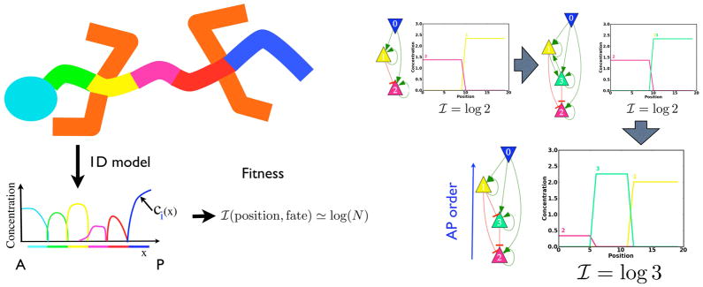
Computational evolution of AP patterning in metazoans [40]. A. The body plan is idealized as a succession of non-overlapping gene expression territories. The fitness is the mutual information, I, between gene identity (construed as a probability) and AP position [40]. For N patterning genes, the mutual information is maximal and equal to log(N) when the genes have equal sized expression domains. B. Gene duplication and parameter refinement increases the number of territories by one along a path with non-decreasing mutual information. The imposed morphogen that increases from anterior to posterior is the purple gene 0. The patterning genes are shown as red, green, yellow from anterior to posterior.
The simulations in [40] selected at the end, many different networks all of which displayed the properties of temporal co-linearity and posterior prevalence and furthermore rationalize why these properties occur together. The simulation recruited a timer gene, whose level maps the time a cell spends in the posterior growth zone to morphogen level and hence gene expression. A similar effect may occur for sonic hedgehog [42, 43]. This mechanism incidentally provides an evolutionary path to explain the repeated emergence of long germ insects from their short germ ancestors; the timer gene becomes the posterior morphogen [37, 44]. This can occur progressively; the morphogen becomes static, but increases posteriorly, as more of the abdomen is patterned contemporaneously with anterior segments. A timer gene also provides a single control point where patterning can be kept in synchrony with growth when the latter changes by 2x with temperature in amphibians.
Simulations that optimize the mutual information between position and gene expression starting from the timer plus wavefront pre-pattern or boundary condition, are a good illustration of the power of this method to quantitatively tie together distinct phenotypes and suggest paths for large-scale evolutionary transitions [45].
The Hox genes are patterned in registry with the somites [46], and reference [47] evolves both networks together. If we allow for long-distance mutual activation of domains (via diffusion), there is no need for external timer: a reaction-diffusion model for somitogenesis can be generalized to many fates and a cascade of auto-activating genes can give rise to a sequence of mutually excluding domain. [27]
Discussion
A complete phenotype must include dynamics and then its mathematical expression is often not obvious. Computational evolution has proven to be a potent heuristic tool to generate dynamic models of development that cannot be written down by informal means. The models make novel but testable predictions about macro-evolution yet are simple enough to furnish a minimal parameterization of the dynamical phenotype that can be fit to data in a non-redundant way. Experiment can affirm or falsify an evolved model, but failure to evolve a model says nothing about its validity. There is no proof that computational evolution explores all alternatives.
The nominal fitness that we optimize computationally, has nothing to do with reproductive success, and merely defines the pattern we wish to create in generic terms. Both computational and organic evolution are incremental and the functions we optimize all confer some benefit on the earliest pattern, admit iterative improvement by a local search, and eventually saturate. By analogy, a protein does not sample all possible configurations as it folds, but moves down a free energy funnel. Although we do not know the mutation rates for processes that affect phenotypic change, what matters is the network at the bottom of the funnel and a search process that samples the local environment densely enough to find a path down hill. When the desired phenotype is naturally expressed as several criteria, Pareto optimization (http://en.wikipedia.org/wiki/Pareto_efficiency) is as applicable to evolution as it is to sociology (A. Warmflash et. al. Phys. Bio. to appear)
It is noteworthy that with plausible parameters, the evolution of complex phenotypes can be very rapid when guided by continual fitness increases before saturating to a local optimum [48]. Computational evolution of phenotype generates precisely those networks that can be learned by an incremental search that mimics natural evolution, so the explosion of new phyla during the Cambrian is perhaps not such a mystery.
Acknowledgments
PF was supported by Natural Science and Engineering Research Council of Canada (NSERC), Discovery Grant program RGPIN 401950-11, Regroupement Québécois pour les matériaux de pointe (RQMP) and McGill University. EDS was supported by NSF grant PHY-0954398. Francis Corson supplied Fig. 2.
Glossary
- Geometry
representation of dynamics by a field of arrows (flow) often in an abstract space, where the axes correspond to signaling pathways controlling fates
- Attractor
When all external parameters of a given system are fixed, its state will asymptotically converge in time toward a stable attractor. Examples of attractors include stable fixed points or limit-cycles for oscillating systems
- Bistability
a system characterized by the existence of two stable fixed points. A third fixed point also exists but is unstable, i.e. any local perturbation will push the system to one of the two other fixed points
- Bifurcation
a qualitative change of the attractor of the dynamics (e.g. from oscillating to non oscillating) after a change of parameter. This is the dynamical system analog to a phase transition in physics (e.g. water to ice)
- Hopf Bifurcation
a bifurcation from a stable fixed point to an oscillating system
- Saddle-node bifurcation
a bifurcation resulting in the appearance of an extra stable fixed point for the dynamics. Typically an unstable fixed point must appear as well. If there is no symmetry in the system, transitions from monostable dynamics to bistable ones are saddle-node bifurcation
- Fitness
the generic term from the field of genetic programming [11] to designate the scoring function(s) that is optimized by the computation
Footnotes
Publisher's Disclaimer: This is a PDF file of an unedited manuscript that has been accepted for publication. As a service to our customers we are providing this early version of the manuscript. The manuscript will undergo copyediting, typesetting, and review of the resulting proof before it is published in its final citable form. Please note that during the production process errors may be discovered which could affect the content, and all legal disclaimers that apply to the journal pertain.
References
- 1.Slack JMW. Developmental and cell biology series. 2. xix. Cambridge [England]; New York: Cambridge University Press; 1991. From egg to embryo: regional specification in early development; p. 328. [Google Scholar]
- 2.Slack JMW. Conrad Hal Waddington: the last Renaissance biologist? Nat Rev Genet. 2002;3(11):889–895. doi: 10.1038/nrg933. [DOI] [PubMed] [Google Scholar]
- 3.Daniels BC, et al. Sloppiness, robustness, and evolvability in systems biology. Current Opinion in Biotechnology. 2008;19(4):389–395. doi: 10.1016/j.copbio.2008.06.008. [DOI] [PubMed] [Google Scholar]
- 4.Cherry JL, Adler FR. How to make a biological switch. Journal of Theoretical Biology. 2000;203(2):117–133. doi: 10.1006/jtbi.2000.1068. [DOI] [PubMed] [Google Scholar]
- 5.Gardner TS, Cantor CR, Collins JJ. Construction of a genetic toggle switch in Escherichia coli. Nature. 2000;403(6767):339–342. doi: 10.1038/35002131. [DOI] [PubMed] [Google Scholar]
- 6.Laslo P, et al. Multilineage Transcriptional Priming and Determination of Alternate Hematopoietic Cell Fates. Cell. 2006;126(4):755–766. doi: 10.1016/j.cell.2006.06.052. [DOI] [PubMed] [Google Scholar]
- 7.Losick R, Desplan C. Stochasticity and cell fate. Science. 2008;320(5872):65–8. doi: 10.1126/science.1147888. [DOI] [PMC free article] [PubMed] [Google Scholar]
- 8.Francois P, Hakim V. Design of genetic networks with specified functions by evolution in silico. Proc Natl Acad Sci U S A. 2004;101(2):580–5. doi: 10.1073/pnas.0304532101. [DOI] [PMC free article] [PubMed] [Google Scholar]
- 9.Soyer OS, Pfeiffer T, Bonhoeffer S. Simulating the evolution of signal transduction pathways. J Theor Biol. 2006;241(2):223–32. doi: 10.1016/j.jtbi.2005.11.024. [DOI] [PubMed] [Google Scholar]
- 10.Goldstein RA, Soyer OS. Evolution of taxis responses in virtual bacteria: non-adaptive dynamics. PLoS Comput Biol. 2008;4(5):e1000084. doi: 10.1371/journal.pcbi.1000084. [DOI] [PMC free article] [PubMed] [Google Scholar]
- 11.Holland JH. Adaptation in natural and artificial systems: an introductory analysis with applications to biology, control, and artificial intelligence. viii. Ann Arbor: University of Michigan Press; 1975. p. 183. [Google Scholar]
- 12.Katagiri T, et al. Bone morphogenetic protein-2 converts the differentiation pathway of C2C12 myoblasts into the osteoblast lineage. J Cell Biol. 1994;127(6 Pt 1):1755–66. doi: 10.1083/jcb.127.6.1755. [DOI] [PMC free article] [PubMed] [Google Scholar]
- 13.Orkin SH, Zon LI. Hematopoiesis: an evolving paradigm for stem cell biology. Cell. 2008;132(4):631–44. doi: 10.1016/j.cell.2008.01.025. [DOI] [PMC free article] [PubMed] [Google Scholar]
- 14.Graf T, Enver T. Forcing cells to change lineages. Nature. 2009;462(7273):587–594. doi: 10.1038/nature08533. [DOI] [PubMed] [Google Scholar]
- 15.Corson F, Siggia ED. Geometry, epistasis, and developmental patterning. Proc Natl Acad Sci U S A. 2012;109(15):5568–75. doi: 10.1073/pnas.1201505109. [DOI] [PMC free article] [PubMed] [Google Scholar]
- 16.Jaeger J, et al. Dynamical analysis of regulatory interactions in the gap gene system of Drosophila melanogaster. Genetics. 2004;167(4):1721–1737. doi: 10.1534/genetics.104.027334. [DOI] [PMC free article] [PubMed] [Google Scholar]
- 17.Rouault H, Hakim V. Different cell fates from cell-cell interactions: core architectures of two-cell bistable networks. Biophysical Journal. 2012;102(3):417–426. doi: 10.1016/j.bpj.2011.11.4022. [DOI] [PMC free article] [PubMed] [Google Scholar]
- 18* (Francois 2007).Francois P, Hakim V, Siggia ED. Deriving structure from evolution: metazoan segmentation. Mol Syst Biol. 2007;3:154. doi: 10.1038/msb4100192. A dynamical model for somitogenesis was derived by computational evolution, that can readily be reduced to a sequence of bifurcations. [DOI] [PMC free article] [PubMed] [Google Scholar]
- 19.Cooke J, Zeeman EC. A clock and wavefront model for control of the number of repeated structures during animal morphogenesis. Journal of Theoretical Biology. 1976;58(2):455–476. doi: 10.1016/s0022-5193(76)80131-2. [DOI] [PubMed] [Google Scholar]
- 20.Aulehla A, Pourquié O. Signaling Gradients during Paraxial Mesoderm Development. Cold Spring Harbor Perspectives in Biology. 2010;2(2):1–17. doi: 10.1101/cshperspect.a000869. [DOI] [PMC free article] [PubMed] [Google Scholar]
- 21.Oates AC, Morelli LG, Ares S. Patterning embryos with oscillations: structure, function and dynamics of the vertebrate segmentation clock. Development. 2012;139(4):625–39. doi: 10.1242/dev.063735. [DOI] [PubMed] [Google Scholar]
- 22** (Krol 2011).Krol AJ, et al. Evolutionary plasticity of segmentation clock networks. Development (Cambridge, England) 2011;138(13):2783–2792. doi: 10.1242/dev.063834. Genes whose expression oscillates during somitogenesis are compared among fish, chick and mouse with little overlap found, though the phenotype of patterning identical. Models built around individual genes are species specific while geometric models emphasize the broad features of phenotype. [DOI] [PMC free article] [PubMed] [Google Scholar]
- 23.Takahashi Y, et al. Mesp2 initiates somite segmentation through the Notch signalling pathway. Nat Genet. 2000;25(4):390–6. doi: 10.1038/78062. [DOI] [PubMed] [Google Scholar]
- 24.Morimoto M, et al. The Mesp2 transcription factor establishes segmental borders by suppressing Notch activity. Nat Cell Biol. 2005;435(7040):354–359. doi: 10.1038/nature03591. [DOI] [PubMed] [Google Scholar]
- 25* (Oginuma 2010).Oginuma M, et al. The oscillation of Notch activation, but not its boundary, is required for somite border formation and rostral-caudal patterning within a somite. Development (Cambridge, England) 2010;137(9):1515–1522. doi: 10.1242/dev.044545. An experimental study showing how phase information from the clock (via Notch signaling) is retained to define rostro-caudal polarity in the somites. [DOI] [PubMed] [Google Scholar]
- 26.Goldbeter A, Gonze D, Pourquié O. Sharp developmental thresholds defined through bistability by antagonistic gradients of retinoic acid and FGF signaling. Developmental dynamics: an official publication of the American Association of Anatomists. 2007;236(6):1495–1508. doi: 10.1002/dvdy.21193. [DOI] [PubMed] [Google Scholar]
- 27.Meinhardt H. Models of Biological pattern formation. Academic Press; 1982. [Google Scholar]
- 28.Hester SD, et al. A multi-cell, multi-scale model of vertebrate segmentation and somite formation. PLoS Comput Biol. 2011;7(10):e1002155. doi: 10.1371/journal.pcbi.1002155. [DOI] [PMC free article] [PubMed] [Google Scholar]
- 29.Hughes DST, Keynes RJ, Tannahill D. Extensive molecular differences between anterior- and posterior-half-sclerotomes underlie somite polarity and spinal nerve segmentation. BMC developmental biology. 2009;9:30. doi: 10.1186/1471-213X-9-30. [DOI] [PMC free article] [PubMed] [Google Scholar]
- 30.Henry CA, et al. Somites in zebrafish doubly mutant for knypek and trilobite form without internal mesenchymal cells or compaction. Current biology: CB. 2000;10(17):1063–1066. doi: 10.1016/s0960-9822(00)00677-1. [DOI] [PubMed] [Google Scholar]
- 31.Santillán M, Mackey MC. A proposed mechanism for the interaction of the segmentation clock and the determination front in somitogenesis. PLoS ONE. 2008;3(2):e1561. doi: 10.1371/journal.pone.0001561. [DOI] [PMC free article] [PubMed] [Google Scholar]
- 32.Ferrell JE, Jr, et al. Simple, realistic models of complex biological processes: positive feedback and bistability in a cell fate switch and a cell cycle oscillator. FEBS Lett. 2009;583(24):3999–4005. doi: 10.1016/j.febslet.2009.10.068. [DOI] [PubMed] [Google Scholar]
- 33.Cross FR. Two redundant oscillatory mechanisms in the yeast cell cycle. Dev Cell. 2003;4(5):741–52. doi: 10.1016/s1534-5807(03)00119-9. [DOI] [PubMed] [Google Scholar]
- 34.Palmeirim I, et al. Avian hairy gene expression identifies a molecular clock linked to vertebrate segmentation and somitogenesis. Cell. 1997;91(5):639–648. doi: 10.1016/s0092-8674(00)80451-1. [DOI] [PubMed] [Google Scholar]
- 35* (Aulehla,2008).Aulehla A, et al. A beta-catenin gradient links the clock and wavefront systems in mouse embryo segmentation. Nat Cell Biol. 2008;10(2):186–193. doi: 10.1038/ncb1679. A real time imaging strategy has been used in mouse to visualize the segmentation clock in real time and links it to the Wnt morphogen gradient. [DOI] [PMC free article] [PubMed] [Google Scholar]
- 36.Keller PJ, et al. Reconstruction of zebrafish early embryonic development by scanned light sheet microscopy. Science. 2008;322(5904):1065–9. doi: 10.1126/science.1162493. [DOI] [PubMed] [Google Scholar]
- 37** (Sarrazin 2012).Sarrazin AF, Peel AD, Averof M. A segmentation clock with two-segment periodicity in insects. Science. 2012;336(6079):338–341. doi: 10.1126/science.1218256. First demonstration of the existence of a segmentation clock coupled to growth in short germ insects. [DOI] [PubMed] [Google Scholar]
- 38.Kmita M, Duboule D. Organizing axes in time and space; 25 years of colinear tinkering. Science. 2003;301(5631):331–333. doi: 10.1126/science.1085753. [DOI] [PubMed] [Google Scholar]
- 39.McGinnis W, Krumlauf R. Homeobox genes and axial patterning. Cell. 1992;68(2):283–302. doi: 10.1016/0092-8674(92)90471-n. [DOI] [PubMed] [Google Scholar]
- 40* (Francois 2010).François P, Siggia ED. Predicting embryonic patterning using mutual entropy fitness and in silico evolution. Development (Cambridge, England) 2010;137(14):2385–2395. doi: 10.1242/dev.048033. A generic fitness that favors gene expression in specific spatial locations was optimized and yielded gene networks whose phenotypes resembled Hox genes. [DOI] [PubMed] [Google Scholar]
- 41.Wacker SA, et al. Timed interactions between the Hox expressing non-organiser mesoderm and the Spemann organiser generate positional information during vertebrate gastrulation. Developmental Biology. 2004;268(1):207–219. doi: 10.1016/j.ydbio.2003.12.022. [DOI] [PubMed] [Google Scholar]
- 42.Tabin C, Wolpert L. Rethinking the proximodistal axis of the vertebrate limb in the molecular era. Genes & Development. 2007;21(12):1433–1442. doi: 10.1101/gad.1547407. [DOI] [PubMed] [Google Scholar]
- 43* (Balaskas 2012).Balaskas N, et al. Gene Regulatory Logic for Reading the Sonic Hedgehog Signaling Gradient in the Vertebrate Neural Tube. Cell. 2012;148(1–2):273–284. doi: 10.1016/j.cell.2011.10.047. Vertebrate neural tube patterning is shown to be controlled by timing of Shh dynamics. A nice example of bistability and hysteresis in developmental networks. [DOI] [PMC free article] [PubMed] [Google Scholar]
- 44.Peel AD. The evolution of developmental gene networks: lessons from comparative studies on holometabolous insects. Philosophical transactions of the Royal Society of London Series B, Biological sciences. 2008;363(1496):1539–1547. doi: 10.1098/rstb.2007.2244. [DOI] [PMC free article] [PubMed] [Google Scholar]
- 45.Nahmad M, Glass L, Abouheif E. The dynamics of developmental system drift in the gene network underlying wing polyphenism in ants: a mathematical model. Evolution & Development. 2008;10(3):360–374. doi: 10.1111/j.1525-142X.2008.00244.x. [DOI] [PubMed] [Google Scholar]
- 46.Iimura T, Pourquié O. Hox genes in time and space during vertebrate body formation. Dev Growth Differ. 2007;49(4):265–275. doi: 10.1111/j.1440-169X.2007.00928.x. [DOI] [PubMed] [Google Scholar]
- 47.ten Tusscher KH, Hogeweg P. Evolution of Networks for Body Plan Patterning; Interplay of Modularity, Robustness and Evolvability. PLoS Comput Biol. 2011;7(10):e1002208. doi: 10.1371/journal.pcbi.1002208. [DOI] [PMC free article] [PubMed] [Google Scholar]
- 48.Nilsson DE, Pelger S. A pessimistic estimate of the time required for an eye to evolve. Proc Biol Sci. 1994;256(1345):53–58. doi: 10.1098/rspb.1994.0048. [DOI] [PubMed] [Google Scholar]