Pareto Evolution of Gene Networks: An Algorithm to Optimize Multiple Fitness Objectives

Abstract

The computational evolution of gene networks functions like a forward genetic screen to generate, without preconceptions, all networks that can be assembled from a defined list of parts to implement a given function. Frequently networks are subject to multiple design criteria that can’t all be optimized simultaneously. To explore how these tradeoffs interact with evolution, we implement Pareto optimization in the context of gene network evolution. In response to a temporal pulse of a signal, we evolve networks whose output turns on slowly after the pulse begins, and shuts down rapidly when the pulse terminates. The best performing networks under our conditions do not fall into the categories such as feed forward and negative feedback that also encode the input-output relation we used for selection. Pareto evolution can more efficiently search the space of networks than optimization based on a single ad-hoc combination of the design criteria.

Introduction

The concept of Pareto optimality arises naturally in the context of economics or game theory when one is faced with the problem of optimizing a system according to multiple criteria. With two criteria, we can plot the performance of all systems in the plane and two qualitative outcomes are possible (figure 1). Typically there are tradeoffs, and the Pareto frontier is the curve along which it is impossible to minimize one criterion without increasing the other. Exceptionally there will be a single point that optimizes both criteria. In a rational world all economies would operate on the Pareto frontier, and politics would decide the operating point along the frontier (http://en.wikipedia.org/wiki/Pareto_efficiency).

Figure 1.

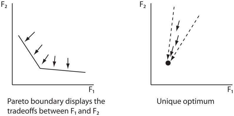
Map from the space all models into the Pareto fitness plane (assuming smaller is better). There are typically tradeoffs between the two functions being minimized, but exceptionally one or more models are optimal for both functions.

Tradeoffs are inherent in all biological processes from metabolism to environmental response see e.g. (El-Samad, Kurata et al. 2005). Pareto optimality, as one formalization of tradeoffs, has seen less application in evolution since it appears axiomatic that reproductive fitness alone is to be optimized. Of course there are multiple tradeoffs implicit in any organism, but they are hard to disaggregate and quantify. A more accessible source of bio-mimetic optimization problems with multiple criteria is the computational evolution of gene networks defined in functional, input-output terms. Adaptive networks, for instance, register temporal changes in input, but relax to a unique fixed point when the input is constant. Adaptive circuits thus need to optimize two criteria (1) a large output response to a step in input (2) a small difference between the output levels well before and after the step (Francois and Siggia 2008; Ma, Trusina et al. 2009).

There is often no intuitive or unique way to combine multiple fitness criteria and an ad-hoc fitness function is chosen without justification. Thus computing the Pareto frontier makes the tradeoffs among the fitness criteria explicit and for the problem we consider here reveals that certain topologies cluster along the frontier. A single ad-hoc fitness function can simply loose certain solutions by imposing an arbitrary selection along the frontier. Pareto computation can also speed up evolutionary simulations as the greater flexibility to move in Pareto space can help to overcome barriers. (Adaptation, is unusual in that it corresponds to the situation in figure 1B with a unique optimum on the Pareto frontier (Francois and Siggia 2008), i.e., there is a path in parameter space starting from any point that optimizes both fitness criteria.)

One of the major goals of systems biology is to assign functions to biological networks that are still incompletely described. We know more about their topology (i.e., what is connected to what) than the numbers describing these connections and we know more about transcription than mRNA regulation or post-translational protein modifications. While it is tempting to suggest that a network has evolved to perform particular functions, without considering the evolutionary history of such networks these rationalizations run the risk of being “just-so” stories (Lynch 2007). Computational evolution (Francois and Hakim 2004; Soyer, Pfeiffer et al. 2006; Goldstein and Soyer 2008) is an antidote to such reasoning and functions much like a forward genetic screen. One poses a phenotype and the computer returns networks that implement it. These networks can then be compared, using various measures, with those seen in biology.

Here we modify our previously described evolutionary algorithm (Francois, Hakim et al. 2007; Francois and Siggia 2008; Francois and Siggia 2010) to encompass Pareto evolution. In cases where the fitness functions cannot be simultaneously optimized, Pareto evolution allows one to identify a group of networks on the Pareto front some of which would have been passed over by particular combinations of the fitness functions

Algorithm

In previous papers (Francois, Hakim et al. 2007; Francois and Siggia 2008; Francois and Siggia 2010), we developed an algorithm to evolve gene networks. Transcriptional interactions are described by Michaelis-Menten-Hill kinetics and post-transcriptional interactions by mass-action laws (Supplement). In the simplest case, that suffices here, simulations are initialized with two variables, an input gene that presents a prescribed signal and an output gene whose behavior in response to the input defines the fitness. The simulation then builds a network connecting the input and output adjusting both the topology and kinetic parameters to optimize the fitness. In the present work, we restrict genes to interact only through transcriptional regulations or protein-protein interactions (PPI). All details of the network implementation are unchanged from (Francois and Siggia 2010) and recapitulated in the Supplement. Selection was previously imposed by computing the fitness for all networks in the population, discarding the least fit half of the population and replacing it with a mutated variant of the remaining half. (To preserve the analogy with energy, we assume the fitness is to be minimized.)

The selection step now has to be modified for Pareto optimization of multiple fitnesses, subsequently called Pareto evolution. We say network-A Pareto dominates network-B if and only if it has a lower or equal fitness score for all fitness functions with at least one function being lower. To perform the Pareto evolution, we use the Goldberg algorithm (Van Veldhuizen and Lamont 2000) (Coello Coello, Van Veldhuizen et al. 2002) which ranks networks into discrete groups. Networks are evaluated separately for each of the fitness criteria and then networks that are not Pareto dominated by any other network are identified and assigned a rank of 1. These networks are then removed from consideration and the process is repeated. Networks identified in the second round are assigned a Pareto rank of 2 and then removed from consideration. The process repeats until all networks have been assigned a Pareto rank.

Following this procedure, the Pareto rank scores of networks are modified using a fitness-sharing algorithm. The goal of this is to reduce the score of networks that lie too close together in the fitness space thus promoting greater diversity among the networks that are retained in each generation. This is achieved by raising the Pareto rank score (P_i) of a network i whenever other networks are located within a defined radius r_s in the fitness space according to:

$$\mathrm{\Delta }{P}_i=\frac{1}{N}\sum _{j\ne i}(1-d_{ij}/r_s)$$

where d_ij is the distance between networks i and j in the fitness space, N is the total number of networks, and r_s is a fixed parameter. This choice ensures that networks of Pareto rank 1 remain above Pareto rank 2 but prioritizes those networks that are farthest from the others in fitness space. The best-ranked half of the population is retained and a copy of each of these networks is mutated and returned to the population.

Results

There are many situations in which it is advantageous for a system to respond with different timescales to the onset and termination of a signal. One application is to noise filtering – if a system is slow to turn on but rapidly shuts off, transient signals will be unable to activate the system. The coherent feed forward loop (FFL) has been suggested to play this role in biological systems (Mangan and Alon 2003), as it does in engineered systems

We used Pareto computational evolution to evolve networks that respond slowly to the onset of a signal and but rapidly upon its termination. The two fitness functions were chosen simply to be the negative ON-time, −t_ON and the OFF-time, t_OFF and evolution then minimizes these functions. To define the response times, we adapted the most stringent definitions possible. Since we maximize the ON-time it is defined by when the value of the output changes by just 5% from its prior steady value. The OFF-time, to be minimized, is defined as the time necessary to attain 5% of the new steady state value.

We do not specify whether high input induces high output or the converse, only the response times are selected.

Since we are selecting on actual times, not ratios, the fitness depends unavoidably on all the parameters that involve time. The simulation imposes upper limits of order one on all network parameters with the dimensions of inverse time. Rate dependent quantities include obviously the protein degradation rate, the transcription rate, but also (together with concentration) the rate for PPI. If we included catalytic processes, there would be other intrinsic maximum rates. This is true biochemically as well as in simulations, and it is to be expected that extrinsic bounds on reaction rates will impact the gene networks that evolution selects to encode a response defined in input-output terms.

The optimal degradation process in the simulations below always evolves to be PPI of the output with itself. Both the maximum PPI association rate and the protein degradation rate are one in our units, but the protein concentration is not limited to one and making a homodimer from the output results in more rapid response at high output levels. Conventional protein degradation remains more efficient at low output levels and is present in all cases, but does not merit a link in our network topology graph. We did not anticipate that PPI would accelerate the response time, but it could well happen in vivo (Buchler and Louis 2008) and is an example of how simulations can stimulate one’s imagination.

During evolution, networks readily spread out in fitness space and define the Pareto front (figure 2A). To uncover the limits of a given topology on the Pareto fitness plane it is convenient to fix the topology with one of the evolved networks and run the evolution code, allowing only parameter changes (figure 2B). For the two evolved networks that achieve t_ON order ten, there are in fact no points in the abscissa range [−4, 0], which is due to our finite population size. The Pareto frontier is nearly flat in all three cases. Since most points are pushed to the left during evolution, the few points that remain for −t_ON in [−4, 0] are eliminated by any point with an infinitesimally smaller t_OFF and a larger t_ON.

Figure 2.

The Pareto frontier for the evolution of slow ON, fast OFF networks. (A) As a function of generation number, the networks spread down and to the left, showing improved fitness. (B) Parameters are Pareto optimized separately for fixed topology to display the fitness limits of each topology. The feed forward loop (FFL), cascade (Cscd), and positive feedback (PFB) networks appear in Figure 3. The two networks in the blow up around the origin, the Input+Output PPI (PPI) and negative autoregulation (NFB) are shown in figure 4

The three networks in figure 2B that achieve the largest t_ON are discussed immediately below, followed by those that occupy the corner around (0,0).

Many of networks below have been studied before, reviewed in (Kholodenko 2006; Alon 2007). Our emphasis here is to extend the scope of in-silico simulations, so we discuss network dynamics only as it pertains to the fitness criterion we are optimizing.

A. Cascade

The most effective network that implements the slow on fast off function is a simple two step cascade with an intermediate buffer mode, schematically: I--| B--|O where I is the input, B is the buffer, and O is the output. The second arrow can be either activation or repression depending on whether the input and output are correlated or anti-correlated. The system is most effective when B is expressed at high levels and the threshold for the response of O to B is very low.

Thus when the input turns on (figure 3A, S_A is the buffer), there is a long lag before B drops low enough for O to respond. On the contrary, when the input turns off, B quickly reaches a level high enough for O to turn on again. Reactivation of O is faster if the intrinsic time scale of O is short and its production rate is high. (It also helps that the repression of O by B is cooperative i.e., has a high Hill exponent.)

Figure 3.

Details of the three networks with the largest ON time in figure 2 in order of decreasing fitness. Single lines terminating with an arrow or bar denote transcription activation/repression. Merging lines denote PPI. Thus O₂ is a dimer of the output. (A) The cascade (Cscd) functions with a buffer, S_A, that builds up to a large value. Its decay defines the ON time for the output. (B) In the positive feedback (PFB) S_B accumulates slowly until it reaches the threshold necessary to activate S_A. (C) A feed forward loop (FFL) with the AND operation between S_A and the input made explicit with a PPI. The decay in all cases is by PPI for the reasons explained in the text.

The evolutionary path leading to the cascade network in figure 3A is instructive since in outline, it is followed by the other networks that achieve a large t_ON. The fast t_OFF, mediated by the PPI, evolves first and generates networks along the diagonal emanating from the origin in figure 2A. There is still a direct transcriptional connection from the input to the output. Neutral evolution, via several routes, generates an activator connected to the output. The input then represses this activator and the direct connection between input and output (along with miscellaneous other transcriptional and PPI connections) are later lost. Any expansion of Pareto frontier to t_ON > 50 (along with a departure from the linear relation between t_OFF and t_ON) is associated with the appearance of one or more species between the input and output.

Cascade networks are seldom as simple as our schematic I--| B--|O, since they may be decorated with other interactions that are marginally functional and have not yet disappeared, or whose benefit is contingent on earlier steps in evolution. Individual topologies can be ‘pruned’ i.e., evolved in a regime where interactions are removed but never added, to uncover their core. But cascades are most easily identified by following the time course and identifying the buffer variable.

B. Positive feedback

An example of a network utilizing positive feedback to turn on with a delay is shown in figure 3B. Upon activation, the input complexes with another component S_A and this complex, S_B, activates the output. Importantly S_B is also required to produce S_A generating a positive feedback loop. The effect of this positive feedback loop is to create non-linear activation, that slows the response when I increases. In addition S_B is subject to a strong threshold (i.e., high Hill exponent) when it turns on O. Thus any effect on O is delayed until S_B gets over some threshold. When the input drops to zero as in figure 3B, production of S_B abruptly ceases and a large decay rate reduces S_B to zero. Additionally, in some simulations, the input evolves to directly repress S_A adding an additional barrier to be overcome by the positive feedback and further delaying the activation of the output.

C. Feed forward dynamics

This did not evolve directly in our simulations, but we initialized the topology and optimized parameters (figure 3C). It is then apparent from figure 2B that under Pareto optimization its performance is inferior to other topologies. This, as always, can be an artifact of our defined parameter ranges (the same for all networks) or the components from which we build networks. (Conditions favoring a FFL were found in (Dekel, Mangan et al. 2005).) In particular we use a PPI to impose an AND operation between the input and a secondary transcriptional target of the input, and then use the resulting complex to control the output. Thus the t_OFF does not track the input as it would if the AND operation was instantaneous, and t_OFF is not necessarily shorter than for a cascade. As before, a PPI of the output with itself gives optimal response times at the termination of the signal.

The following networks are marginally inferior to the cascade network for small t_ON but appear in the simulations since they are quick to evolve in figure 2A and cluster around the origin. They have the feature that t_ON and t_OFF are coupled.

D. Negative autoregulation

Figure 4A shows a network in which the input directly influences the output that negatively autoregulates. It was frequently selected because of the rapid jump in output level following the shutoff of signal (Rosenfeld, Elowitz et al. 2002). These networks have fast OFF but moderate ON times and thus fall on one corner of Pareto frontier (figure 2B).

Figure 4.

Two networks modest ON times and a single time scale from figure 2. (A) Negative auto regulation is slightly less fit than the double PPI in (B), and would be worse for our parameter ranges if the degradation by PPI was replaced by linear exponential decay. (B) The balance between the strength of the repression and the two PPI determine the time scale. The dashed transcriptional repression has no effect on the Pareto frontier.

E. I+O PPI

Here the input and output interact via a PPI. This performs slightly better than negative autoregulation and identically to a variant with an additional repression, figure 4B.

Pareto evolution can speed convergence

We compared the results of Pareto evolution with those that used conventional evolution to minimize the ratio −t_ON/t_OFF (Figure 5). As noted above, in Pareto simulations, solutions to achieve low t_OFF evolve very rapidly (Figure 5, left panel) and conventional evolution never achieves similar low values. Networks with long t_ON also evolve more readily in Pareto evolution and fewer simulations spend many generations at a bottleneck with low values of t_ON (Figure 5, center panel). In either case, evolving networks with (−t_ON/t_OFF ) < −1 is a relatively low probability event and occurred in 6/30 simulations for Pareto and in 5/30 simulations for conventional evolution (Figure 5, right panel). Thus, Pareto evolution allows the simulation to rapidly spread across the frontier discovering networks with long t_ON or short t_OFF in almost every simulation and may be a general mechanism for speeding up evolutionary simulations as compared to using ad hoc combinations of fitness criteria.

Figure 5.

Comparison of Pareto and standard computational evolution. Each line represents a single simulation, blue corresponds to standard evolution while red corresponds to pareto. Shown are the best OFF time (left), ON time (center), and ratio (right) as a function of the number of generations.

Discussion

We have implemented a standard Pareto optimization algorithm to create networks with a long ON time and a short OFF time in response to a square input pulse. The networks were built from a combination of transcriptional and protein-protein interactions, and parameters were limited to defined ranges (Supplement)

It is very evident in the Pareto frontier plots in figure 2B that some networks effectively decouple the ON and OFF times. These all operate by a common mechanism. By various means, either through multiple reaction steps or accumulation/decay of a large buffer, t_ON becomes long. The t_OFF is short due to standard decay/sequestration processes acting directly on the output (i.e., not a network feature).

Simulations built around standard chemical kinetics for well mixed systems can not do justice the complexity of the cell biology of signaling. The rates at which the simulation samples new topologies, e.g., the rates to add or remove transcriptional or protein-protein interactions are chosen purely for numerical efficiency and not from actual phylogenies. Our choice of network building blocks, for instance, determined how we implemented feed forward dynamics. Our parameter ranges had the unanticipated consequence of favoring the removal of output protein by PPI at high output concentrations rather than relying solely on the usual linear decay.

These technical assumptions do not contradict biological reality. The notion that intrinsic biochemical rates determine gene network topologies is not new; it’s a standard explanation for the prevalence of protein phosphorylation in signal transduction. The involvement of PPI in accelerating the output response is a good example of the suggestive mechanisms that arise from forward computational searches, and it might even occur in a cell (Buchler and Louis 2008).

Computational network evolution is an important theoretical tool in biological modeling. The simulations serve as a check on any theory that would impute a function to naturally occurring gene networks. Although our outcomes are influenced by parameter choices, these biases are very different from the ascertainment biases implicit in the current literature. In analogy with forward genetics, simulations may reveal unanticipated shortcomings in the screen or fitness functions themselves. Our cascade motif achieved a long t_ON by building up a high buffer concentration and only affecting the output below a very low threshold. Thus if we wanted to impose a third Pareto constraint on the maximum protein level or its minimum (due to molecular noise?) the networks would be reordered along this direction.

We can validly conclude from the simulations that many topologies can give rise to similar performance and it seems very difficult to guess the function on which selection was acting from the topology. For instance (Rosenfeld, Elowitz et al. 2002) show that adding negative transcriptional feedback to gene activation can accelerate the response time by a factor of 5X for a fixed steady state protein level. They propose this mechanism to enhance the response since they assume the protein is stable and removed only by dilution. Of course in other contexts proteins are actively degraded, which is another route to a faster response. Similarly a FFL can lead to a slow ON fast OFF phenotype (Mangan, Zaslaver et al. 2003), but other topologies do perform better under the parameter constraints of our simulations. Reasons other than response times could explain the transcriptional control strategies that employ a FFL. In some cases the relevant transcription factors are controlled by small metabolites that add another level of regulation to production of the product.

Network evolution should be contrasted with exhaustive parameter search as a means of connecting networks to function e.g., see (von Dassow, Meir et al. 2000; Ma, Trusina et al. 2009; Cotterell and Sharpe 2010). Parameter search requires starting from a fixed topology, since parameters have to be defined before they can be searched. Exhaustive search places severe limits on the number of genes and interactions allowed since the former require at least two parameters (constitutive production and decay) and the latter three (Michaelis-Menten rate, concentration, Hill exponent). With four values for each parameter and four genes and interactions there are 10¹² parameter sets and minimally 10³ operations required to solve the differential equations for each set. If the assumption of a topology and the sparse parameter sampling that is done in practice were not problems enough, evolution does not uniformly sample parameter space, jumping directly from no function to optimal and back again. An analogy can be made to protein folding, which can not sample all possible bond angle configurations (Levinthal ‘paradox’) and then select to the best one (Dill, Ozkan et al. 2008). Both evolution and protein folding proceed via incremental improvement and sampling what is accessible by local search. Our simulations mimic this process and allow us to sample topologies and reach far larger systems than could be imagined with exhaustive parameter search, even if one could guess what topologies to search.

It is a truism that selection acts on phenotype. Thus if we abstract from the simulations not the network per se, but the dynamical properties of the network expressed geometrically such as bistability or adaptation then these constitute the phenotype. If the landscape is a funnel, then model parameters can influence how long it takes to reach the bottom, but not the ultimate destination. In more complex systems than we have evolved here, there was a unique succession of dynamical phenotypes, again with multiple networks capable of implementing each behavior (Francois, Hakim et al. 2007). This is a reflection of the adage that evolution rearranges what is currently available (‘bricolage’). At this level of generality the simulations might actually mimic nature.

References

- Alon U. An introduction to systems biology : design principles of biological circuits. Boca Raton, FL: Chapman & Hall/CRC; 2007. [Google Scholar]
- Buchler NE, Louis M. Molecular titration and ultrasensitivity in regulatory networks. J Mol Biol. 2008;384(5):1106–19. doi: 10.1016/j.jmb.2008.09.079. [DOI] [PubMed] [Google Scholar]
- Coello Coello CA, Van Veldhuizen DA, et al. Evolutionary algorithms for solving multi-objective problems. New York: Kluwer Academic; 2002. [Google Scholar]
- Cotterell J, Sharpe J. An atlas of gene regulatory networks reveals multiple three-gene mechanisms for interpreting morphogen gradients. Mol Syst Biol. 2010;6:425. doi: 10.1038/msb.2010.74. [DOI] [PMC free article] [PubMed] [Google Scholar]
- Dekel E, Mangan S, et al. Environmental selection of the feed-forward loop circuit in gene-regulation networks. Phys Biol. 2005;2(2):81–8. doi: 10.1088/1478-3975/2/2/001. [DOI] [PubMed] [Google Scholar]
- Dill KA, Ozkan SB, et al. The protein folding problem. Annu Rev Biophys. 2008;37:289–316. doi: 10.1146/annurev.biophys.37.092707.153558. [DOI] [PMC free article] [PubMed] [Google Scholar]
- El-Samad H, Kurata H, et al. Surviving heat shock: control strategies for robustness and performance. Proc Natl Acad Sci U S A. 2005;102(8):2736–41. doi: 10.1073/pnas.0403510102. [DOI] [PMC free article] [PubMed] [Google Scholar]
- Francois P, Hakim V. Design of genetic networks with specified functions by evolution in silico. Proc Natl Acad Sci U S A. 2004;101(2):580–5. doi: 10.1073/pnas.0304532101. [DOI] [PMC free article] [PubMed] [Google Scholar]
- Francois P, Hakim V, et al. Deriving structure from evolution: metazoan segmentation. Mol Syst Biol. 2007;3:154. doi: 10.1038/msb4100192. [DOI] [PMC free article] [PubMed] [Google Scholar]
- Francois P, Siggia ED. A case study of evolutionary computation of biochemical adaptation. Phys Biol. 2008;5(2):026009. doi: 10.1088/1478-3975/5/2/026009. [DOI] [PubMed] [Google Scholar]
- Francois P, Siggia ED. Predicting embryonic patterning using mutual entropy fitness and in silico evolution. Development. 2010;137(14):2385–95. doi: 10.1242/dev.048033. [DOI] [PubMed] [Google Scholar]
- Goldstein RA, Soyer OS. Evolution of taxis responses in virtual bacteria: non-adaptive dynamics. PLoS Comput Biol. 2008;4(5):e1000084. doi: 10.1371/journal.pcbi.1000084. [DOI] [PMC free article] [PubMed] [Google Scholar]
- Kholodenko BN. Cell-signalling dynamics in time and space. Nat Rev Mol Cell Biol. 2006;7(3):165–76. doi: 10.1038/nrm1838. [DOI] [PMC free article] [PubMed] [Google Scholar]
- Lynch M. The evolution of genetic networks by non-adaptive processes. Nat Rev Genet. 2007;8(10):803–13. doi: 10.1038/nrg2192. [DOI] [PubMed] [Google Scholar]
- Ma W, Trusina A, et al. Defining network topologies that can achieve biochemical adaptation. Cell. 2009;138(4):760–73. doi: 10.1016/j.cell.2009.06.013. [DOI] [PMC free article] [PubMed] [Google Scholar]
- Mangan S, Alon U. Structure and function of the feed-forward loop network motif. Proc Natl Acad Sci U S A. 2003;100(21):11980–5. doi: 10.1073/pnas.2133841100. [DOI] [PMC free article] [PubMed] [Google Scholar]
- Mangan S, Zaslaver A, et al. The coherent feedforward loop serves as a sign-sensitive delay element in transcription networks. J Mol Biol. 2003;334(2):197–204. doi: 10.1016/j.jmb.2003.09.049. [DOI] [PubMed] [Google Scholar]
- Rosenfeld N, Elowitz MB, et al. Negative autoregulation speeds the response times of transcription networks. J Mol Biol. 2002;323(5):785–93. doi: 10.1016/s0022-2836(02)00994-4. [DOI] [PubMed] [Google Scholar]
- Soyer OS, Pfeiffer T, et al. Simulating the evolution of signal transduction pathways. J Theor Biol. 2006;241(2):223–32. doi: 10.1016/j.jtbi.2005.11.024. [DOI] [PubMed] [Google Scholar]
- Van Veldhuizen DA, Lamont GB. Multiobjective Evolutionary Algorithms: Analysing the State-of-the-Art. Evolutionary Computation. 2000;8(2):125–147. doi: 10.1162/106365600568158. [DOI] [PubMed] [Google Scholar]
- von Dassow G, Meir E, et al. The segment polarity network is a robust developmental module. Nature. 2000;406(6792):188–92. doi: 10.1038/35018085. [DOI] [PubMed] [Google Scholar]
Associated Data
This section collects any data citations, data availability statements, or supplementary materials included in this article.