Noninvasive Intracranial Hypertension Detection Utilizing Semi-Supervised Learning

Abstract

Intracranial pressure (ICP) monitoring is an established clinical practice in managing patients with risk of acute ICP elevation although the clinically accepted way of measuring ICP remains invasive. However, the invasive nature of ICP measurement obviates its application in many clinical circumstances such as diagnosis of idiopathic intracranial hypertension (IIH). We propose a noninvasive diagnostic tool for intracranial hypertension (IH) based on the morphological analysis of cerebral blood flow velocity (CBFV) waveforms. We mainly compare two types of IH detection methods: one based on the traditional supervised learning approach and the other based on the semi-supervised learning approach. Our simulation results demonstrate that the predictive accuracy (area-under-the-curve) of the semi-supervised IH detection method can be as high as 92% while that of the supervised IH detection method is only around 82%. It should be noted that the predictive accuracy of the pulsatility index (PI) based IH detection method is as low as 59%. Although the predictive accuracy is a widely used accuracy measurement, it does not consider clinical consequences of necessary and unnecessary treatments. For this reason, we have adopted the decision curve analysis to address this issue. The decision curve analysis results show that the semi-supervised IH detection method is not only more accurate, but also clinically more useful than the supervised IH detection method or the PI-based IH detection method.

I. Introduction

Intracranial pressure (ICP) is a critical parameter for managing brain injury patients because timely detection of acute ICP elevation is needed to guide treatment to prevent severe complications including cerebral ischemia and herniation. Therefore, ICP monitoring is an established clinical practice in managing patients with risk of acute ICP elevation although the clinically accepted way of measuring ICP remains invasive. However, the invasive nature of ICP measurement obviates its application in many clinical circumstances where knowledge of ICP is of significant diagnostic and prognostic value but elevated ICP is either not life-threatening or an invasive procedure significantly increases the risk for patients. One example is the management of acute liver failure patients. Since coagulopathy (bleeding disorder) is common among patients with acute liver failure, the risks associated with invasive ICP monitoring outweigh the benefits of outcome prediction based on the invasive measurement of elevated ICP [1]. Another example is the diagnosis of idiopathic intracranial hypertension (IIH), which is rarely done by directly measuring ICP [2]. Therefore, the active search for a reliable noninvasive ICP monitoring technique has been conducted [3]–[7]. Despite such endeavors, none of them has demonstrated the significant clinical applicability. Several groups have also proposed a few simple metrics of CBFV such as maximum velocity, diastolic velocity, mean flow velocity, pulsatility index (PI), and resistance index for noninvasive assessment of ICP [8], [9]. It is, however, still controversial whether those simple metrics can provide reliable and accurate information about ICP [10], [11].

In acknowledgement of the limitations of the current noninvasive ICP assessment techniques we propose a noninvasive diagnostic tool for intracranial hypertension (IH) detection that utilizes the transcranial Doppler measurement of cerebral blood flow velocity (CBFV) at the middle cerebral arteries (MCAs). Recently, our group has conducted a quantitative study of the CBFV and ICP pulse morphology by integrating a whole array of novel morphological metrics [11]. Several morphological metrics from both pulses were found to be highly correlated in an inter-subject manner. This finding demonstrates a potential to develop alternative noninvasive ICP assessment methods based on a comprehensive morphological analysis of CBFV waveforms.

IH detection is a classification problem to differentiate patients with elevated ICP from those with normal (or low) ICP. The traditional approach to such classification problem is to use only labeled samples to train a given classifier, which is referred to as supervised learning. The major drawback of this approach is that it cannot utilize unlabeled samples even when useful information learned from them may result in the improvement of classification accuracy. Unlabeled samples may exist for various reasons such as the high cost or labor intensity of labeling all samples or the ambiguity in providing a binary label as in the case of IH detection. For an example, a naive approach would be to label CBFV waveforms as IH samples if the corresponding ICP is above 20 mmHg, which is a widely accepted threshold for considering ICP as elevated, and then to use a supervised learning algorithm to build the classifier. This straightforward paradigm may be too rigid making the detection of a true IH state critically dependent on the relevance of using 20 mmHg as a threshold. However, it is not an easy task to pick a different threshold, either. If the threshold is too high or too low, then one runs the risk of either missing IH diagnosis or creating too many false positives.

In order to address this ambiguity in labeling samples, we have adopted a new classification approach, that is, semi-supervised learning. In the semi-supervised learning it is not necessary to label all samples since classifiers can be trained using both labeled and unlabeled samples. There are several types of semi-supervised learning techniques including generative models, self-training, co-training, transductive support vector machines (SVM), and graph-based methods [12], [13]. Among them the graph-based semi-supervised learning techniques have drawn large attention due to their good performance and successful applications in visual and speech recognition [14], [15]. Specially, Spectral Regression technique proposed by Cai et al. has overcome several drawbacks of the conventional graph-based semi-supervised learning techniques by combining the ordinary regression technique with spectral graph analysis [16]. We have adopted their method to design our IH detection algorithm.

The objectives of the current study are to introduce a noninvasive IH detection method based on the TCD measurement of CBFV alone and to demonstrate its performance both in the supervised and semi-supervised learning settings.

II. Materials and Methodology

A. Data Collection

We collected ICP, CBFV, and ECG from 90 patients (ages: 18–92 [median: 47], gender: 47 male/43 female) admitted to neural-ICU and floor units at UCLA Medical Center between July 15, 2008 and November 16, 2011. Among them, 44 patients suffered from traumatic brain injury (TBI), 36 had aneurysmal subarachnoid hemorrhage (aSAH), and the rest were diagnosed with suspected normal pressure hydrocephalus (NPH). Table I summarizes patient’s diagnostic and demographic information.

TABLE I.

Summary of Patient Information.

		Gender
Diagnosis	Age	Female	Male
TBI	45 ± 15	18	26
aSAH	62 ± 12	21	15
NPH	59 ± 10	4	6

• TBI: traumatic brain injury
• aSAH: aneurysmal subarachnoid hemorrhage
• NPH: normal pressure hydrocephalus

ICP was measured invasively via continuous intracranial pressure monitoring for the clinical purpose using either intraventricular catheters for brain injury or intraparenchymal microsensors for NPH patients. Simultaneous cardiovascular monitoring was also performed using the bedside GE monitors. CBFV signals were obtained at the middle cerebral arteries (MCAs), which was ipsilateral to the ICP measurement location, while technicians affiliated with the Cerebral Blood Flow (CBF) laboratory at UCLA Department of Neurosurgery conducted daily clinical assessment of patients’ cerebral hemodynamics using transcranial Doppler (TCD). The duration of collected signals varies depending on how long the TCD monitoring of the MCAs could be done. Typically, the TCD monitoring lasted only 3–5 minutes since the probe had to be hand-held. This study was approved by Institutional Review Board (IRB) without involvement of any personal health information.

All signals were archived via a mobile cart equipped with the PowerLab data acquisition system (ADInstruments, Colorado Springs, CO), which samples analog signals from the bedside monitor at 400 Hz. Then, the archived signals were stored into the Chart™ binary file format for further analysis.

B. Morphological Clustering Analysis of Intracranial Pressure Pulses (MOCAIP)

We utilized the Morphological Clustering and Analysis of Intracranial Pressure Pulses (MOCAIP) algorithm to extract morphological features from TCD-based CBFV waveforms. The original intention of usage of MOCAIP was to extract a whole array of novel morphological features from ICP pulses [17]. Fig. 1 shows the block diagram of the MOCAIP algorithm. First, MOCAIP detects individual ICP pulses from a continuous ICP segment in association with a simultaneously recorded ECG segment [18]. After clustering the detected ICP pulses, MOCAIP recognizes valid (noise-free) pulses utilizing the ICP dominant pulse library, which contains 1435 dominant pulses [17]. Based on those recognized valid pulses, MOCAIP constructs one dominant pulse, which represents the majority of the pulses of the segment. Three sub-peaks, then, are optimally designated among several peak candidates. Fig. 2 illustrates a typical dominant pulse with six landmarks, {P₁, P₂, P₃, V₁, V₂, V₃}, which include three sub-peaks and three sub-troughs. A total of 128 metrics can be extracted in association with these landmarks such as latency, amplitude, curvature, slope, and ratios between them.

Fig. 1.

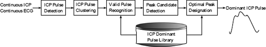
Block diagram of the Morphological Clustering and Analysis of Intracranial Pressure (MOCAIP) algorithm. Two inputs are continuous ICP and ECG segments and the output a dominant (representative) ICP pulse with three sub-peaks (this figure was adopted from [19] with the author’s permission).

Fig. 2.

An example of a dominant pulse, which is an output of MOCAIP, with six landmarks and basic features.

Previously, we have demonstrated that typical TCD-based CBFV waveforms are morphologically very similar (e.g. triphasic) to ICP pulses and thus MOCAIP can extract all 128 MOCAIP metrics from TCD-based CBFV waveforms successfully [11]. Plots in Fig. 3 illustrate typical CBFV dominant waveforms associated with various mean ICP values (5–33 mmHg): Top row (normal) and bottom row (hypertensive). Black dots represent three sub-peaks, which are optimally designated by MOCAIP.

Fig. 3.

Examples of CBFV dominant waveforms associated with various mean ICP values: Top row (normal) and bottom row (hypertensive). Black dots represent three sub-peaks, which are optimally designated by MOCAIP. CBFV dominant waveforms associated with low mean ICP values tend to have more distinct sub-peaks than those associated with high mean ICP pulses do. The difference between the second and third sub-peak amplitudes is greater in CBFV dominant waveforms associated with high mean ICP pulses than it is in those associated with normal mean ICP pulses.

C. Classification Technique: Spectral Regression Kernel Discriminant Analysis

The MOCAIP algorithm extracts various morphological features from TCD-based CBFV waveforms. Then, the next step is to learn the association rule (or function) between those CBFV MOCAIP features and corresponding labels (e.g. +1 for hypertensive samples and −1 for normal samples). It can be simply expressed as,

$$f(X_{n\times 128})\to Y_{n\times 1}$$ (1)

where X is a n×128 matrix of MOCAIP features, Y a n×1 vector of corresponding labels, n the number of samples, and f the association function or classifier to be learned or trained. The quality of the trained classifier is typically measured by its predictive accuracy. In other words, a good classifier is the one that can assign new features, which are unseen during training, into proper classes.

Cai et al. introduced a graph-based semi-supervised learning classification technique, called Spectral Regression [16]. It combines the ordinary regression technique with spectral graph analysis that was originally introduced as a clustering and dimensionality reduction technique [20]. In contrast to many conventional graph-based algorithms, which are transductive in nature, the Spectral Regression technique gives a natural out-of-sample extension both in the linear and kernel cases.

The first step of Spectral Regression is to compute a set of responses, y_i, for individual samples, x_i, by applying spectral techniques to a graph matrix. Once those responses are obtained, the ordinary ridge regression technique finds the regression function. The algorithmic procedure of Spectral Regression can be summarized as below,

1. Adjacency graph construction: Let G denote a graph with n nodes, where the i^th node represents the i^th sample, x_i. Construct the graph G by following three steps below,

   • Connect nodes i and j if they are among k nearest neighbors of each other.
   • Connect nodes i and j if they belong to the same class.
   • Remove the connection between i and j if they belong to different classes.
2. Weight matrix construction: Let W denote a sparse n×n matrix whose element W_i,j can be assigned as below,

   $$W_{i,j}=\{\begin{array}{cc}0\hfill & \text{if nodes }i\text{ and }j\text{ are not connected}\hfill \\ {1/l}^q\hfill & \text{if }{x}_i\text{ and }{x}_j\text{ belong to the same class}\hfill \\ s(i,j),\hfill & \text{otherwise}\hfill \end{array}$$

   where l^q is the number of samples that belong to the q^th class and s(i, j) a similarity function between x_i and x_j. Our choice of this similarity function was the heat kernel, that is,

   $$s(i,j)={\mathrm{e}}^{-\frac{{\Vert x_i-x_j\Vert }^2}{2{\sigma }^2}}$$ (2)
3. Eigen-decomposition: Find the largest eigenvectors of an eigen problem below,

   $$\mathit{\text{Wy}}=\lambda \mathit{\text{Dy}}$$ (3)

   where D is a diagonal matrix whose element D_i,i equals the sum of the i^th column of W.
4. Regularized least squares: Solve a regularized least squares problem for the p^th largest eigen vector y^p as below,

   $$a^p=\underset{a}{\text{argmin}}[{\displaystyle \sum _{i=1}^l}{(x_i^{\mathrm{T}}a-y_i^p)}^2+{\displaystyle \sum _{i=l+1}^n}{(\gamma x_i^{\mathrm{T}}a-y_i^p)}^2+\alpha {\Vert a\Vert }^2]$$ (4)

   where a is a regression coefficient vector, l the number of labeled samples, γ a parameter to adjust the weights of unlabeled samples, and α a regularization parameter. It is important to note that x_i is a sample vector while y_i a scalar response. By setting γ = 1, the closed form solution of a^p can be expressed as,

   $$a^p={({\mathit{\text{XX}}}^{\mathrm{T}}+\alpha I)}^{-1}{\mathit{\text{Xy}}}^p$$ (5)

One of many merits of Spectral Regression is that it provides a uniform learning approach. When samples are all labeled, Spectral Regression is essentially identical to Regularized Discriminant Analysis. In this case, the sparse matrix, W, becomes block-diagonal and the response, y, in Eq. (3) is equal to,

$$y^p={[\underset{{\displaystyle {\sum }_{i=1}^{p-1}}{l}^i}{\underbrace{0,\cdots ,0,}}\underset{l^p}{\underbrace{1,\cdots ,1,}}\underset{{\displaystyle {\sum }_{i=p+1}^c}{l}^i}{\underbrace{0,\cdots ,0}}]}^{\mathrm{T}}$$ (6)

where l^p is the number of samples that belong to the p^th class and c the total number of classes. On the other hand, when sample are all unlabeled, Spectral Regression becomes a spectral clustering technique with a natural out-of-sample extension capability, whose objective function is,

$$\text{min }{\displaystyle \sum _{i,j}}{\Vert y_i-y_j\Vert }^2{W}_{i,j}.$$ (7)

Eq. (7) indicates that the responses, y_i and y_j, should be close to each other when the i^th and j^th samples are similar. Belkin et al. have shown that the eigenvectors of the problem in Eq. (3) yield the optimal solution of the problem in Eq. (7) [21]. In the case of semi-supervised learning, Cai et al. have proved that the responses, y_i and y_j, as the solution of the eigen problem in Eq. (3) can be as close as possible when the i^th and j^th samples belong to the same class [16]. Such property is essential for semi-supervised learning since the same labeled samples are expected to have the same or similar responses.

Another important merit of Spectral Regression is that it can be easily extended into a nonlinear discriminant analysis by projecting all samples into the reproducing kernel Hilbert space (RKHS). Then, we can perform Spectral Regression in the high dimensional feature space and it is referred to as Spectral Regression Kernel Discriminant Analysis (SRKDA) [22]. In this case, the closed form solution of a^p in Eq. (5) becomes,

$$a^p={(K+\alpha I)}^{-1}{y}^p$$ (8)

where K is a n×n matrix, whose element K_i,j is 𝕂(x_i, x_j), and 𝕂(·, ·) the kernel function. Our choice of kernel was the Gaussian kernel. All experiments in our study were carried out utilizing SRKDA unless described otherwise. More details of the Spectral Regression algorithm can be found in [16], [22], [23].

There are two important parameters to be optimized in the SRKDA algorithm: Standard deviation of the heat kernel, σ, in Eq. (2) and that of the nonlinear (i.e. Gaussian) kernel function, 𝕂(·, ·). The standard deviation, σ, of the heat kernel was estimated as follows,

$$\mathrm{\sigma ̂}=\sqrt{\frac{1}{n-1}{\displaystyle \sum _{i=1}^n}{(x_i-\frac{1}{n}{\displaystyle \sum _{j=1}^n}{x}_j)}^2}$$ (9)

where n is the total number of training samples. The parameter, σ, could be optimized by running a separate cross-validation within a given training data set. However, there is a risk of over-tuning σ to a given training data set and compromising the generalizability of the model. In contrast, the estimate of σ in Eq. (9) is easy to obtain and its value happens to be quite similar to what could have been obtained by taking the cross-validation approach. For the same reason, the standard deviation of the Gaussian kernel function, 𝕂(·, ·), was estimated as in Eq. (9).

III. Experiment Design

A. Sample Labeling

ICP range was divided into three groups: normal (< 15 mmHg), grey-zone (15 mmHg–30 mmHg), and IH (> 30 mmHg). ICP remaining below 15 mmHg is assumed to be indicative of a normal state. In contrast, a patient’s condition is assumed to be at a greater risk when the ICP is beyond 30 mmHg.

As mentioned in section II-A, 3–5 minute long ICP and CBFV segments, which were simultaneously recorded during each session of daily cerebral hemodynamics assessment, were broken down into 1 minute segments. Each of these 1 minute segments contributes one sample, that is, a set of the 128 CBFV MOCAIP features. From 90 patients 131 sessions were collected and we could obtain a total of 563 samples. Those samples were assigned labels by applying the labeling criteria described above on the session level, not the sample level. In other words, if any of samples belonging to a given session meets the IH criterion, all samples of the session are labeled as IH. The rationale behind this labeling scheme is that what caregivers are most concerned about is whether a patient experiences IH at all during a given session. It is not so much of interest which of 1 minute segments during the session is associated with IH. In contrast, a given session is labeled as Normal only when all the samples within the session meets the normal (i.e., <15 mmHg) criterion. Any session which is not labeled as IH or Normal is labeled as Grey-zone. Table II summarizes the results of our labeling scheme. It is important to note that only some of 48 samples from 8 IH sessions correspond to ICP above 30 mmHg while all the samples from 46 Normal sessions correspond to ICP below 15 mmHg.

TABLE II.

Summary of Data Labeling.

Labels	Samples	Sessions	Patients
IH	48	8	8
Normal	150	46	34
Grey-zone	365	77	48
Total	563	131	90

B. Cross-Validations

With the labeling scheme described above, we performed two separate cross-validation experiments. The purpose of the first cross-validation experiment was to quantify the performance of SRKDA to differentiate IH samples from normal ones. In the first cross-validation experiment the 10-fold cross-validation was performed only over the IH and normal samples, where the grey-zone samples are used just for the training purpose. We propose to use those grey-zone samples in three different ways: Supervised¹, Supervised², and Semi-Supervised. In the setting of Supervised¹ the grey-zone samples are labeled as IH or normal based on the conventional IH threshold of 20 mmHg and used as “labeled” samples for the training purpose. In the setting of Supervised² they are considered as “noisy” samples and discarded completely. Finally, in the setting of Semi-Supervised they are used just as “unlabeled” samples for the training purpose. A few studies have argued that the CBFV PI is a reliable method to assess ICP although it is controversial in the literature [10], [11]. So, we considered the PI-based IH detection as our baseline classifier and compared its performance against our proposed methods.

The purpose of the second cross-validation experiment was to examine whether SRKDA can cluster the grey-zone samples according to their corresponding ICP values. In this experiment the 10-fold cross-validation is performed only over the grey-zone samples in a semi-supervised learning fashion, where all IH and normal samples are used just for the training purpose. While the label of hypertensive samples is +1 and that of normal ones is −1, the direct output of SRKDA is a continuous-scale estimate of the label. We were mainly interested in whether these continuous-scale estimates of the grey-zone samples are strongly correlated with their corresponding ICP values.

It is important to note that all cross-validations in our study were conducted in the leave-patients-out manner. If some samples from one patient are used for the training purpose, none of samples from the same patient can be used for the testing purpose. We also want to draw readers’ attention to the fact that the performance of IH detection is calculated on the session level not on the sample level. As described in section III-A, it is of much interest to know whether individual sessions are associated with IH. Since the direct outputs of SRKDA are continuous-scale label estimates of individual samples, we aggregated all samples that belong to a given session and chose the maximum valued estimate of the label as the session’s label.

C. Performance Measure

The following sections describe two distinct performance measures, i.e., Area Under the Curve (AUC) and Decision Curve Analysis, that we used in our study.

1. Area Under the Curve (AUC): The predictive accuracy is measured by the area under the receiver operating characteristic (ROC) curve. The area under the ROC curve (AUC) can be thought of as the probability that the rank of a randomly chosen positive sample is higher than that of a randomly chosen negative one. By plotting the AUC of the semi-supervised SRKDA against the number of close neighbors, k, we examined the effect of k on the performance of the semi-supervised classifier.

2. Decision Curve Analysis: AUC as a predictive accuracy measure does not weigh clinical consequences of false-positive and false-negative results. In other words, it cannot tell us whether using a given diagnostic method is clinically useful at all [24]. For example, when missing a diagnosis is more harmful than treating a disease unnecessarily, a diagnostic method A with a higher sensitivity would be a better clinical choice than another diagnostic method B with a higher specificity but a lower sensitivity although the AUC of the method A can be slightly smaller than that of the method B. In order to evaluate and compare different diagnostic methods by incorporating clinical consequences, Vickers et al. introduced a novel technique, called the decision curve analysis [24]. The decision curve analysis derives the net benefit (i.e. clinical advantage) of a given diagnostic method across a range of the disease probability threshold, p_t. It assumes that the disease probability threshold, p_t, at which a patient would opt for treatment (invasive ICP monitoring in our case), reflects the patient’s weighing on necessary (true positive) and unnecessary (false positive) treatments. However, there is no apparent reason to focus solely on those individuals who opt for treatment when calculating the net benefit. Recently, Rousson et al. proposed a modified net benefit for all individuals with and without treatment [25]. This overall net benefit can be expressed as,

   $$\text{net benefit}=\frac{\text{no}.\text{ of true positives }+\text{ no}.\text{of true negatives}}{\text{no}.\text{ of total samples}}-\frac{\text{no}.\text{ of false positives}}{\text{no}.\text{ of total samples}}\left(\frac{p_t}{1-p_t}\right)-\frac{\text{no}.\text{ of false negatives}}{\text{no}.\text{ of total samples}}\left(\frac{1-p_t}{p_t}\right).$$ (10)

IV. Results

Fig. 4 compares the AUC of four IH detection methods in the first cross-validation experiment, where the dashed green line is for the PI-based IH detection method (baseline method), the thin dash-dot blue line for the Supervised¹ IH detection method, the thick dash-dot light-blue line for the Supervised² IH detection method, and the solid red line for the Semi-Supervised^k IH detection method. Since only the Semi-Supervised^k IH detection method has to do with the number of neighbors to explore, k, the AUC of all other methods remained constant across the entire range of k. Each line and grey area represent the mean AUC and one standard deviation variation over multiple(=100) 10-fold cross-validations. There are several interesting aspects to point out in Fig. 4. First, all of our proposed IH detection methods are substantially better than the PI-based IH detection method. Second, the Supervised¹ IH detection method is slightly worse than the Supervised² IH detection method. It indicates that utilizing the grey-zone samples as labeled data based on the 20 mmHg threshold actually worsens the predictive accuracy of the SRKDA classifier. Third, the AUC of the Semi-Supervised^k IH detection method tends to increase as k increases.

Fig. 4.

Area Under the Curve (AUC) versus number of close neighbors (k), where each line and grey area represent the mean AUC and one standard deviation variation over multiple(=100) 10-fold cross-validations.

Fig. 5 illustrates the decision curves (net benefit versus probability threshold, p_t) of the IH detection methods in the first cross-validation experiment. The net benefit of the PI-based IH detection method (dashed green line) is slightly better than that of two extreme approaches (i.e., Treat-All and Treat-None) only over a very narrow range of p_t from 0.14 to 0.27. In contrast, the net benefit of our proposed methods based on the MOCAIP features is significantly better than that of two extreme approaches over a wide range of p_t.

Fig. 5.

Overall net benefit versus disease probability threshold, p_t, where the solid black line is for the Treat-All approach and the dotted black line for the Treat-None approach.

Fig. 5 also reveals the superior performance of the semi-supervised IH detection methods over the supervised methods in a qualitative sense. However, it may not be trivial to make a quantitative performance comparison since the decision curves in Fig. 5 cross over one another. Table III summarizes each IH detection method’s net benefit gain as the averaged difference between the net benefit of each IH detection method and that of two extreme approaches across the entire range of p_t. The net benefit gain attempts to measure the degree of true net benefit that can be achieved by using a specific IH detection method over two extreme approaches (i.e., Treat-All and Treat-None). The net benefit gains listed in Table III clearly demonstrate that the semi-supervised IH detection methods are significantly better than the other methods and the PI-based IH detection method is not any better than the Treat-All and Treat-None approaches.

TABLE III.

Summary of Overall Net Benefit Gains.

Method	PI	Supervised1	Supervised2	Semi50	Semi200
Gain	0.04	0.11	0.10	0.16	0.19

Fig. 6 visualizes the results of the second cross-validation experiment where the continuous-scale label estimates of the grey-zone samples are on y-axis and the corresponding ICP values on x-axis. The continuous-scale label estimates tend to increase as the corresponding ICP values increase and the correlation coefficient between them was 0.55 with 2e-4 p-value.

Fig. 6.

Continuous-scale label estimates of grey-zone samples versus corresponding ICP values as the results of the second cross-validation experiment, where the correlation coefficient between them was 0.55 with 2e-4 p-value.

V. Discussion

A. SRKDA Parameter Optimization and Feature Selection

The regularization parameter, α, in Eq. (4) is to prevent overfitting of the least square solution, a^p, by penalizing its complexity, i.e. ‖a‖². This parameter can be optimized by running a separate cross-validation within a training data set. Instead, by testing SRKDA on preliminary data sets we learned that the regularization parameter, α, does not affect the performance of SRKDA significantly as long as its value remains small (< 0.01). So, we set α at 0.01 for all of our experiments without any further fine tuning.

We did not incorporate any feature selection methods in the current study although the correlation between some MOCAIP features is likely. According to Tan’s quantitative experiments, nonlinear kernel based classification methods such as SRKDA are efficient in classifying high-dimensional data so that feature selection or feature weighting is not necessary for the purpose of classification [26]. Our observation is in line with his experiment results since we did not observe any noticeable performance improvement while testing the proposed IH detection method in combination with various feature selection techniques. However, it should be noted that the time delay between the ECG-QRS and the first trough of CBFV as shown in Fig. 2 was the single most important feature for accurate IH detection. By simply excluding this feature from our simulation study, the performance of IH detection deteriorated by ≈ 10% on average. There was no other subset of features that affected the performance of IH detection to that extent.

B. Pulsatility Index versus Intracranial Pressure

A few studies have argued that the CBFV PI is strongly correlated with ICP in comatose patients [9]. However, more recent studies have questioned its value in noninvasive ICP assessment due to the lack of consistent correlation between CBFV PI and ICP [10], [11]. Our cross-validation results in Figs. 4 and 5 clearly indicate that CBFV PI does not reflect elevated ICP very well as compared to using the complete set of pulse morphological metrics. The variation in the reported PI-ICP correlation behavior could be attributed to the fact that CBFV PI is influenced by many other factors including arterial blood pressure and age. In addition, there are three very different patient populations in this study, which further confounds the PI-ICP relationship. The superior performance of our approach may indicate that the SRKDA model may be able to implicitly select the discriminative features from the provided set of morphological metrics that are less confounded by the factors not related to ICP status.

C. Semi-Supervised Method’s Performance versus Number of Close Neighbors

The performance (i.e. predictive accuracy) of the semi-supervised IH detection method improves as the number of close neighbors (or samples), k, increases as shown in Fig. 4. This finding can be accounted for by pointing out the fact that the weight matrix, W, becomes denser with a large k and the intrinsic data structure among unlabeled and labeled samples can be explored more extensively to improve the predictive power of SRKDA. The decision curve analysis results in Fig. 5 and Table III also support the idea that the semi-supervised IH detection method can perform better with a large k.

D. Session Level versus Sample Level IH Detection

The performance of the proposed IH detection method on a sample level was significantly lower than that on a session level. One possible explanation is that CBFV may respond to ICP elevation in a delayed fashion due to CBF autoregulation. When acute ICP elevation occurs, an intrinsic physiological delay is inevitable to see CBFV pulse morphology changes. That delay is usually 10–20 seconds for intact autoregulation. Therefore, we believe that IH detection on a session level is a more sensible choice.

E. Decision Curve Analysis versus ROC Curve Analysis

The ROC curve analysis is solely focused on the accuracy of a given prediction model while the decision curve analysis concentrates on the utility of the model. As a result, the optimal operating point based on the latter is quite different from that based on the former. Typically, the optimal operating point based on a ROC curve is the one where the Youden index (i.e. sensitivity+specificity-1) is maximized. This optimal operating point and corresponding threshold will be referred to as the optimal accuracy operating point and optimal accuracy threshold, p_a. As shown in [25], however, the net benefit of a prediction model with the optimal accuracy threshold, p_a, drops below that of two extreme approaches as soon as p_t departs from the optimal accuracy threshold. Baker et al. explained how to determine the optimal operating point on the ROC curve given a specific value of p_t [27]. This optimal operating point and corresponding threshold will be referred to as the optimal net benefit operating point and optimal net benefit threshold. The optimal net benefit operating point on the ROC curve can be determined as the point whose slope is equal to [(1 − π)/π][p_t/(1 − p_t)], where π is the portion of all positive samples [25]. This optimal net benefit operating point is “optimal” in a sense that it maximizes the net benefit at a specific value of p_t.

Fig. 7 shows three different operating points on the ROC curve of the semi-supervised²⁰⁰ IH detection method, where the red dot is for the optimal accuracy operating point with p_a = 0.12, the green dot for the optimal net benefit operating point for p_t = 0.2, and the blue dot for the optimal net benefit operating point for p_t = 0.4. The semi-supervised²⁰⁰ IH detection method with p_a = 0.12 may yield the optimal accuracy performance. However, it can yield a better net benefit than the Treat-All or Treat-None approach only when p_t is close to 0.12 and it is virtually useless when a high value of p_t is selected. Fig. 7 well illustrates why a highly sensitive prediction model is preferred with a small value of p_t while a highly specific prediction model is preferred with a large value of p_t.

Fig. 7.

ROC curve of the semi-supervised²⁰⁰ IH detection method with three different operating points: the red dot for the optimal accuracy operating point based on the Youden index with p_a = 0.12, the green dot for the optimal net benefit operating point for p_t = 0.2, and the blue dot for the optimal net benefit operating point for p_t = 0.4.

An IH diagnostic tool as proposed here can be used in a diverse set of clinical applications where an appropriate p_t may be different. As such, it is very useful to conduct the decision curve analysis to help select different models and their operating points to fit the intended usage of obtaining an IH diagnosis.

F. IH Detection for Idiopathic Intracranial Hypertension

Idiopathic intracranial hypertension (IIH) is characterized by increased ICP of unknown cause and relatively common among obese young women. The management of IIH patients in the United States has been estimated to cost $444 million per year [28]. Currently, IIH patients are treated with weight loss, medical therapy, and surgical therapy. Treatment decisions are often based on subjective symptoms, the presence and severity of papilledema, and invasive studies such as lumbar punctures. Given the variability of subjective symptoms and the possibility for papilledema to appear improved in the face of worsening disease if optic atrophy commences, this noninvasive IH diagnostic tool could simplify treatment decisions by allowing for real-time measurement of intracranial pressure and clinical correlation with changes in symptoms and signs. It could also improve patient outcomes by allowing earlier detection of changes in ICP followed by more efficient interventions to save vision in the face of worsening disease. However, it remains interesting to investigate whether a SRKDA model trained using data from brain injury and hydrocephalus patients can extrapolate well to the IIH patient population although our results have indicated that using a set of CBFV pulse morphological metrics is more promising than using a single metrics such as PI with regard to handling data from a heterogenous patient population.

VI. Summary

The ICP level of 20 mmHg is a conventional threshold to define IH instances. However, it is somewhat arbitrary and tends to cause many false positive alarms. We have proposed that the ICP range be divided into three groups: normal (< 15 mmHg), grey-zone (15 mmHg–30 mmHg), and IH (> 30 mmHg). By adopting the SRKDA algorithm we have demonstrated that the semi-supervised learning approach, where grey-zone samples are treated as unlabeled data, is more suitable for IH detection than the traditional supervised learning approach.

References

- 1.Aggarwal S, Brooks D, Kang Y, Linden P, Patzer J. Noninvasive Monitoring of Cerebral Perfusion Pressure in Patients with Acute Liver Failure Using Transcranial Doppler Ultrasonography. Liver Transplantation. 2008;vol. 14:1048–1057. doi: 10.1002/lt.21499. [DOI] [PubMed] [Google Scholar]
- 2.Friedman DI, Jacobson DM. Diagnostic criteria for idiopathic intracranial hypertension. Neurology. 2002 Nov;vol. 59(no. 10):1492–1495. doi: 10.1212/01.wnl.0000029570.69134.1b. [DOI] [PubMed] [Google Scholar]
- 3.Hu X, Xu P, Wu S, Asgari S, Bergsneider M. A data mining framework for time series estimation. Journal of Biomedical Informatics. 2010 Apr;vol. 43(no. 2):190–199. doi: 10.1016/j.jbi.2009.11.002. [DOI] [PMC free article] [PubMed] [Google Scholar]
- 4.Ragauskas A, Daubaris G, Dziugys A, Azelis V, Gedrimas V. Innovative non-invasive method for absolute intracranial pressure measurement without calibration. Acta Neurochirurgica Supplementum. 2005;vol. 95:357–361. doi: 10.1007/3-211-32318-x_73. [DOI] [PubMed] [Google Scholar]
- 5.Raksin PB, Alperin N, Sivaramakrishnan A, Surapaneni S, Lichtor T. Noninvasive intracranial compliance and pressure based on dynamic magnetic resonance imaging of blood flow and cerebrospinal fluid flow: review of principles, implementation, and other noninvasive approaches. Neurosurg Focus. 2003 Apr;vol. 14(no. 4):e4. doi: 10.3171/foc.2003.14.4.4. [DOI] [PubMed] [Google Scholar]
- 6.Michaeli D, Rappaport ZH. Tissue resonance analysis; a novel method for noninvasive monitoring of intracranial pressure. technical note. J Neurosurg. 2002 Jun;vol. 96(no. 6):1132–1137. doi: 10.3171/jns.2002.96.6.1132. [DOI] [PubMed] [Google Scholar]
- 7.Schmidt B, Klingelhfer J, Schwarze JJ, Sander D, Wittich I. Noninvasive prediction of intracranial pressure curves using transcranial doppler ultrasonography and blood pressure curves. Stroke. 1997 Dec;vol. 28(no. 12):2465–2472. doi: 10.1161/01.str.28.12.2465. [DOI] [PubMed] [Google Scholar]
- 8.Hunter G, Voll C, Rajput M. Utility of transcranial doppler in idiopathic intracranial hypertension. Cannadian Journal of Neurologicla Sciences. 2010 Mar;vol. 37(no. 2):235–239. doi: 10.1017/s0317167100009987. [DOI] [PubMed] [Google Scholar]
- 9.Bellner J, Romner B, Reinstrup P, Kristiansson K-A, Ryding E, Brandt L. Transcranial Doppler sonography pulsatility index (PI) reflects intracranial pressure (ICP) Surgical Neurology. 2004 Jul;vol. 62(no. 1):45–51. doi: 10.1016/j.surneu.2003.12.007. [DOI] [PubMed] [Google Scholar]
- 10.Behrens A, Lenfeldt N, Ambarki K, Malm J, Eklund A, Koskinen L-O. Transcranial doppler pulsatility index: not an accurate method to assess intracranial pressure. Neurosurgery. 2010 Jun;vol. 66(no. 6):1050–1057. doi: 10.1227/01.NEU.0000369519.35932.F2. [DOI] [PubMed] [Google Scholar]
- 11.Kim S, Hu X, McArthur D, Hamilton R, Bergsneider M, Glenn T, Martin N, Vespa P. Inter-subject correlation exists between morphological metrics of cerebral blood flow velocity and intracranial pressure pulses. Neurocritical Care. 2011;vol. 14(no. 2):229–237. doi: 10.1007/s12028-010-9471-x. [DOI] [PMC free article] [PubMed] [Google Scholar]
- 12.Chapelle O, Zien A, Schölkopf B. Semi-supervised Learning. MIT Press; 2006. [Google Scholar]
- 13.Zhu X. Semi-supervised learning literature survery. Computer Sciences, University of Wisconsin-Madison, Tech. Rep. 2005:1530.
- 14.Kapoor A, Qi Y, Ahn H, Picard R. Hyperparameter and kernel learning for graph based semi-supervised classification. Advances in Neural Information Processing Systems. 2005 [Google Scholar]
- 15.Zhang T, Audo R. Analysis of spectral kernel design based on semi-supervised learning. Advances in Neural Information Processing Systems. 2005 [Google Scholar]
- 16.Cai D, He X, Han J. Semi-supervised regression using spectral techniques. Department of Computer Science, University of Illinois at Urbana-Champaign, Tech. Rep. 2006 Jul. UIUCDCS-R-2006-2749.
- 17.Hu X, Xu P, Scalzo F, Vespa P, Bergsneider M. Morphological clustering and analysis of continuous intracranial pressure. IEEE Transactions on Biomedical Engineering. 2009 Mar;vol. 56(no. 3):696–705. doi: 10.1109/TBME.2008.2008636. [DOI] [PMC free article] [PubMed] [Google Scholar]
- 18.Hu X, Xu P, Lee D, Vespa P, Bladwin K, Bergsneider M. An algorithm for extracting intracranial pressure latency relative to electrocardiogram r wave. Physiological Measurement. 2008 Apr.vol. 29(no. 4):459–471. doi: 10.1088/0967-3334/29/4/004. [DOI] [PMC free article] [PubMed] [Google Scholar]
- 19.Hu X, Glenn T, Scalzo F, Bergsneider M, Sarkiss C, Martin N, Vespa P. Intracranial pressure pulse morphological features improved detection of decreased cerebral blood flow. Physiological Measurement. 2010;vol. 31(no. 5):679–695. doi: 10.1088/0967-3334/31/5/006. [DOI] [PMC free article] [PubMed] [Google Scholar]
- 20.Chung F. Spectral graph theory. CBMS Regional Conference Series in Mathematics. 1997;vol. 92 [Google Scholar]
- 21.Belkin M, Niyogi P. ADVANCES IN NEURAL INFORMATION PROCESSING SYSTEMS. no. 14. vol. 1. mIT Press; 1998. Laplacian eigenmaps and spectral techniques for embedding and clustering; pp. 585–592. [Google Scholar]
- 22.Cai D, He X, Han J. Efficient kernel discriminant analysis via spectral regression. Department of Computer Science, University of Illinois at Urbana-Champaign, Tech. Rep. 2007 Aug. UIUCDCS-R-2007-2888.
- 23.Sindhwani V, Niyogi P, Belkin M. Beyond the point cloud: from transductive to semi-supervised learning; International Conference on Machine Learning; 2005. [Google Scholar]
- 24.Vickers A, Elkin E. Decision curve analysis: a novel method for evaluating prediction models. Medical Decision Making. 2006;vol. 26(no. 6):565–574. doi: 10.1177/0272989X06295361. [DOI] [PMC free article] [PubMed] [Google Scholar]
- 25.Rousson V, Zumbrunn T. Decision curve analysis revisited: overall net benefit, relationships to roc curve analysis, and application to case-control studies. BMC Medical Informatics & Decision Making. 2011;vol. 11:45. doi: 10.1186/1472-6947-11-45. [Online]. Available: http://dx.doi.org/10.1186/1472-6947-11-45. [DOI] [PMC free article] [PubMed] [Google Scholar]
- 26.Tan M. Master’s thesis. University of British Columbia; 2006. Apr, Comparative study of kernel based classification and feature selection methods with gene expression data. [Google Scholar]
- 27.Baker S, Kramer B. Peirce, Youden, and Receiver Operating Characteristic Curves. American Statistician. 2007;vol. 61(no. 4):343–346. [Google Scholar]
- 28.Friesner D, Rosenman R, Lobb BM, Tanne E. Idiopathic intracranial hypertension in the usa: the role of obesity in establishing prevalence and healthcare costs. Obesity Reviews. 2011 May;vol. 12(no. 5):e372–e380. doi: 10.1111/j.1467-789X.2010.00799.x. [DOI] [PubMed] [Google Scholar]