Multi-Scale Modeling of Tissues Using CompuCell3D

Abstract

The study of how cells interact to produce tissue development, homeostasis, or diseases was, until recently, almost purely experimental. Now, multi-cell computer simulation methods, ranging from relatively simple cellular automata to complex immersed-boundary and finite-element mechanistic models, allow in silico study of multi-cell phenomena at the tissue scale based on biologically observed cell behaviors and interactions such as movement, adhesion, growth, death, mitosis, secretion of chemicals, chemotaxis, etc. This tutorial introduces the lattice-based Glazier–Graner–Hogeweg (GGH) Monte Carlo multi-cell modeling and the open-source GGH-based CompuCell3D simulation environment that allows rapid and intuitive modeling and simulation of cellular and multi-cellular behaviors in the context of tissue formation and subsequent dynamics. We also present a walkthrough of four biological models and their associated simulations that demonstrate the capabilities of the GGH and CompuCell3D.

I. Introduction

A key challenge in modern biology is to understand how molecular-scale machinery leads to complex functional structures at the scale of tissues, organs, and organisms. While experiments provide the ultimate verification of biological hypotheses, models and subsequent computer simulations are increasingly useful in suggesting both hypotheses and experiments to test them. Identifying and quantifying the cell-level interactions that play vital roles in pattern formation will aid the search for treatments for developmental diseases like cancer and for techniques to develop novel cellular structures.

Unlike experiments, models are fast to develop, do not require costly apparatus, and are easy to modify. However, abstracting the complexity of living cells or tissues into a relatively simple mathematical/computational formalism is difficult. Creating mathematical models of cells and cell–cell interactions that can be implemented efficiently in software requires drastic simplifications: no complete model could be solved within a reasonable time period.

Consequently, the quality and reliability of mathematical models depend on how well complex cell behaviors can be represented using simplified mathematical approaches.

Tissue-scale models explain how local interactions within and between cells lead to complex biological patterning. The two main approaches to tissue modeling are (1) Continuum models, which use cell-density fields and partial differential equations (PDEs) to model cell interactions without explicit representations of cells, and (2) Agent-based models, which represent individual cells and interactions explicitly. Agent-based in silico experiments are gaining popularity because they allow control of the level of detail with which individual cells are represented.

II. Glazier-Graner-Hogeweg (GGH)Modeling

The GGH model (Glazier and Graner, 1992; Graner and Glazier, 1993) provides an intuitive mathematical formalism to map observed cell behaviors and interactions onto a relatively small set of model parameters – making it attractive both to wet-lab and computational biologists.

Like all models, the GGH technique has a typical application domain: modeling soft tissues with motile cells at single-cell resolution. The GGH has been continuously and successfully applied to model biological and biomedical processes, including Tumor growth (Dormann et al., 2001; dos Reis et al., 2003; Drasdo et al., 2003; Holm et al., 1991; Turner and Sherratt, 2002), Gastrulation (Drasdo and Forgacs, 2000; Drasdo et al., 1995; Longo et al., 2004), Skin pigmentation (Collier et al., 1996; Honda et al., 2002; Wearing et al., 2000), Neurospheres (Zhdanov and Kasemo, 2004a,b), Angiogenesis (Ambrosi et al., 2004; Ambrosi et al., 2005; Gamba et al., 2003; Merks et al., 2008; Merks and Glazier, 2006; Murray, 2003; Pierce et al., 2004; Serini et al., 2003), the Immune system (Kesmir and de Boer, 2003; Meyer-Hermann et al., 2001), Yeast colony growth (Nguyen et al., 2004; Walther et al., 2004), Myxobacteria (Alber et al., 2006; Arlotti et al., 2004; Börner et al., 2002; Bussemaker et al., 1997; Dormann et al., 2001), Stem cell differentiation (Knewitz and Mombach, 2006; Zhdanov and Kasemo, 2004a,b), Dictyostelium discoideum (Marée and Hogeweg, 2001, 2002; Marée et al., 1999a,b; Savill and Hogeweg, 1997), Simulated evolution (Groenenboom and Hogeweg, 2002; Groenenboom et al., 2005; Hogeweg, 2000; Johnston, 1998; Kesmir et al., 2003; Pagie and Mochizuki, 2002), General developmental patterning (Honda and Mochizuki, 2002; Zhang et al., 2011), Convergent extension (Zajac, 2002; Zajac et al., 2002; Zajac et al., 2003), Epidermal formation (Savill and Sherratt, 2003) Hydra regeneration (Mombach et al., 2001; Rieu et al., 2000), Plant growth, (Grieneisen et al., 2007), Retinal patterning (Mochizuki, 2002; Takesue et al., 1998), Wound healing (Dallon et al., 2000; Maini et al., 2002; Savill and Sherratt, 2003), Biofilms (Kreft et al., 2001; Picioreanu et al., 2001; Poplawski et al., 2008; Van Loosdrecht et al., 2002), Limb bud development (Chaturvedi et al., 2004; Poplawski et al., 2007), somite segmentation (Glazier et al., 2008; Hester et al., 2011), vascular system development (Merks and Glazier, 2006), choroidal neovascularization, lumen formation, cellular intercalation (Zajac et al., 2000, 2003), etc.….

The GGH model represents a single region in space by multiple regular lattices (the cell lattice and optional field lattices). Most GGH model objects live on one of these lattices. The most fundamental GGH object, a generalized cell, may represent a biological cell, a subcellular compartment, a cluster of cells, or a piece of non-cellular material or surrounding medium. Each generalized cell is an extended domain of lattice pixels in the cell lattice that share a common index (referred to as the cell index σ). A biological cell can be composed of one or more generalized cells. In the latter case, the biological cell is defined as a cluster of generalized cells called subcells, which can describe cell compartments, complex cell shapes, cell polarity, etc.…. For details on subcells, see Walther et al., 2004; Borner et al., 2002; Glazier et al., 2007; Walther et al., 2005.

Each generalized cell has an associated list of attributes, e.g., cell type, surface area and volume, and more complex attributes describing its state, biochemical networks, etc.…. Interaction descriptions and dynamics define how GGH objects behave.

The effective energy (H) Eq. (1) implements most cell properties, behaviors and interactions via constraint terms in H (Glazier et al., 1998; Glazier and Graner, 1993; Glazier, 1993, 1996; Glazier et al., 1995; Graner and Glazier, 1992; Mombach et al., 1995; Mombach and Glazier, 1996). Since the terminology has led to some confusion in the past, we emphasize that the effective energy is simply a way to produce a desired set of cell behaviors and does not represent the physical energy of the cells.

In a typical GGH model, cells have defined volumes area, and interact via contact adhesion, so H is:

$$H=\sum _{\begin{array}{c}\stackrel{\rightharpoonup }{i},\stackrel{\rightharpoonup }{j}\\ \text{neighbors}\end{array}}J(\tau ({\sigma }_{\stackrel{\rightharpoonup }{i}}),\tau ({\sigma }_{\stackrel{\rightharpoonup }{j}}))(1-\delta ({\sigma }_{\stackrel{\rightharpoonup }{i}},{\sigma }_{\stackrel{\rightharpoonup }{j}}))+\sum _{\sigma }[{\lambda }_{\text{vol}}(\sigma ){(v(\sigma )-V_t(\sigma ))}^2].$$ (1)

The first sum, over all pairs of neighboring lattice sites i⃑ and j⃑, calculates the boundary or contactenergy between neighboring cells to implement adhesive interactions. J(τ(σ_i⃑), τ(σ_i⃑))is the boundary energy per unit contact area for a pair of cells, with σ_i⃑ of type τ(σ_i⃑) occupying cell-lattice site i⃑ and σ_i⃑ of type τ(σ_i⃑) occupying cell-lattice site j⃑. The delta function restricts the contact-energy contribution to cell-cell interfaces. We specify J(τ(σ_i⃑), τ(σ_i⃑)) as a matrix indexed by the cell types. In practice, the range of cell types - τ(σ_i⃑)-is quite limited, whereas the range of cell indexes σ_i⃑ can be quite large, since σ enumerates all generalized cells in the simulation. Higher contact energies between cells result in greater repulsion between cells and lower contact energies result in greater adhesion between cells.

The second sum in (1), over all generalized cells, calculates the effective energy due to the volume constraint. Deviations of the volume area of cell σ from its target value (V_t(σ)), increase the effective energy, penalizing these deviations. On average, a cell will occupy a number of pixels slightly smaller than its target volume due to surface tension from the contact energies (J). The parameter λ_vol behaves like a Young’ s modulus, or inverse compressibility, with higher values reducing fluctuations of a cell’s volume about its target value. The volume constraint defines P = 2λ_vol(σ)(v(σ) − (V_t(σ)) as the pressure inside the cell. In similar fashion we can implement a constraint on cell’s surface or membrane area.

Cell dynamics in the GGH model provide a simplified representation of cytoskeletally-driven cell motility using a stochastic modified Metropolis algorithm (Cipra, 1987) consisting of a series of index-copy attempts (see Figs. 1 and 2). Before each attempt, the algorithm randomly selects a target site in the cell lattice, i⃑, and a neighboring source site i⃑′. If different generalized cells occupy these sites, the algorithm sets σ_i⃑ = σ_i⃑′ with probability P(σ_i⃑ → σ_i⃑′), given by the Boltzmann acceptance function (Metropolis et al., 1953):

$$P({\sigma }_{\stackrel{\rightharpoonup }{i}}\to {\sigma }_{{\stackrel{\rightharpoonup }{i}}^{\prime }})=\{\begin{array}{ccc}1& :& \mathrm{\Delta }\text{H}\le 0\\ e^{-\frac{\mathrm{\Delta }H}{T_{\text{m}}}}& :& \mathrm{\Delta }\text{H}>0\end{array},$$ (2)

where ΔH is the change in the effective energy if the copy occurs and T_m is a parameter describing the amplitude of cell-membrane fluctuations. T_m can be specified globally or be cell specific or cell-type specific.

Fig. 1.

GGH representation of an index-copy attempt for two cells on a 2D square cell lattice – The “white” pixel (source) attempts to replace the “grey” pixel (target). The probability of accepting the index copy is given by Eq. (2).

Fig. 2.

Flow chart of the GGH algorithm as implemented in CompuCell3D.

The average value of the ratio ΔH/T_m for a given generalized cell determines the amplitude of fluctuations of the cell boundaries. High ΔH/T_m results in rigid, barely- or non-motile cells and little cell rearrangement. For low ΔH/T_m, large fluctuations allow a high degree of cell motility and rearrangement. For extremely low ΔH/T_m, cells may fragment in the absence of a constraint sufficient to maintain the integrity of the borders between them. Because ΔH/T_m is a ratio, we can achieve appropriate cell motilities by varying either T_m or ΔH. Varying T_m allows us to explore the impact of global changes in cytoskeletal activity. Varying ΔH allows us to control the relative motility of the cell types or of individual cells by varying, for example, cells’ inverse compressibility (λ_vol), the target volume (V_t) or the contact energies (J).

An index copy that increases the effective energy, e.g., by increasing deviations from target values for cell volume or surface area or juxtaposing mutually repulsive cells, is improbable. Thus, the cell pattern evolves in a manner consistent with the biologically-relevant “guidelines” incorporated in the effective energy: cells maintain volumes close to their target values, mutually adhesive cells stick together, mutually repulsive cells separate, etc.…. The Metropolis algorithm evolves the cell-lattice configuration to simultaneously satisfy the constraints, to the extent to which they are compatible, with perfect damping (i.e., average velocities are proportional to applied forces). Thus, the average time-evolution of the cell lattice corresponds to that achievable deterministically using finite-element or center-model methodologies with perfect damping.

A Monte Carlo Step (MCS) is defined as N index-copy attempts, where N is the number of sites in the cell lattice, and sets the natural unit of time in the model. The conversion between MCS and experimental time depends on the average value of ΔH/T_m. In biologically-meaningful situations, MCS and experimental time are proportional (Alber et al., 2002, 2004; Novak et al., 1999; Cickovski et al., 2007).

In addition to generalized cells, a GGH model may contain other objects such as chemical fields and biochemical networks as well as auxiliary equations to describe behaviors like cell growth, division and rule-based differentiation. Fields evolve due to secretion, absorption, diffusion, reaction and decay according to appropriate PDEs. While complex coupled-PDEs are possible, most models require only secretion, absorption, diffusion and decay. Subcellular biochemical networks are usually described by ordinary differential equations (ODEs) inside individual generalized cells.

Extracellular chemical fields and subcellular networks affect generalized-cell behaviors by modifying the effective energy (e.g., changes in cell target volume due to chemical absorption, chemotaxis in response to a field gradient or cell differentiation based on the internal state of a genetic network).

From a modeler’s viewpoint the GGH technique has significant advantages compared to other methods. A single processor can run a GGH simulation of tens to hundreds of thousands of cells on lattices of up to 1024³ sites. Because of the regular lattice, GGH simulations are often much faster than equivalent adaptive-mesh finite element simulations operating at the same spatial granularity and level of modeling detail. For smaller simulations, the speed of the GGH allows fine-grained sweeps to explore the effects of parameters, initial conditions, or details of biological models. Adding biological mechanisms to the GGH is as simple as adding new terms to the effective energy. GGH solutions are usually structurally stable, so accuracy degrades gracefully as resolution is reduced. The ability to model cells as deformable entities allows modelers to explore phenomena such as apical constriction leading to invagination, which are much harder to model using, for example, center models. However, the lattice-based representation of cells has also some drawbacks. The cell surface is pixelated, complicating measurements of surface area and curvature. The fixed discretization makes explicit modeling of fibers or membranes expensive, since the lattice constant must be set to the smallest scale to be explicitly represented. Cell membrane fluctuations are also caricatured as a result of the fixed spatial resolution. However, the latest versions of CC3D support a layer of finite-element links which have length but zero diameter. These can be used to represent fibers or membranes, allowing a simulation to combine the advantages of both methods at the cost of increased model complexity. In addition, the maximum speed with which cells can move on the cell lattice is approx. 0.1 pixel per MCS, which often fixes a finer time resolution than needed for other processes in a simulation. A more fundamental issue is that CC3D generalized cells move by destroying pixels and creating pixels, so rigid-body motion and advection are absent unless they are implemented explicitly. CC3D provides tools for both. The rigid-body simulators in CC3D are increasingly popular, but the advection solvers have so far been little used.

The canonical formulation of the GGH is derived from statistical physics. Consequently some of its terminology and concepts may initially seem unnatural to wet-lab biologist. To connect experimentally measured quantities to simulation parameters we employ a set of experimental and analysis techniques to extract parameter values. For example, even though the GGH intrinsic cell motility is not accessible in an experiment, the diffusion constant of cells in aggregates can be measured in both simulation and experiments. We can then adjust the GGH motility to make the diffusion constants match. Similarly, we can determine the effective form and strength of a cell’s chemotaxis behavior from experimental dose response curves of net cell migration in response to net concentration gradients of particular chemoattractant. For example, if a cell of given type in a given gradient in a given environment moves with a given velocity, we can then fit the GGH chemotaxis parameters so the simulated cells reproduce that velocity. The GGH contact energies between cells can also be set to provide the experimentally accessible surface tensions between tissues (Glazier and Graner, 1992; Graner and Glazier, 1993; Glazier et al., 2008; Steinberg, 2007). When experimental parameter values are not available, we perform a series of simulations varying the unknown parameter(s) and fit to match a macroscopic dynamic pattern which we can determine experimentally.

To speed execution, CompuCell3D models often reduce 3D simulations to their 2D analogs. While moving from 3D to 2D or vice versa is much easier in CC3D than in an adaptive mesh finite element simulation, the GGH formalism still requires rescaling of most model parameters. At the moment, such rescaling must be done by hand. E.g. in 2D, a pixel on a regular square lattice has 4 nearest neighbors, while in 3D it has 6 nearest neighbors. Therefore all parameters which involve areas surface (e.g. the surface area constraint, or contact energies) have to be rescaled. To simplify diffusion calculations, we often assume that diffusion takes place uniformly everywhere in space, with cells secreting or taking up chemicals at their centers of mass. This approach caricatures real diffusion, where chemicals are secreted through cell membranes and diffuse primarily in the extracellular space, which may itself have anisotropic or hindered diffusion. Since most CC3D simulations neglect intercellular spaces smaller than one or two microns, we connect to real extracellular diffusion by choosing the CC3D diffusion coefficient so that the effective diffusion length in the simulation corresponds to that measured in the experiment.

Overall, despite these issues, the mathematical elegance and simplicity of the GGH formalism has led to substantial popularity.

III. CompuCell3D

CC3D allows users to build sophisticated models more easily and quickly than does specialized custom code. It also facilitates model reuse and sharing.

A CC3D model consists of CC3DML scripts (an XML-based format), Python scripts, and files specifying the initial configurations of the cell lattice and of any fields. The CC3DML script specifies basic GGH parameters such as lattice dimensions, cell types, biological mechanisms, and auxiliary information, such as file paths. Python scripts primarily monitor the state of the simulation and implement changes in cell behaviors, for example, changing the type of a cell depending on the oxygen partial pressure in a simulated tumor.

CC3D is modular, loading only the modules needed for a particular model. Modules that calculate effective energy terms or monitor events on the cell lattice are called plugins. Effective-energy calculations are invoked every pixel-copy attempt, while cell-lattice monitoring plugins run whenever an index copy occurs. Because plugins are the most frequently called modules in CC3D, most are coded in C++ for speed.

Modules called steppables usually perform operations on cells, not on pixels. Steppables are called at fixed intervals measured in MCS. Steppables have three main uses: (1) to adjust cell parameters in response to simulation events,¹ (2) to solve PDEs, (3) to load simulation initial conditions or save simulation results. Most steppables are implemented in Python. Much of the flexibility of CC3D comes from user-defined Python steppables.

The CC3D kernel supports parallel computation in shared-memory architectures (via OpenMP), providing substantial speedups on multi-core computers.

Besides the computational kernel of CC3D, the main components of the CC3D environment are (1) Twedit++-CC3D – a model editor and code generator, (2) CellDraw – a graphical tool for configuring the initial cell lattice, (3) CC3D Player – a graphical tool for running, replaying, and analyzing simulations.

Twedit++-CC3D provides a Simulation Wizard that generates draft CC3D model code based on high-level specification of simulation objects such as cell types and their behaviors, fields and interactions. Currently, the user must adjust default parameters in the autogenerated draft code, but later versions will provide interfaces for parameter specification. Twedit++-CC3D also provides a Python code-snippet generator, which simplifies coding Python CC3D modules.

CellDraw (Fig. 3) allows users to draw regions that it fills with cells of user-specified types. It also imports microscope images for manual segmentation, and automates the conversion of segmented regions – from TIFF sequences generated by 3rd party tools such as Fiji/ImageJ/TrakEM2 – for importing into CC3D.

Fig. 3.

CellDraw graphics tools and GUI. (For color version of this figure, the reader is referred to the web version of this book.)

CC3D Player is a graphical interface that loads and executes CC3D models. It allows users to change model parameters during execution (steering), define multiple 2D and 3D visualizations of the cell lattice and fields and conduct real-time simulation analysis. CC3D Player also supports batch mode execution on clusters.

IV. Building CC3D Models

This section presents some typical applications of GGH and CC3D. We use Twedit++-CC3D code generation and explain how to turn automatically generated draft code into executable models. All of the parameters appearing in the autogenerated simulation scripts are set to their default values.

A. Cell-Sorting Model

Cell sorting due to differential adhesion between cells of different types is one of the basic mechanisms creating tissue domains during development and wound healing and in maintaining domains in homeostasis. In a classic in vitro cell sorting experiment to determine relative cell adhesivities in embryonic tissues, mesenchymal cells of different types are dissociated, then randomly mixed and reaggregated. Their motility and differential adhesivities then lead them to rearrange to reestablish coherent homogenous domains with the most cohesive cell type surrounded by the less-cohesive cell types (Armstrong and Armstrong, 1984; Armstrong and Parenti, 1972). The simulation of the sorting of two cell types was the original motivation for the development of GGH methods. Such simple simulations show that the final configuration depends only on the hierarchy of adhesivities, whereas the sorting dynamics depends on the ratio of the adhesive energies to the amplitude of cell fluctuations.

To invoke the simulation wizard to create a simulation, we click CC3DProject → New CC3D Project in the Twedit++-CC3D menu bar (see Fig. 4). In the initial screen, we specify the name of the model (cellsorting), its storage directory (C:\CC3DProjects), and whether we will store the model as pure CC3DML, Python, and CC3DML or pure Python. This tutorial will use Python and CC3DML.

Fig. 4.

Invoking the CompuCell3D Simulation Wizard from Twedit++. (For color version of this figure, the reader is referred to the web version of this book.)

On the next page of the Wizard (see Fig. 5), we specify GGH global parameters, including cell-lattice dimensions, the cell-membrane fluctuation amplitude, the duration of the simulation in MCS and the initial cell-lattice configuration.

Fig. 5.

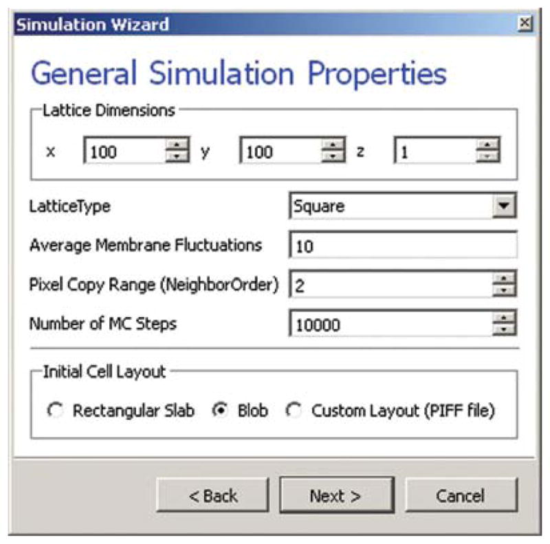
Specification of basic cell-sorting properties in Simulation Wizard. (For color version of this figure, the reader is referred to the web version of this book.)

In this example, we specify a 100 × 100 × 1 cell lattice, that is, a 2D model, a fluctuation amplitude of 10, a simulation duration of 10,000 MCS, and a pixel-copy range of 2. BlobInitializer initializes the simulation with a disk of cells of specified size.

On the next Wizard page (see Fig. 6), we name the cell types in the model. We will use two cell types: Condensing (more cohesive) and NonCondensing (less cohesive). CC3D by default includes a special generalized cell type, Medium, with unconstrained volume that fills otherwise unspecified space in the cell lattice.

Fig. 6.

Specification of cell-sorting cell types in Simulation Wizard. (For color version of this figure, the reader is referred to the web version of this book.)

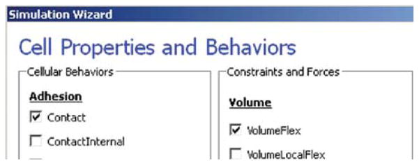
We skip the Chemical Field page of the Wizard and move to the Cell Behaviors and Properties page (see Fig. 7). Here, we select the biological behaviors we will include in our model. Objects in CC3D (for example, cells) have no properties or behaviors unless we specify then explicitly. Since cell sorting depends on differential adhesion between cells, we select the Contact Adhesion module from the Adhesion section (1) and give the cells a defined volume using the Volume Flex module from Constraints and Forces section.

Fig. 7.

Selection of cell-sorting cell behaviors in Simulation Wizard.² (For color version of this figure, the reader is referred to the web version of this book.)

We skip the next page related to Python scripting, after which Twedit++-CC3D generates the draft simulation code. Double-clicking on cellsorting.cc3d opens both the CC3DML (cellsorting.xml) and Python scripts for the model. Because the CC3DML file contains the complete model in this example, we postpone discussion of the Python script. A CC3DML file has three distinct sections. The first, the Lattice Section (lines 2–7) specifies global parameters like the cell-lattice size. The Plugin Section (lines 8–30) lists all the plugins used, for example, CellType and Contact. The Steppable Section (lines 32–39) lists all steppables; here we use only BlobInitializer.

All parameters appearing in the autogenerated CC3DML script have default values inserted by Simulation Wizard. We must edit the parameters in the draft CC3DML script to build a functional cell-sorting model (Listing 1). The CellType plugin (lines 9–13) already provides three generalized cell types: Condensing (C), NonCondensing (N), and Medium (M), so we need not change it.

Listing 1.

Simulation-Wizard-generated draft CC3DML (XML) code for cell sorting.³

However, the boundary-energy (contact energy) matrix in the Contact plugin (lines 22–30) is initially filled with identical values, which prevents sorting. For cell sorting, Condensing cells must adhere strongly to each other (so we set J_CC=2), Condensing and NonCondensing cells must adhere more weakly (here, we set J_CN=11), and all other adhesions must be very weak (we set J_NN=J_CM=J_NM=16), as discussed in Section III. The value of J_MM = 0 is irrelevant, since the Medium generalized cell does not contact itself.

To reduce artifacts due to the anisotropy of the square cell lattice we increase the neighbor order range in the contact energy to 2 so the contact energy sum in Eq. (1) will include nearest and second-nearest neighbors (line 29).

In the Volume plugin, which calculates the volume-constraint energy given in Eq. (1) the attributes CellType, LambdaVolume, and TargetVolume inside the <VolumeEnergyParameters> tags specify λ(τ) and V_t(τ) for each cell type. In our simulations, we set V_t(τ) = 25 and λ(τ) = 2.0 for both cell types.

We initialize the cell lattice using the BlobInitializer, which creates one or more disks (solid spheres in 3D) of cells. Each disk (sphere) created is enclosed between <Region> tags. The <Center> tag with syntax <Center x= “x_position” y= “y_position” z= “z_position”/> specifies the position of the center of the disk. The <Width> tag specifies the size of the initial square (cubical in 3D) generalized cells and the <Gap> tag creates space between neighboring cells. The <Types> tag lists the cell types to fill the disk. Here, we change the Radius in the draft BlobInitializer specification to 40. These few changes produce a working cell-sorting simulation.

To run the simulation, we right click cellsorting.cc3d in the left panel and choose the Open In Player option. We can also run the simulation by opening CompuCellPlayer and selecting cellsorting.cc3d from the File-> Open Simulation File dialog.

Fig. 8 shows snapshots of a simulation of the cell-sorting model. The less-cohesive NonCondensing cells engulf the more cohesive Condensing cells, which cluster and form a single central domain. By changing the boundary energies we can produce other cell-sorting patterns (Glazier and Graner, 1993; Graner and Glazier, 1992). In particular, if we reduce the contact energy between the Condensing cell type and the Medium, we can force inverted cell sorting, where the Condensing cells surround the NonCondensing cells. If we set the heterotypic contact energy to be less than either of the homotypic contact energies, the cells of the two types will mix rather than sort. If we set the cell-medium contact energy to be very small for one cell type, the cells of that type will disperse into the medium, as in cancer invasion. With minor modifications, we can also simulate the scenarios for three or more cell types, for situations in which the cells of a given type vary in volume, motility or adhesivity, or in which the initial condition contains coherent clusters of cells rather than randomly mixed cells (engulfment).

Fig. 8.

Snapshots of the cell-lattice configurations for the cell-sorting simulation in Listing 1. The boundary-energy hierarchy drives NonCondensing (light grey) cells to surround Condensing (dark grey) cells. The white background denotes surrounding Medium.

B. Angiogenesis Model

Vascular development is central to both development and cancer progression. We present a simplified model of the earliest phases of capillary network assembly by endothelial cells based on cell adhesion and contact-inhibited chemotaxis. This model does a good job of reproducing the patterning and dynamics which occur if we culture human umbilical vein endothelial cells (HUVEC) on matrigel in a quasi-2D in vitro experiment (Merks and Glazier, 2006; Merks et al., 2006, 2008). In addition to generalized cells modeling the HUVEC, we will need a diffusing chemical object, here, vascular endothelial growth factor (VEGF), cell secretion of VEGF, and cell-contact-inhibited chemotaxis to VEGF.

We will use a 3D voxel (pixel) with a side of 4 μm, that is, a volume of 64 μm³. Since the experimental HUVEC speed is about 0.4 μm/min and cells in this simulation move at an average speed of 0.1 pixel/MCS, one MCS represents 1 min.

In the Simulation Wizard, we name the model ANGIOGENESIS, set the cell- and field-lattice dimensions to 50 × 50 × 50, the membrane fluctuation amplitude to 20, the pixel-copy range to 3, the number of MCS to 10,000, and select BlobFieldInitializer to produce the initial cell-lattice configuration. We have only one cell type – Endothelial.

In the Chemical Fields page (see Fig. 9), we create the VEGF field and select FlexibleDiffusionSolverFE from the Solver pull-down list.

Fig. 9.

Specification of the angiogenesis chemical field in Simulation Wizard. (For color version of this figure, the reader is referred to the web version of this book.)

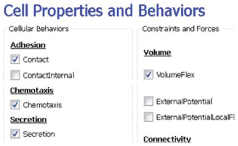
Next, on the CellPropertiesandBehaviors page (see Fig. 10), we select the Contact module from the Adhesion-behavior group and add Secretion, Chemotaxis, and Volume-constraint behaviors by checking the appropriate boxes.

Fig. 10.

Specification of angiogenesis cell behaviors in Simulation Wizard. (For color version of this figure, the reader is referred to the web version of this book.)

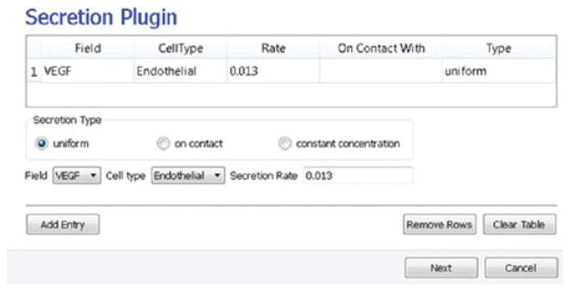
Because we have invoked Secretion and Chemotaxis, the Simulation Wizard opens their configuration screens. On the Secretion page (see Fig. 11), from the pull-down list, we select the chemical to secrete by selecting VEGF in the Field pull-down menu and the cell type secreting the chemical (Endothelial), and enter the rate of 0.013 (50 pg/(cell h) = 0.013 pg/(voxel MCS), compare to Leith and Michelson, 1995). We leave the Secretion Type entry set to Uniform, so each pixel of an endothelial cell secretes the same amount of VEGF at the same rate. Uniform volumetric secretion or secretion at the cell’s center of mass may be most appropriate in 2D simulations of planar geometries (e.g., cells on a petri dish or agar) where the biological cells are actually secreting up or down into a medium that carries the diffusant. CC3D also supplies a secrete-on-contact option to secrete outward from the cell boundaries and allows specification of which boundaries can secrete, which is more realistic in 3D. However, users are free to employ any of these methods in either 2D or 3D, depending on their interpretation of their specific biological situation. CC3D does not have intrinsic units for fields, so the amount of a chemical can be interpreted in units of moles, number of molecules, or grams. We click the Add Entry button to add the secretion information, then proceed to the next page to define the cells’ chemotaxis properties.

Fig. 11.

Specification of angiogenesis secretion parameters in Simulation Wizard. (For color version of this figure, the reader is referred to the web version of this book.)

On the Chemotaxis page, we select VEGF from the Field pull-down list and Endothelial for the cell type, entering a value for Lambda of 5000. When the chemotaxis type is regular, the cell’s response to the field is linear; that is the effective strength of chemotaxis depends on the product of Lambda and the secretion rate of VEGF, for example, a Lambda of 5000 and a secretion rate of 0.013 has the same effective chemotactic strength as a Lambda of 500 and a secretion rate of 0.13. Since endothelial cells do not chemotax at surfaces where they contact other endothelial cells (contact inhibition), we select Medium from the pull-down menu next to the Chemotax Towards button and click this button to add Medium to the list of generalized cell types whose interfaces with Endothelial cells support chemotaxis. We click the Add Entry button to add the chemotaxis information, then proceed to the final Simulation Wizard page Fig. 12.

Fig. 12.

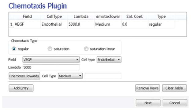
Specification of angiogenesis chemotaxis properties in Simulation Wizard. (For color version of this figure, the reader is referred to the web version of this book.)

Next, we adjust the parameters of the draft model. Pressure from chemotaxis to VEGF reduces the average endothelial cell volume by about 10 voxels from the target volume. So, in the Volume plugin, we set TargetVolume to 74 (64+10) and LambdaVolume to 20.0.

In experiments, in the absence of chemotaxis no capillary network forms and cells adhere to each other to form clusters. We therefore set J_MM=0, J_EM=12, and J_EE=5 in the Contact plugin (M: Medium, E: Endothelial). We also set the NeighborOrder for the Contact energy calculations to 4.

The diffusion equation that governs VEGF (V(x⃗)) field evolution is

$$\frac{\partial V(\overrightarrow{x})}{\partial t}=D_{\text{VEGF}}^{\text{EC}}{\nabla }^{2}V(\overrightarrow{x})-{\gamma }_{\text{VEGF}}V(\overrightarrow{x})\delta (\tau (\sigma (\overrightarrow{x})),M)+S^{\text{EC}}\delta (\tau (\sigma (\overrightarrow{x})),EC)$$ (3)

where δ(τ(σ(x⃗)), EC) = 1 inside Endothelial cells and 0 elsewhere and δ(τ(σ(x⃗)), M) = 1 inside Medium and 0 elsewhere. We set the diffusion constant D_VEGF = 0.042 μm²/s (0.16 voxel²/MCS, about two orders of magnitude smaller than experimental values),⁴ the decay coefficient γ_VEGF =1 h⁻¹ [130,131] (0.016 MCS⁻¹) for Medium pixels and γ_VEGF = 0 inside Endothelial cells, and the secretion rate S^EC = 0.013 pg/(voxel MCS).

In the CC3DML script, describing FlexibleDiffusionSolverFE (Listing 2, lines 38–47) we set the values of the <DiffusionConstant> and <DecayConstant> tags to 0.16 and 0.016, respectively. To prevent chemical decay inside endothelial cells, we add the line <DoNotDecayIn>Endothelial</DoNotDecayIn> inside the <DiffusionData> tag pair.

Listing 2.

CC3DML code for the angiogenesis model.

Finally, we edit BlobInitializer (lines 49–56) to start with a solid sphere 10 pixels in radius centered at x = 25, y = 25, z = 25 with initial cell width 4, as in Listing 2.

The main behavior that drives vascular patterning is contact-inhibited chemotaxis (Listing 2, lines 26–30). VEGF diffuses away from cells and decays in Medium, creating a steep concentration gradient at the interface between Endothelial cells and Medium. Because Endothelial cells chemotax up the concentration gradient only at the interface with Medium, the Endothelial cells at the surface of the cluster compress the cluster of cells into vascular branches and maintain branch integrity.

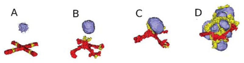
We show screenshots of a simulation of the angiogenesis model in Fig. 13 (Merks et al., 2008; Shirinifard et al., 2009). We can reproduce either 2D or 3D primary capillary network formation and the rearrangements of the network agree with experimentally observed dynamics. If we eliminate the contact inhibition, the cells do not form a branched structure (as observed in chick allantois experiments, Merks et al., 2008). We can also study the effects of surface tension, external growth factors, and changes in motility and diffusion constants on the pattern and its dynamics. However, this simple model does not include the strong junctions HUVEC cells make with each other at their ends after a period of prolonged contact. It also does not attempt to model the vacuolation and linking of vacuoles that leads to a connected network of tubes.

Fig. 13.

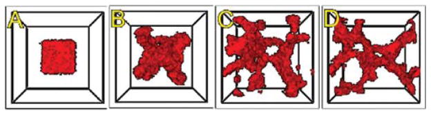
An initial cluster of adhering endothelial cells forms a capillary-like network via sprouting angiogenesis. (A) 0 h (0 MCS); (B) ~2 h (100 MCS); (C) ~5 h (250 MCS); (D): ~18 h (1100 MCS). (For color version of this figure, the reader is referred to the web version of this book.)

Since real endothelial cells are elongated, we can include the Cell-elongation plugin in the Simulation Wizard to better reproduce individual cell morphology. However, excessive cell elongation causes cell fragmentation. Adding either the Global or Fast Connectivity Constraint plugin prevents cell fragmentation.

C. Overview of Python Scripting in CompuCell3D

In the models we presented above, all cells had parameter values fixed in time. To allow cell behaviors to change, we need to be able to adjust cell properties during a simulation. CC3D can execute Python scripts (CC3D supports Python versions 2.x) to modify the properties of cells in response to events occurring during a simulation, such as the concentration of a nutrient dropping below a threshold level, a cell reaching a doubling volume, or a cell changing its neighbors. Most such Python scripts have a simple structure based on print statements, if-elif-else statements, for loops, lists, and simple classes and do not require in-depth knowledge of Python to create.

This section briefly introduces the main features of Python in the CC3D context. For a more formal introduction to Python, see Lutz (2011) and http://www.python.org.

Python defines blocks of code, such as those appearing inside if statements or for loops (in general after “:”), by an increased level of indentation. This chapter uses two spaces per indentation level. For example, in Listing 3, we indent the body of the if statement by two spaces and the body of the inner for loop by additional two spaces. The for loop is executed inside the if statement, which checks if we are in the second MCS of the simulation. The command pixelOffset=10 assigns to the variable pixelOffset a value of 10. The for loop assigns to the variable x values ranging from 0 through self.dim.x-1, where self.dim.x is a CC3D internal variable containing the size of the cell lattice in the x-direction. When executed, Listing 3 prints consecutive integers from 10 to 10+self.dim.x-1.

Listing 3.

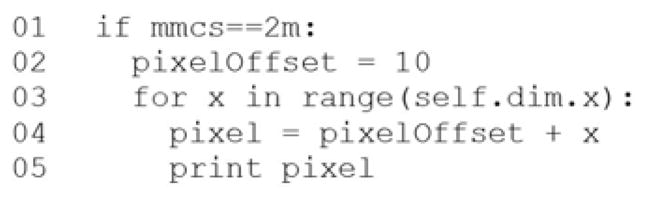
Simple Python loop.

One of the advantages of Python compared to older languages like Fortran is that it can also iterate over members of a Python list, a container for grouping objects. Listing 4 executes a for loop over a list containing all cells in the simulation and prints the type of each cell.

Listing 4.

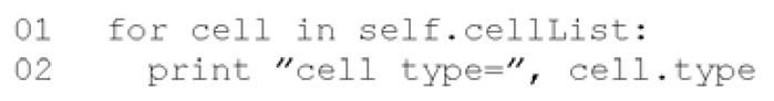
Iterating over the inventory of CC3D cells in Python.

Lists can combine objects of any type, including integers, strings, complex numbers, lists, and, in this case, CC3D cells. CC3D uses lists extensively to keep track of cells, cell neighbors, cell pixels, etc.

CC3D allows users to construct custom Python code as independent modules called steppables, which are represented as classes. Listing 5 shows a typical CC3D Python steppable class. The first line declares the class name together with an argument (SteppableBasePy) inside the parenthesis, which makes the main CC3D objects, including cells, lattice properties, etc., available inside the class. The def __init__(self,_simulator,_frequency=1): declares the initializing function __init__ which is called automatically during class object instantiation. After initializing the class and inheriting CC3D objects, we declare three main functions called at different times during the simulation: start is called before the simulation starts; step is called at specified intervals in MCS throughout the simulation; and finish is called at the end of the simulation. The start function iterates over all cells, setting their target volume and inverse compressibility to 25 and 5, respectively. Generically, we use the start function to define model initial conditions. The step function increases the target volumes of all cells by 0.001 after the tenth MCS, a typical way to implement cell growth in CC3D. The finish function prints the cell volumes at the end of the simulation.

Listing 5.

Sample CC3D steppable class.

The start, step, and finish functions have default implementations in the base class SteppableBasePy. Therefore, we only need to provide definition of those functions that we want to override. In addition, we can add our own functions to the class.

The next section uses Python scripting to build a complex CC3D model.

D. Three-Dimensional Vascular Tumor Growth Model

The development of a primary solid tumor starts from a single cell that proliferates in an inappropriate manner, dividing repeatedly to form a cluster of tumor cells. Nutrient and waste diffusion limits the diameter of such avascular tumor spheroids to about 1 mm. The central region of the growing spheroid becomes necrotic, with a surrounding layer of cells whose hypoxia triggers VEGF-mediated signaling events that initiate tumor neovascularization by promoting growth and extension (neoangiogenesis) of nearby blood vessels. Vascularized tumors are able to grow much larger than avascular spheroids and are more likely to metastasize.

Here, we present a simplified 3D model of a generic vascular tumor that can be easily extended to describe specific vascular tumor types and host tissues. We begin with a cluster of proliferating tumor cells, P, and normal vasculature. Initially, tumor cells proliferate as they take up diffusing glucose from the field, GLU, which the preexisting vasculature supplies (in this model, we neglect possible changes in concentration along the blood vessels in the direction of flow and set the secretion parameters uniformly over all blood-vessel surfaces). We assume that the tumor cells (both in the initial cluster and later) are always hypoxic and secrete a long-diffusing isoform of VEGF-A, L_VEGF. When GLU drops below a threshold, tumor cells become necrotic, gradually shrink and finally disappear. The initial tumor cluster grows and reaches a maximum diameter characteristic of an avascular tumor spheroid. To reduce execution time in our demonstration, we choose our model parameters so that the maximum spheroid diameter will be about 10 times smaller than in experiments. A few preselected neovascular endothelial cells, NV, in the preexisting vasculature respond both by chemotaxing toward higher concentrations of proangiogenic factors and by forming new blood vessels via neoangiogenesis. The tumor-induced vasculature increases the growth rate of the resulting vascularized solid tumor compared to an avascular tumor, allowing the tumor to grow beyond the spheroid’s maximum diameter. Despite our rescaling of the tumor size, the model produces a range of biologically reasonable morphologies that allow study of how tumor-induced angiogenesis affects the growth rate, size, and morphology of tumors.

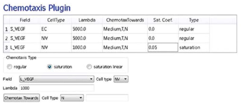
We use the basic angiogenesis simulation from the previous section to simulate both preexisting vasculature and tumor-induced angiogenesis, adding a set of finite-element links between the endothelial cells to model the strong junctions that form between endothelial cells in vivo. We denote the short-diffusing isoform of VEGF-A, S_VEGF. Both endothelial cells and neovascular endothelial cells chemotax up gradients of S_VEGF, but only neovascular endothelial cells chemotax up gradients of L_VEGF.

In the Simulation Wizard, we name the model TumorVascularization, set the cell- and field-lattice dimensions to 50 × 50 × 80, the membrane fluctuation amplitude to 20, the pixel-copy range to 3, the number of MCS to 10,000, and choose UniformInitializer to produce the initial tumor and vascular cells, since it automatically creates a mixture of cell types. We specify four cell types: P: proliferating tumor cells; N: necrotic cells; EC: endothelial cells; and NV: neovascular endothelial cells.

On the Chemical Fields page (see Fig. 14), we create the S_VEGF and L_VEGF fields and select FlexibleDiffusionSolverFE for both from the Solver pull-down list. We also check Enable multiple calls of PDE solvers to work around the numerical instabilities of the PDE solvers for large diffusion constants.

Fig. 14.

Specification of vascular tumor chemical fields in the Simulation Wizard. (For color version of this figure, the reader is referred to the web version of this book.)

On the Cell Behavior and Properties page (see Fig. 15) we select both the Contact and FocalPointPlasticity modules from the Adhesion group, and add Chemotaxis, Growth, and Mitosis, Volume Constraint, and GlobalConnectivity by checking the appropriate boxes. We also track the Center-of-Mass (to access field concentrations) and Cell Neighbors (to implement contact-inhibited growth). Unlike in our angiogenesis simulation, we will implement secretion as a part of the FlexibleDiffusionSolverFE syntax.

Fig. 15.

Specification of vascular tumor cell behaviors in Simulation Wizard. (For color version of this figure, the reader is referred to the web version of this book.)

In the Chemotaxis page (see Fig. 16), for each cell-type/chemical-field pair we click the Add Entry button to add the relevant chemotaxis information, for example, we select S_VEGF from the Field pull-down list and EC and NV from the cell-type list and set Lambda to 5000. To enable contact inhibition of EC and NV chemotaxis, we select Medium from the pull-down menu next to the Chemotax Towards button and click the button to add Medium to the list. We repeat this process for the T and N cell types, so that NV cells chemotax up gradients of L_VEGF. We then proceed to the final Simulation Wizard page.

Fig. 16.

Specification of vascular tumor chemotaxis properties in Simulation Wizard. (For color version of this figure, the reader is referred to the web version of this book.)

Twedit++ generates three simulation files – a CC3DML file specifying the energy terms, diffusion solvers, and initial cell layout, a main Python file that loads the CC3DMLfile, sets up the CompuCell environment and executes the Python steppables and a Python steppables file. The main Python file is typically constructed by modifying the standard template in Listing 6. Lines 1–12 set up the CC3D simulation environment and load the simulation. Lines 14–20 create instances of two steppables – MitosisSteppable and VolumeParamSteppable – and register them with the CC3D kernel. Line 22 starts the main CC3D loop, which executes MCSs and periodically calls the steppables.

Listing 6.

The Main Python script initializes the vascular tumor simulation and runs the main simulation loop.

Next, we edit the draft autogenerated simulation CC3DML file in Listing 7.

Listing 7.

CC3DML specification of the vascular tumor model’s initial cell layout, PDE solvers, and key cellular behaviors.

In Listing 7, in the Contact plugin (lines 36–53), we set J_MM=0, J_EM=12, and J_EE=5 (M: Medium, E: EC) and the NeighborOrder to 4. The FocalPointPlasticity plugin (lines 57–80) represents adhesion junctions by mechanically connecting the centers-of-mass of cells using a breakable linear spring (see Shirinifard et al., 2009). EC–EC links are stronger than EC–NV links, which are, in turn, stronger than NV–NV links (see the CC3D manual for details). Since the Simulation Wizard creates code to implement links between all cell-type pairs in the model, we must delete most of them, keeping only the links between EC–EC, EC–NV, and NV–NV cell types.

We assume that L_VEGF diffuses 10 times faster than S_VEGF, so D_{L_VEGF}=0.42 μm²/s (1.6 voxel²/MCS). This large diffusion constant would make the diffusion solver unstable. Therefore, in the CC3DML file (Listing 7, lines 108–114), we set the values of the <DiffusionConstant> and <DecayConstant> tags of the L_VEGF field to 0.16 and 0.0016, respectively, and use nine extra calls per MCS to achieve a diffusion constant equivalent to 1.6 (lines 87–89). We instruct P cells to secrete (line 116) into the L_VEGF field at a rate of 0.001 (3.85 pg/(cell h) = 0.001 pg/(voxel MCS)). Both EC and NV absorb L_VEGF. To simulate this uptake, we use the <SecretionData> tag pair (lines 117, 118).

Since the same diffusion solver will be called 10 times per MCS to solve S_VEGF, we must reduce the diffusion constant of S_VEGF by a factor of 10, setting the <DiffusionConstant> and <DecayConstant> tags of S_VEGF field to 0.016 and 0.0016, respectively. To prevent S_VEGF decay inside EC and NV cells, we add <DoNotDecayIn>EC</DoNotDecayIn> and <DoNotDecayIn>NV</DoNotDecayIn> inside the <DiffusionData> tag pair (lines 99, 100). We define S_VEGF to be secreted (lines 102–105) by both the EC and NV cells types at a rate of 0.013 per voxel per MCS (50 pg/(cell h) = 0.013 pg/(voxel MCS), compared to Leith and Michelson (1995).

The experimental glucose diffusion constant is about 600 μm²/s. We convert the glucose diffusion constant by multiplying by appropriate spatial and temporal conversion factors: 600 μm²/s × (voxel/4 μm)² × (60 s/MCS)=2250 voxel²/MCS. To keep our simulation times short for this example, we use a simulated glucose diffusion constant 1500 smaller, resulting in much steeper glucose gradients and smaller maximum tumor diameters. We could use the steady-state diffusion solver for the glucose field to be more realistic.

Experimental GLU uptake by P cells is ~0.3 μmol/g/min. We assume that stromal cells (represented here without individual cell boundaries by Medium) take up GLU at a slower rate of 0.1 μmol/g/min. A gram of tumor tissue has about 10⁸ tumor cells, so the glucose uptake per tumor cell is 0.003 pmol/MCS/cell or about 0.1 fmol/MCS/voxel. We assume that (at homeostasis) the preexisting vasculature supplies all the required GLU to Medium, which has a total mass of 1.28 × 10⁻⁵ grams and consumes GLU at a rate of 0.1 fmol/MCS/voxel, so the total GLU uptake (in the absence of a tumor) is 1.28 pmol/MCS. For this glucose to be supplied by 24 EC cells, their GLU secretion rate must be 0.8 fmol/MCS/voxel. We distribute the total GLU uptake (in the absence of a tumor) over all the Medium voxels, so the uptake rate is ~1.28 pmol/MCS/(~20,000 Medium voxels)=6.4 × 10⁻³ fmol/MCS/voxel.

We specify the uptake of GLU by Medium and P cells in lines 131 and 132 and instruct NV and EC cells to secrete GLU at the rate 0.4 and 0.8 pg/(voxel MCS), respectively (lines 129, 130).

We use UniformInitializer (lines 137–170) to initialize the tumor cell cluster and two crossing vascular cords. We also add two NV cells to each vascular cord, 25 pixels apart.

In the Python Steppable script in Listing 8, we set the initial target volume of both EC and NV cells to 74 (64 + 10) voxels and the initial target volume of tumor cells to 32 voxels (lines 14–21). All λ_vol are 20.0.

Listing 8.

Vascular tumor model Python steppables. The VolumeParametersSteppable adjusts the properties of the cells in response to simulation events and the MitosisSteppable implements cell division.

To model tumor cell growth, we increase the tumor cells’ target volumes (lines 38–47) according to:

$$\frac{{dV}_t(\text{tumor})}{dt}=\frac{G_{max}\mathit{GLU}(\overrightarrow{x})}{\mathit{GLU}(\overrightarrow{x})+{\mathit{GLU}}_0}$$ (4)

where GLU(x⃗) is the GLU concentration at the cell’s center-of-mass and GLU₀ is the concentration at which the growth rate is half its maximum. We assume that the fastest cell cycle time is 24 h, so G_max is 32 voxels/24 h = 0.022 voxel/MCS.

To account for contact-inhibited growth of NV cells, when their common surface area with other EC and NV cells is less than a threshold, we increase their target volume according to:

$$\frac{{dV}_t(NV)}{dt}=\frac{G_{max}L\_\mathit{VEGF}(\overrightarrow{x})}{L\_\mathit{VEGF}(\overrightarrow{x})+L\_{\mathit{VEGF}}_0}$$ (5)

where L_VEGF(x⃗) is the concentration of L_VEGF at the cell’s center-of-mass, L_VEGF₀ is the concentration at which the growth rate is half its maximum, and G_max is the maximum growth rate for NV cells. We calculate the common surface area between each NV cell and its neighboring NV or EC cells in lines 32–35. If the common surface area is smaller than 45, then we increase its target volume (lines 36, 37). When the volume of NVand P cells reaches a doubling volume (here, twice their initial target volumes), we divide them along a random axis, as shown in the MitosisSteppable (Listing 8, lines 54–75). The snapshots of the simulation are presented in Fig. 17

Fig. 17.

Two-dimensional snapshots of the vascular tumor simulation taken at: (A) 0 MCS; (B) 500 MCS; (C) 2000 MCS; (D) 5000 MCS. Red and yellow cells represent endothelial cells and neovascular endothelial cells, respectively. (See color plate.)

With this simple model we can easily explore the effects of changes in cell adhesion, nutrient availability, cell motility, sensitivity to starvation or dosing with chemotherapeutics or antiangiogenics on the growth and morphology of the simulated tumor.

E. Subcellular Simulations Using BionetSolver

While our vascular tumor model showed how to change cell-level parameters like target volume, we have not yet linked macroscopic cell behaviors to intracellular molecular concentrations. Signaling, regulatory, and metabolic pathways all steer the behaviors of biological cells by modulating their biochemical machinery. CC3D allows us to add and solve subcellular reaction-kinetic pathway models inside each generalized cell, specified using the SBML format (Hucka et al., 2003), and to use such models (e.g., of their levels of gene expression) to control cell-level behaviors like adhesion or growth (Hester et al., 2011).

We can use the same SBML framework to implement classic physics-based pharmacokinetic (PBPK) models of supercellular chemical flows between organs or tissues. The ability to explicitly model such subcellular and supercellular pathways adds greatly to the range of hypotheses CC3D models can represent and test. In addition, the original formulation of SBML primarily focused on the behaviors of biochemical networks within a single cell, whereas real signaling networks often involve the coupling of networks between cells. BionetSolver supports such coupling, allowing exploration of the very complex feedback resulting from intercell interactions linking intracellular networks, in an environment where the couplings change continuously due to cell growth, cell movement, and changes in cell properties.

As an example of such interaction between signaling networks and cell behaviors, we will develop a multi-cellular implementation of Delta–Notch mutual inhibitory coupling. In this juxtacrine signaling process, a cell’s level of membrane-bound Delta depends on its intracellular level of activated Notch, which in turn depends on the average level of membrane-bound Delta of its neighbors. In such a situation, the Delta–Notch dynamics of the cells in a tissue sheet will depend on the rate of cell rearrangement and the fluctuations it induces. Although the example does not explore the wide variety of tissue properties due to the coupling of subcellular networks with intercellular networks and cell behaviors, it already shows how different such behaviors can be from those of their non-spatial simplifications. We begin with the ODE Delta–Notch patterning model of Collier et al. (1996) in which juxtacrine signaling controls the internal levels of the cells’ Delta and Notch proteins. The base model neglects the complexity of the interaction due to changing spatial relationships in a real tissue:

$$\frac{dD}{dt}=v\left(\frac{1}{1+{bN}^h}-D\right)$$ (6)

$$\frac{dN}{dt}=\frac{{\overline{D}}^k}{a+{\overline{D}}^k}-N$$ (7)

where D and N are the concentrations of activated Delta and Notch proteins inside a cell, D̄ is the average concentration of activated Delta protein at the surface of the cell’s neighbors, a and b are saturation constants, h and k are Hill coefficients, and v is a constant that gives the relative lifetimes of Delta and Notch proteins.

Notch activity increases with the levels of Delta in neighboring cells, whereas Delta activity decreases with increasing Notch activity inside a cell (Fig. 18). When the parameters in the ODE model are chosen correctly, each cell assumes one of two exclusive states: a primary fate, in which the cell has a high level of Delta and a low level of Notch activity; and a secondary fate, in which the cell has a low level of Delta and a high level of Notch.

Fig. 18.

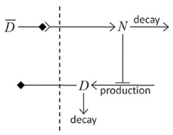
Diagram of Delta–Notch feedback regulation between and within cells.

To build this model in CC3D, we assign a separate copy of the ODE model (6–7) to each cell and allow each cell to see the Delta concentrations of its neighbors. We use CC3D’s BionetSolver library to manage and solve the ODEs, which are stored using the SBML standard.

The three files that specify the Delta–Notch model are included in the CC3D installation and can be found at <CC3D-installation-dir>/DemosBionetSolver/DeltaNotch: the main Python file (DeltaNotch.py) sets the parameters and initial conditions; the Python steppable file (DeltaNotch_Step.py) calls the subcellular models; and the SBML file (DN_Collier.sbml) contains the description of the ODE model. The first two files can be generated and edited using Twedit++, the last can be generated and edited using an SBML editor like Jarnac or JDesigner (both are open source). Listing 9 shows the SBML file viewed using Jarnac and can be downloaded from http://sys-bio.org.

Listing 9.

Jarnac specification of the Delta–Notch coupling model in Fig. 17.

The main Python file (DeltaNotch.py) includes lines to define a steppable class (DeltaNotchClass) to include the ODE model and its interactions with the CC3D generalized cells (Listing 10).

Listing 10.

Registering DeltaNotchClass in the main Python script, DeltaNotch.py in the Delta–Notch model.

The Python steppable file (Listing 11, DeltaNotch_Step.py) imports the BionetSolver library (line 1), then defines the class, and initializes the solver inside it (lines 2–5).

Listing 11.

Implementation of the _init_ and start functions of the DeltaNotchClass in the Delta–Notch model.

The first lines in the start function (Listing 11, lines 9–12) specify the name of the model, its nickname (for easier reference), the path to the location where the SBML model is stored, and the time-step of the ODE integrator, which fixes the relation between MCS and the time units of the ODE model (here, 1 MCS corresponds to 0.2 ODE model time units). In line 13, we use the defined names, path and time-step parameter to load the SBML model.

In Listing 11, line 15 associates the subcellular model with the CC3D cells, creating an instance of the ODE solver (described by the SBML model) for each cell of type TypeA. Line 16 initializes the loaded subcellular models.

To set the initial levels of Delta (D) and Notch (N) in each cell, we visit all cells and assign random initial concentrations between 0.9 and 1.0 (Listing 11, lines 18–26). Line 18 imports the intrinsic Python random number generator. Lines 22 and 23 pass these values to the subcellular models in each cell. The first argument specifies the ODE model parameter to change with a string containing the nickname of the model, here DN, followed by an underscore and the name of the parameter as defined in the SBML file. The second argument specifies the value to assign to the parameter, and the last argument specifies the cell id. For visualization purposes, we also store the values of D and N in a dictionary attached to each cell (lines 25, 26).

Listing 12 defines a step function of the class, which is called by every MCS, to read the Delta concentrations of each cell’s neighbors to determine the value of D (the average Delta concentration around the cell). The first three lines in Listing 12 iterate over all cells. Inside the loop, we first set the variables D and nn to zero. They will store the total Delta concentration of the cell’s neighbors and the number of neighbors, respectively. Next, we get a list of the cell’s neighbors and iterate over them. Line 9 reads the Delta concentration of each neighbor (the first argument is the name of the parameter and the second is the id of the neighboring cell) summing the total Delta and counting the number of neighbors. Note the += syntax (e.g., nn+=1 is equivalent to nn=nn+1). Lines 3 and 7 skip Medium (Medium has a value 0, so if (Medium) is false).

Listing 12.

Implementation of a step function (continuation of the code from Listing 11) to calculate D̄ in the DeltaNotchClass in the Delta–Notch model.

After looping over the cell’s neighbors, we update the variable D̄, which in the SBML code has the name Davg, to the average neighboring Delta (D) concentration, ensuing that the denominator, nn, is not zero (Listing 12, lines 10–12).

The remaining lines (Listing 12, lines 13–15) access the cell dictionary and store the cell’s current Delta and Notch concentrations. Line 16 then calls BionetSolver and tells it to integrate the ODE model with the new parameters for one integration step (0.2 time units in this case).

Fig. 19 shows a typical cell configurations and states for the simulation. The random initial values gradually converge to a pattern with cells with low levels of Notch (primary fate) surrounded by cells with high levels of Notch (secondary fate).

Fig. 19.

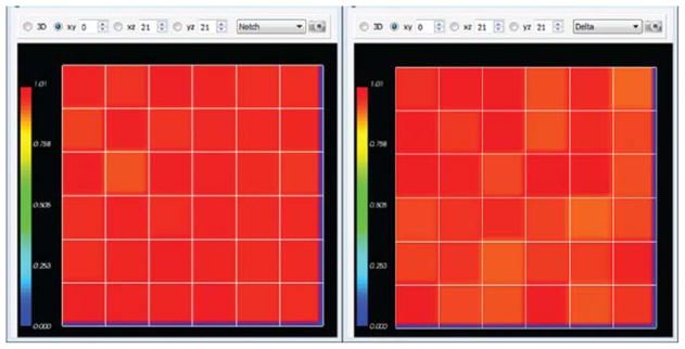
Initial Notch (left) and Delta (right) concentrations in the Delta–Notch model. (For color version of this figure, the reader is referred to the web version of this book.)

In Listing 13, lines 2–4 define two new visualization fields in the main Python file (DeltaNotch.py) to visualize the Delta and Notch concentrations in CompuCell Player. To fill the fields with the Delta and Notch concentrations, we call the steppable class, ExtraFields (Listing 13, lines 6–9). This code is very similar to our previous steppable calls, with the exception of line 8, which uses the function setScalarFields()to reference the visualization Fields.

Listing 13.

Adding extra visualization fields in the main Python script DeltaNotch.py in the Delta–Notch model.

In the steppable file (Listing 14, DeltaNotch_Step.py) we use setScalarFields() to set the variables self.scalarField1 and self. scalarField2 to point to the fields DeltaField and NotchField, respectively. Lines 10 and 11 of the step function clear the two fields using clearScalarValueCellLevel(). Line 12 loops over all cells, line 13 accesses a cell’s dictionary, and lines 14 and 15 use the D and N entries to fill in the respective visualization fields, where the first argument specifies the visualization field, the second the cell to be filled, and the third the value to use.

Listing 14.

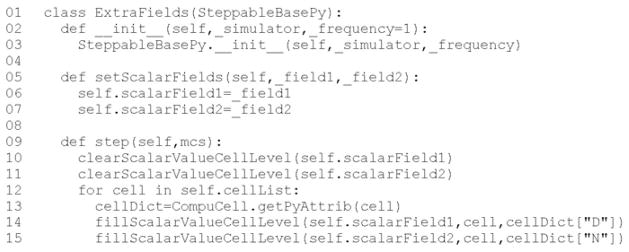
Steppable to visualize the concentrations of Delta and Notch in each cell in the Delta–Notch model.

The two fields can be visualized in CompuCell Player using the Field-selector button of the Main Graphics Window menu (second-to-last button, Fig. 19).

As we illustrate in Fig. 20, the result is a roughly hexagonal pattern of activity with one cell of low-Notch activity for every two cells with high Notch activity. In the presence of a high level of cell motility, the identity of high and low Notch cells can change when the pattern rearranges. We could easily explore the effects of Delta–Notch signaling on tissue structure by linking the Delta–Notch pathway to one of its known downstream targets. For example, if we wished to simulate embryonic feather-bud primordial in chicken skin or the formation of colonic crypts, we could start with an epithelial sheet of cells in 3D on a rigid support, and couple the growth of the cells to their level of Notch activity by having Notch inhibit cell growth. The result would be clusters of cell growth around the initial low-Notch cells, leading to a patterned 3D buckling of the epithelial tissue. Such mechanisms are capable of extremely complex and subtle patterning, as observed in vivo.

Fig. 20.

Dynamics of the Notch concentrations of cells in the Delta–Notch model. Snapshots taken at 10, 100, 300, 400, 450, and 600 MCS. (See color plate.)

V. Conclusion

Multi-cell modeling, especially when combined with subcell (or supercell) modeling of biochemical networks, allows the creation and testing of hypotheses concerning many key aspects of embryonic development, homeostasis, and developmental disease. Until now, such modeling has been out of reach to all but experienced software developers. CC3D makes the development of such models much easier, though it still does involve a minimal level of hand editing. We hope the examples we have shown will convince readers to evaluate the suitability of CC3D for their research.

Furthermore, CC3D directly addresses the current difficulty researchers face in reusing, testing, or adapting both their own and published models. Most published multi-cell, multi-scale models exist in the form of Fortran/C/C++ code, which is often of little practical value to other potential users. Reusing such code involves digging into large code bases, inferring their function, extracting the relevant code, and trying to paste it into a new context. CC3D improves this status quo in at least three ways: (1) it is fully open source; (2) CC3D models can be executed cross-platform and do not require compilation; (3) CC3D models are modular, compact, and shareable. Because Python-based CC3D models require much less effort to develop than does custom code programming: simulations are fast and easy to develop and refine. Even with these convenience features, CC3D 3.6 often runs as fast or faster than custom code solving the same model. Current CC3D development focuses on adding GPU-based PDE solvers, MPI parallelization, and additional cell behaviors. We are also developing a high-level cell-behavior model description language that will compile into executable Python, removing the last need for model builders to learn programming techniques.

All examples presented in this chapter are included in the CC3D binary distribution and will be curated to ensure their correctness and compatibility with future versions of CC3D.

References

- Alber MS, Jiang Y, Kiskowski MA. Lattice gas cellular automation model for rippling and aggregation in myxobacteria. Physica D. 2004;191:343–358. [Google Scholar]
- Alber MS, Kiskowski MA, Glazier JA, Jiang Y. On cellular automation approaches to modeling biological cells. In: Rosenthal J, Gilliam DS, editors. Mathematical Systems Theory in Biology, Communication and Finance. Springer-Verlag; New York: 2002. pp. 1–40. [Google Scholar]
- Alber M, Chen N, Glimm T, Lushnikov P. Multiscale dynamics of biological cells with chemotactic interactions: from a discrete stochastic model to a continuous description. Phys Rev E. 2006;73:051901. doi: 10.1103/PhysRevE.73.051901. [DOI] [PubMed] [Google Scholar]
- Armstrong PB, Armstrong MT. A role for fibronectin in cell sorting out. J Cell Sci. 1984;69:179–197. doi: 10.1242/jcs.69.1.179. [DOI] [PubMed] [Google Scholar]
- Armstrong PB, Parenti D. Cell sorting in the presence of cytochalasin B. J Cell Biol. 1972;55:542–553. doi: 10.1083/jcb.55.3.542. [DOI] [PMC free article] [PubMed] [Google Scholar]
- Chaturvedi R, Huang C, Izaguirre JA, Newman SA, Glazier JA, Alber MS. A hybrid discrete-continuum model for 3-D skeletogenesis of the vertebrate limb. Lect Notes Comput Sci. 2004;3305:543–552. [Google Scholar]
- Cickovski T, Aras K, Alber MS, Izaguirre JA, Swat M, Glazier JA, Merks RMH, Glimm T, Hentschel HGE, Newman SA. From genes to organisms via the cell: a problem-solving environment for multicellular development. Comput Sci Eng. 2007;9:50. doi: 10.1109/MCSE.2007.74. [DOI] [PMC free article] [PubMed] [Google Scholar]
- Cipra BA. An introduction to the Ising-model. Amer Math Monthly. 1987;94:937–959. [Google Scholar]
- Collier JR, Monk NAM, Maini PK, Lewis JH. Pattern formation by lateral inhibition with feedback: a mathematical model of Delta–Notch intercellular signaling. J Theor Biol. 1996;183:429–446. doi: 10.1006/jtbi.1996.0233. [DOI] [PubMed] [Google Scholar]
- Dallon J, Sherratt J, Maini PK, Ferguson M. Biological implications of a discrete mathematical model for collagen deposition and alignment in dermal wound repair. IMA J Math Appl Med Biol. 2000;17:379–393. [PubMed] [Google Scholar]
- Drasdo D, Kree R, McCaskill JS. Monte-Carlo approach to tissue-cell populations. Phys Rev E. 1995;52:6635–6657. doi: 10.1103/physreve.52.6635. [DOI] [PubMed] [Google Scholar]
- Glazier JA. Cellular patterns. Bussei Kenkyu. 1993;58:608–612. [Google Scholar]
- Glazier JA. Thermodynamics of cell sorting. Bussei Kenkyu. 1996;65:691–700. [Google Scholar]
- Glazier JA, Graner F. Simulation of biological cell sorting using a two-dimensional extended Potts model. Phys Rev Lett. 1992;69:2013–2016. doi: 10.1103/PhysRevLett.69.2013. [DOI] [PubMed] [Google Scholar]
- Glazier JA, Graner F. Simulation of the differential adhesion driven rearrangement of biological cells. Phys Rev E. 1993;47:2128–2154. doi: 10.1103/physreve.47.2128. [DOI] [PubMed] [Google Scholar]
- Glazier JA, Raphael RC, Graner F, Sawada Y. The energetics of cell sorting in three dimensions. In: Beysens D, Forgacs G, Gaill F, editors. Interplay of Genetic and Physical Processes in the Development of Biological Form. World Scientific Publishing Company; Singapore: 1995. pp. 54–66. [Google Scholar]
- Glazier JA, Balter A, Poplawski N. Magnetization to morphogenesis: a brief history of the Glazier–Graner–Hogeweg model. In: Anderson ARA, Chaplain MAJ, Rejniak KA, editors. Single-Cell-Based Models in Biology and Medicine. Birkhauser Verlag; Basel, Switzerland: 2007. pp. 79–106. [Google Scholar]
- Glazier JA, Zhang Y, Swat M, Zaitlen B, Schnell S. Coordinated action of N-CAM, N-cadherin, EphA4, and ephrinB2 translates genetic prepatterns into structure during somitogenesis in chick. Curr Top Dev Biol. 2008;81:205–247. doi: 10.1016/S0070-2153(07)81007-6. [DOI] [PMC free article] [PubMed] [Google Scholar]
- Graner F, Glazier JA. Simulation of biological cell sorting using a 2-dimensional extended Potts model. Phys Rev Lett. 1992;69:2013–2016. doi: 10.1103/PhysRevLett.69.2013. [DOI] [PubMed] [Google Scholar]
- Grieneisen VA, Xu J, Maree AFM, Hogeweg P, Schere B. Auxin transport is sufficient to generate a maximum and gradient guiding root growth. Nature. 2007;449:1008–1013. doi: 10.1038/nature06215. [DOI] [PubMed] [Google Scholar]
- Groenenboom MA, Hogeweg P. Space and the persistence of male-killing endosymbionts in insect populations. Proc Biol Sci. 2002;269:2509–2518. doi: 10.1098/rspb.2002.2197. [DOI] [PMC free article] [PubMed] [Google Scholar]
- Groenenboom MA, Maree AFM, Hogeweg P. The RNA silencing pathway: the bits and pieces that matter. PLoS Comput Biol. 2005;1:55–165. doi: 10.1371/journal.pcbi.0010021. [DOI] [PMC free article] [PubMed] [Google Scholar]
- Hester SD, Belmonte JM, Gens JS, Clendenon SG, Glazier JA. A Multi-cell, Multi-scale Model of Vertebrate Segmentation and Somite Formation. PLoS Comput Biol. 2011;7:e1002155. doi: 10.1371/journal.pcbi.1002155. [DOI] [PMC free article] [PubMed] [Google Scholar]
- Hogeweg P. Evolving mechanisms of morphogenesis: on the interplay between differential adhesion and cell differentiation. J Theor Biol. 2000;203:317–333. doi: 10.1006/jtbi.2000.1087. [DOI] [PubMed] [Google Scholar]
- Holm EA, Glazier JA, Srolovitz DJ, Grest GS. Effects of lattice anisotropy and temperature on domain growth in the two-dimensional Potts model. Phys Rev A. 1991;43:2662–2669. doi: 10.1103/physreva.43.2662. [DOI] [PubMed] [Google Scholar]
- Honda H, Mochizuki A. Formation and maintenance of distinctive cell patterns by coexpression of membrane-bound ligands and their receptors. Dev Dynamics. 2002;223:180–192. doi: 10.1002/dvdy.10042. [DOI] [PubMed] [Google Scholar]
- Hucka M, Finney A, Sauro HM, Bolouri H, Doyle JC, Kitano H, Arkin AP, Bornstein BJ, Bray D, Cornish-Bowden A, Cuellar AA, Dronov S, Gilles ED, Ginkel M, Gor V, Goryanin II, Hedley WJ, Hodgman TC, Hofmeyr J-H, Hunter PJ, Juty NS, Kasberger JL, Kremling A, Kummer U, Le Novère N, Loew LM, Lucio D, Mendes P, Minch E, Mjolsness ED, Nakayama Y, Nelson MR, Nielsen PF, Sakurada T, Schaff JC, Shapiro BE, Shimizu TS, Spence HD, Stelling J, Takahashi K, Tomita M, Wagner J, Wang J. The Systems biology markup language (SBML): a medium for representation and exchange of biochemical network models. Bioinformatics. 2003;19:524–531. doi: 10.1093/bioinformatics/btg015. [DOI] [PubMed] [Google Scholar]
- Johnston DA. Thin animals. J Phys A. 1998;31:9405–9417. [Google Scholar]
- Kesmir C, de Boer RJ. A spatial model of germinal center reactions: cellular adhesion based sorting of B cells results in efficient affinity maturation. J Theor Biol. 2003;222:9–22. doi: 10.1016/s0022-5193(03)00010-9. [DOI] [PubMed] [Google Scholar]
- Kesmir C, van Noort V, de Boer RJ, Hogeweg P. Bioinformatic analysis of functional differences between the immunoproteasome and the constitutive proteasome. Immunogenetics. 2003;55:437–449. doi: 10.1007/s00251-003-0585-6. [DOI] [PubMed] [Google Scholar]
- Knewitz MA, Mombach JCM. Computer simulation of the influence of cellular adhesion on the morphology of the interface between tissues of proliferating and quiescent cells. Comput Biol Med. 2006;36:59–69. doi: 10.1016/j.compbiomed.2004.08.002. [DOI] [PubMed] [Google Scholar]
- Leith JT, Michelson S. Secretion rates and levels of vascular endothelial growth factor in clone A or HCT-8 human colon tumour cells as a function of oxygen concentration. Cell Prolif. 1995;28:415–430. doi: 10.1111/j.1365-2184.1995.tb00082.x. [DOI] [PubMed] [Google Scholar]
- Longo D, Peirce SM, Skalak TC, Davidson L, Marsden M, Dzamba B. Multicellular computer simulation of morphogenesis: blastocoel roof thinning and matrix assembly in Xenopus laevis. Dev Biol. 2004;271:210–222. doi: 10.1016/j.ydbio.2004.03.021. [DOI] [PubMed] [Google Scholar]
- Lutz M. Programming Python. O’Reilly & Associates, Inc; Sebastopol, CA: 2011. [Google Scholar]
- Maini PK, Olsen L, Sherratt JA. Mathematical models for cell-matrix interactions during dermal wound healing. Int J Bifurcation Chaos. 2002;12:2021–2029. [Google Scholar]
- Marée AFM, Hogeweg P. How amoeboids self-organize into a fruiting body: multicellular coordination in Dictyostelium discoideum. Proc Natl Acad Sci USA. 2001;98:3879–3883. doi: 10.1073/pnas.061535198. [DOI] [PMC free article] [PubMed] [Google Scholar]
- Marée AFM, Hogeweg P. Modelling Dictyostelium discoideum morphogenesis: the culmination. Bull Math Biol. 2002;64:327–353. doi: 10.1006/bulm.2001.0277. [DOI] [PubMed] [Google Scholar]
- Marée AFM, Panfilov AV, Hogeweg P. Migration and thermotaxis of Dictyostelium discoideum slugs, a model study. J Theor Biol. 1999a;199:297–309. doi: 10.1006/jtbi.1999.0958. [DOI] [PubMed] [Google Scholar]
- Marée AFM, Panfilov AV, Hogeweg P. Phototaxis during the slug stage of Dictyostelium discoideum: a model study. Proc Royal Soc Lond Ser B. 1999b;266:1351–1360. [Google Scholar]
- Merks RM, Brodsky SV, Goligorksy MS, Newman SA, Glazier JA. Cell elongation is key to in silico replication of in vitro vasculogenesis and subsequent remodeling. Dev Biol. 2006;289:44–54. doi: 10.1016/j.ydbio.2005.10.003. [DOI] [PMC free article] [PubMed] [Google Scholar]
- Merks RM, Glazier JA. Dynamic mechanisms of blood vessel growth. Nonlinearity. 2006;19:C1–C10. doi: 10.1088/0951-7715/19/1/000. [DOI] [PMC free article] [PubMed] [Google Scholar]
- Merks RM, Perryn ED, Shirinifard A, Glazier JA. Contact-inhibited chemotactic motility can drive both vasculogenesis and sprouting angiogenesis. PLoS Comput Biol. 2008;4:e1000163. doi: 10.1371/journal.pcbi.1000163. [DOI] [PMC free article] [PubMed] [Google Scholar]
- Metropolis N, Rosenbluth A, Rosenbluth MN, Teller AH, Teller E. Equation of state calculations by fast computing machines. J Chem Phys. 1953;21:1087–1092. [Google Scholar]
- Meyer-Hermann M, Deutsch A, Or-Guil M. Recycling probability and dynamical properties of germinal center reactions. J Theor Biol. 2001;210:265–285. doi: 10.1006/jtbi.2001.2297. [DOI] [PubMed] [Google Scholar]
- Mochizuki A. Pattern formation of the cone mosaic in the zebrafish retina: A cell rearrangement model. J Theor Biol. 2002;215:345–361. doi: 10.1006/jtbi.2001.2508. [DOI] [PubMed] [Google Scholar]
- Mombach JCM, Glazier JA. Single cell motion in aggregates of embryonic cells. Phys Rev Lett. 1996;76:3032–3035. doi: 10.1103/PhysRevLett.76.3032. [DOI] [PubMed] [Google Scholar]
- Mombach JCM, de Almeida RMC, Thomas GL, Upadhyaya A, Glazier JA. Bursts and cavity formation in Hydra cells aggregates: experiments and simulations. Physica A. 2001;297:495–508. [Google Scholar]
- Mombach JCM, Glazier JA, Raphael RC, Zajac M. Quantitative comparison between differential adhesion models and cell sorting in the presence and absence of fluctuations. Phys Rev Lett. 1995;75:2244–2247. doi: 10.1103/PhysRevLett.75.2244. [DOI] [PubMed] [Google Scholar]
- Nguyen B, Upadhyaya A, van Oudenaarden A, Brenner MP. Elastic instability in growing yeast colonies. Biophys J. 2004;86:2740–2747. doi: 10.1016/S0006-3495(04)74327-1. [DOI] [PMC free article] [PubMed] [Google Scholar]
- Novak B, Toth A, Csikasz-Nagy A, Gyorffy B, Tyson JA, Nasmyth K. Finishing the cell cycle. J Theor Biol. 1999;199:223–233. doi: 10.1006/jtbi.1999.0956. [DOI] [PubMed] [Google Scholar]
- Popławski NJ, Shirinifard A, Swat M, Glazier JA. Simulation of single-species bacterial-biofilm growth using the Glazier–Graner–Hogeweg model and the CompuCell3D modeling environment. Math Biosci Eng. 2008;5:355–388. doi: 10.3934/mbe.2008.5.355. [DOI] [PMC free article] [PubMed] [Google Scholar]
- Popławski NJ, Swat M, Gens JS, Glazier JA. Adhesion between cells diffusion of growth factors and elasticity of the AER produce the paddle shape of the chick limb. Physica A. 2007;373:C521–C532. doi: 10.1016/j.physa.2006.05.028. [DOI] [PMC free article] [PubMed] [Google Scholar]
- Rieu JP, Upadhyaya A, Glazier JA, Ouchi NB, Sawada Y. Diffusion and deformations of single hydra cells in cellular aggregates. Biophys J. 2000;79:1903–1914. doi: 10.1016/S0006-3495(00)76440-X. [DOI] [PMC free article] [PubMed] [Google Scholar]
- Savill NJ, Hogeweg P. Modelling morphogenesis: from single cells to crawling slugs. J Theor Biol. 1997;184:229–235. doi: 10.1006/jtbi.1996.0237. [DOI] [PubMed] [Google Scholar]
- Savill NJ, Sherratt JA. Control of epidermal stem cell clusters by Notch-mediated lateral induction. Dev Biol. 2003;258:141–153. doi: 10.1016/s0012-1606(03)00107-6. [DOI] [PubMed] [Google Scholar]
- Steinberg MS. Differential adhesion in morphogenesis: a modern view. Curr Opin Genet Dev. 2007;17(4):281–286. doi: 10.1016/j.gde.2007.05.002. [DOI] [PubMed] [Google Scholar]
- Shirinifard A, Gens JS, Zaitlen BL, Poplawski NJ, Swat MH, Glazier JA. 3D multi-cell simulation of tumor growth and angiogenesis. PLoS ONE. 2009;4:e7190. doi: 10.1371/journal.pone.0007190. [DOI] [PMC free article] [PubMed] [Google Scholar]
- Takesue A, Mochizuki A, Iwasa Y. Cell-differentiation rules that generate regular mosaic patterns: modelling motivated by cone mosaic formation in fish retina. J Theor Biol. 1998;194:575–586. doi: 10.1006/jtbi.1998.0777. [DOI] [PubMed] [Google Scholar]
- Turner S, Sherratt JA. Intercellular adhesion and cancer invasion: a discrete simulation using the extended Potts model. J Theor Biol. 2002;216:85–100. doi: 10.1006/jtbi.2001.2522. [DOI] [PubMed] [Google Scholar]
- Walther T, Reinsch H, Grosse A, Ostermann K, Deutsch A, Bley T. Mathematical modeling of regulatory mechanisms in yeast colony development. J Theor Biol. 2004;229:327–338. doi: 10.1016/j.jtbi.2004.04.004. [DOI] [PubMed] [Google Scholar]
- Walther T, Reinsch H, Ostermann K, Deutsch A, Bley T. Coordinated growth of yeast colonies: experimental and mathematical analysis of possible regulatory mechanisms. Eng Life Sci. 2005;5:115–133. [Google Scholar]
- Wearing HJ, Owen MR, Sherratt JA. Mathematical modelling of juxtacrine patterning. Bull Math Biol. 2000;62:293–320. doi: 10.1006/bulm.1999.0152. [DOI] [PubMed] [Google Scholar]
- Zajac M. PhD thesis. University of Notre Dame; 2002. Modeling convergent extension by way of anisotropic differential adhesion. [Google Scholar]
- Zajac M, Jones GL, Glazier JA. Model of convergent extension in animal morphogenesis. Phys Rev Lett. 2000;85:2022–2025. doi: 10.1103/PhysRevLett.85.2022. [DOI] [PubMed] [Google Scholar]
- Zajac M, Jones GL, Glazier JA. Simulating convergent extension by way of anisotropic differential adhesion. J Theor Biol. 2003;222:247–259. doi: 10.1016/s0022-5193(03)00033-x. [DOI] [PubMed] [Google Scholar]
- Zhang Y, Thomas GL, Swat M, Shirinifard A, Glazier JA. Computer imulations of Cell Sorting Due to Differential Adhesion. PLoS ONE. 2011;6(10):e24999. doi: 10.1371/journal.pone.0024999. [DOI] [PMC free article] [PubMed] [Google Scholar]
- Zhdanov VP, Kasemo B. Simulation of the growth and differentiation of stem cells on a heterogeneous scaffold. Phys Chem Chem Phys. 2004a;6:4347–4350. [Google Scholar]
- Zhdanov VP, Kasemo B. Simulation of the growth of neurospheres. Europhys Lett. 2004b;68:134–140. [Google Scholar]