Accuracy of the Morphology Enabled Dipole Inversion (MEDI) Algorithm for Quantitative Susceptibility Mapping in MRI

Abstract

Determining the susceptibility distribution from the magnetic field measured in a magnetic resonance (MR) scanner is an ill-posed inverse problem, because of the presence of zeroes in the convolution kernel in the forward problem. An algorithm called morphology enabled dipole inversion (MEDI), which incorporates spatial prior information, has been proposed to generate a quantitative susceptibility map (QSM). The accuracy of QSM can be validated experimentally. However, there is not yet a rigorous mathematical demonstration of accuracy for a general regularized approach or for MEDI specifically. The error in the susceptibility map reconstructed by MEDI is expressed in terms of the acquisition noise and the error in the spatial prior information. A detailed analysis demonstrates that the error in the susceptibility map reconstructed by MEDI is bounded by a linear function of these two error sources. Numerical analysis confirms that the error of the susceptibility map reconstructed by MEDI is on the same order of the noise in the original MRI data, and comprehensive edge detection will lead to reduced model error in MEDI. Additional phantom validation and human brain imaging demonstrated the practicality of the MEDI method.

I. Introduction

Magnetic susceptibility is an important physical property of tissue, emerging as a new contrast mechanism in magnetic resonance imaging (MRI) [1]–[6]. The susceptibility of nonferromagnetic biomaterial generates a local field in the MR scanner, whose component along the main magnetic field is equal to the convolution of the volume susceptibility distribution with the magnetic field generated by a unit dipole, which will be referred to in the following as the unit dipole kernel. The convolution can be expressed as a pointwise multiplication of the susceptibility distribution and the unit dipole kernel in Fourier space for fast calculation [7]–[9]. The field is recorded in the MR signal phase. By solving the inverse problem, i.e., calculating the susceptibility source from the magnetic field, the tissue susceptibility can be determined quantitatively. However, because of the presence of zeroes at the magic angle (54.7) in the Fourier representation of the unit dipole kernel, a straightforward inversion would incur a division by zero, leading to meaningless susceptibility results.

A number of methods have been proposed to improve the stability of the inversion. The COSMOS [2], [4] method is model-free, but requires repeating the data acquisition at multiple orientations, severely limiting the practicality of this method. A single angle orientation reconstruction method is more practical but requires regularization in either Fourier space or image space. Several regularization methods have been investigated. Computationally, the simplest regularization may be the truncated k-space division method [3], [4] that works in k-space by selectively modifying the small values in the dipole kernel to avoid division by zero. Another weighted k-space division method [10] assumes that the susceptibility in Fourier domain is first-order differentiable and applies a modified L'Hospital's rule to interpolate susceptibility values near the magic angle. Computationally more complex regularization methods use spatial priors that assume the susceptibility distribution is smooth [11], sparse [11], or piece-wise constant [12]. Although these regularization methods are more practical than COSMOS in terms of using a single orientation data acquisition, there can be discrepancies between these mathematical models and the physical reality, causing errors in the susceptibility reconstruction. In general, these algorithmic biases have not been systematically analyzed and measured.

An advantage of MRI is its capability to simultaneously acquire structural and functional information. Previous experimental studies have shown that by properly incorporating additional morphological information from the MR magnitude image, the lack of measureable field data at the magic angle can be overcome, and a susceptibility map can be reconstructed with high quantitative accuracy [13], [14] in numerical simulations as well as in controlled experiments. The purpose of this work is to investigate the theoretical basis for this method, called morphology enabled dipole inversion (MEDI). Here we provide a detailed analytical and numerical investigation to demonstrate that this MEDI approach provides a unique and accurate solution under ideal conditions, and that the reconstruction error is tightly bounded by a linear function of the error in the gradient echo image in the presence of noise.

II. Theory

Accurate Solution in the Error-Free Case and Linearly Bounded Error in the General Case

In this section, we demonstrate that in the absence of noise and model error, the MEDI solution is unique and accurate, and we provide linear bounds for the worst-case reconstruction in the presence of error. Notations used in the following derivation are summarized in Table I.

TABLE I.

Notations

Symbol	Meaning
v	a column vector representation of a NxNyNz scalar field elements of v are denoted as voxels
∥ v ∥ p	Lp norm of v define as ${\left({\sum }_{i=1}^n{\mid v_i\mid }^p\right)}^{1∕p}$. p=2 if p is not specified
v’	a column vector representation of the gradient field of v containing 3NxNyNz elements elements of v’ are denoted as gradients
A	Matrix
AH	Hermitian transpose of A
A +	Moore-Penrose pseudo-inverse of A: A+ =(AH A)-1 AH
CS(A)	the column space of matrix A defined as the space spanned by the column vectors of A
ker(A)	The null space of matrix A defined as the space spanned by all vectors x fulfilling Ax=0
χ	General susceptibility distribution
χ 0	True susceptibility distribution
χ*	Estimated susceptibility distribution
δ φ	Local field
W	Data fidelity weighting matrix
FD	Matrix representation of dipole convolution
M	Edge weighting matrix
I	Identity matrix
ε	Expected noise level
zM	Number of diagonal zeros in M
λ	Regularization parameter

The original inverse problem of calculating the susceptibility χ from the measured local field δφ is formulated as a weighted least square minimization problem

$${\text{min}}_{\chi }{\Vert W(\delta \phi -F_D\chi )\Vert }_2$$ (1)

where W is a N × N (N being the number of voxels in χ) weighting matrix compensating for the nonuniform phase noise, which can be derived from the magnitude of the complex MRI data [11]; F_D is F_D = F^–1 DF with F being the 3-D Fourier transform; D is the Fourier domain representation of the unit dipole kernel and is a N × N diagonal matrix with diagonal elements equal to $1∕3-k_z^2∕k^2$, where k denotes the Fourier space coordinates and k_z denotes the Fourier space coordinate in the direction parallel to the main magnetic field. This minimization problem does not have a unique solution because F_D has a non-trivial null space, allowing different χ to generate a same local field.

In MEDI, the inverse problem is formulated as a constrained minimization problem by incorporating spatial priors

$${\text{min}}_{\chi }{\Vert M{\nabla }_{\chi }\Vert }_p,\mathrm{s}.\mathrm{t}.{\Vert W(\delta \phi -F_D\chi )\Vert }_2\le \epsilon .$$ (2)

Here, M is a 3N × 3N binary weighting diagonal matrix generated from the gradient of a morphological image such as the magnitude image by assigning zero to gradients representing substantial edges and one to all other gradients. Thus, M splits the gradients into two categories: edge gradients and nonedge gradients. Subscript p denotes L_p norm. ε is equal to the expected noise level.

If we denote χ’ = ∇χ, then the problem can be reformulated in terms of the susceptibility gradients:

$${\text{min}}_{{\chi }^{\prime }}{\Vert M{\chi }^{\prime }\Vert }_p,\mathrm{s}.\mathrm{t}.{\Vert W(\delta \phi -F_D{\nabla }^{+}{\chi }^{\prime })\Vert }_2\le \epsilon ,\text{curl}\left({\chi }^{\prime }\right)=0$$ (3)

where the constraint curl(χ’) = 0 is added to ensure that χ’ represents a gradient field. The true gradient field is denoted as ${\chi }_0^{\prime }$. The Helmholtz theorem states ∀χ’, curl(χ’) = 0 ⇔ χ’ ∈ CS(∇). The Moore–Penrose pseudo-inverse of ∇ is denoted ∇⁺ and it is determined at all points in the Fourier expression, except at the origin where it is set to zero, meaning the susceptibility map will be determined up to a constant.

We denote ${\Vert M{\chi }_0^{\prime }\Vert }_2$ as model error. The model error is expected to be small because the locations of most of the large elements in the true susceptibility gradients ${\chi }_0^{\prime }$ are expected to coincide with edge gradients in the morphological image as both kinds of edge arise from the same tissue interfaces. The model error is reducible by increasing z_M denoting the number of diagonal zeros in M, and ${\Vert M{\chi }_0^{\prime }\Vert }_2$ becomes zero when z_M = 3N. The observation $\delta \phi =F_D{\nabla }^{+}{\chi }_0^{\prime }+\mathit{e}$ is contaminated by noise e and the weighted L₂ norm of the noise is ∥We∥₂ = ε. The solution to (2) and (3) are respectively denoted as $\widehat{\chi }$ and ${\widehat{\chi }}^{\prime }$.

Lemma 1: The gradient reconstruction error ${\zeta }^{\prime }={\widehat{\chi }}^{\prime }-{\chi }_0^{\prime }$ satisfies ∥WF_D∇⁺ζ’∥₂ ≤ 2ε and ${\Vert M{\zeta }^{\prime }\Vert }_p<2{\Vert M{\chi }_0^{\prime }\Vert }_p$.

Proof: By applying variable substitution and the triangle inequality, we have

$${\Vert W{F}_D{\nabla }^{+}{\zeta }^{\prime }\Vert }_2={\Vert W(F_D{\nabla }^{+}{\widehat{\chi }}^{\prime }-F_D{\nabla }^{+}{\chi }_0^{\prime })\Vert }_2={\Vert W(F_D{\nabla }^{+}{\widehat{\chi }}^{\prime }-\delta \phi +\mathit{e})\Vert }_2\le {\Vert W(F_D{\nabla }^{+}{\widehat{\chi }}^{\prime }-\delta \phi )\Vert }_2+{\Vert W\mathit{e}\Vert }_2\le 2\epsilon .\therefore {\Vert W{F}_D{\nabla }^{+}{\zeta }^{\prime }\Vert }_2\le 2\epsilon$$

Because both ${\chi }_0^{\prime }$ and ${\widehat{\chi }}^{\prime }$ are in the feasible set of the constraint, and ${\widehat{\chi }}^{\prime }$ is also the solution to the minimization problem, ${\Vert M{\widehat{\chi }}^{\prime }\Vert }_p\le {\Vert M{\chi }_0^{\prime }\Vert }_p$. By applying variable substitution and the triangle inequality

$${\Vert M{\zeta }^{\prime }\Vert }_p={\Vert M{\widehat{\chi }}^{\prime }-M{\chi }_0^{\prime }\Vert }_p\le {\Vert M{\widehat{\chi }}^{\prime }\Vert }_p+{\Vert M{\chi }_0^{\prime }\Vert }_p\le 2{\Vert M{\chi }_0^{\prime }\Vert }_p\therefore {\Vert M{\zeta }^{\prime }\Vert }_p\le 2{\Vert M{\chi }_0^{\prime }\Vert }_p.$$

The use of spatial prior M allows the definition of a reduced problem in which the Euclidean distance between the measured local field and the field generated by edge gradients needs to be minimized

$${\text{min}}_{{\chi }^{\prime }\in \mathrm{CS}((I-M)\nabla )}{\Vert W(\delta \phi -F_D{\nabla }^{+}{\chi }^{\prime })\Vert }_2$$ (4)

where I is an identity matrix. If zero spatial prior is provided (M = 0), then the reduced problem is equivalent to the original ill-posed inverse problem in (1). This reduced problem has a unique solution if and only if the column space of (I – M)∇ only intersects with ker(WF_D∇⁺) at ζ’ = 0. Thus, we define the smallest eigenvalue of WF_D∇⁺ over the restricted subspace CS((I – M)∇) as

$$r_1={\text{min}}_{{\chi }^{\prime }\in \mathrm{CS}((I-M)\nabla ),{\chi }^{\prime }\ne 0}{\Vert \left(W{F}_D{\nabla }^{+}\right){\chi }^{\prime }\Vert }_2∕{\Vert {\chi }^{\prime }\Vert }_2.$$ (5)

The utility of these definitions will be clear in the following theorem proof. The condition for r₁ to be strictly positive is the same as the condition for the reduced problem to have a unique solution, i.e., the column space of (I – M)∇ only intersects with ker(WF_D∇⁺) at ζ’ = 0.

Theorem 1: If the reduced problem has a unique solution, then the solution to the original inverse problem of calculating susceptibility from magnetic field has bounded error. The norm of the error of the reconstructed susceptibility $\zeta =\widehat{\chi }-{\chi }_0$ is bounded by a linear function of the input error, which consists of the input model error defined as ${\Vert M{\chi }_0^{\prime }\Vert }_2$ and the input noise defined as ε. If additionally there is no input error, the solution is unique and accurate.

Proof: We decompose the gradient reconstruction error ζ’ into two parts: the error in the nonedge gradients or Mζ’ and those in the edge gradients or (I – M)ζ’. Note that ∥ζ’∥₂ = ∥(I – M + M)ζ’∥₂ ≤ ∥(I – M)ζ’∥₂ + ∥Mζ’∥₂, and that ${\Vert M{\zeta }^{\prime }\Vert }_2\le 2{\Vert M{\chi }_0^{\prime }\Vert }_2$ according to Lemma 1.

By applying the triangle inequality, we have

$${\Vert \left(W{F}_D{\nabla }^{+}\right)(I-M){\zeta }^{\prime }\Vert }_2\le {\Vert \left(W{F}_D{\nabla }^{+}\right){\zeta }^{\prime }\Vert }_2+{\Vert \left(W{F}_D{\nabla }^{+}\right)M{\zeta }^{\prime }\Vert }_2.$$

According to Lemma 1, we have ∥WF_D∇⁺)ζ’∥₂ ≤ 2ε. Additionally ∥WF_D∇⁺)Mζ’∥₂ is bounded by R∥Mζ’∥₂, where R is defined as

$$R={\text{max}}_{{\chi }^{\prime }\in \mathrm{CS}(M\nabla ),{\chi }^{\prime }\ne 0}{\Vert \left(W{F}_D{\nabla }^{+}\right){\chi }^{\prime }\Vert }_2∕{\Vert {\chi }^{\prime }\Vert }_2.\therefore {\Vert \left(W{F}_D{\nabla }^{+}\right)(I-M){\zeta }^{\prime }\Vert }_2\le 2\epsilon +R{\Vert M{\zeta }^{\prime }\Vert }_2\le 2(\epsilon +R{\Vert M{\chi }_0^{\prime }\Vert }_2).$$ (6)

Evoking the definition of r₁, r₁∥(I – M)ζ’∥₂ ≤ ∥WF_D∇⁺)(I – M)ζ’∥₂. If r₁ is strictly positive, the L₂ norm of the gradient error in the edge gradients has the following bound:

$${\Vert (I-M){\zeta }^{\prime }\Vert }_2\le 2(\epsilon +R{\Vert M{\chi }_0^{\prime }\Vert }_2)∕r_1.\therefore {\Vert {\zeta }^{\prime }\Vert }_2\le {\Vert (I-M){\zeta }^{\prime }\Vert }_2+{\Vert M{\zeta }^{\prime }\Vert }_2\le 2(\epsilon +R{\Vert M{\chi }_0^{\prime }\Vert }_2)∕r_1+2{\Vert M{\chi }_0^{\prime }\Vert }_2.$$

This shows that the error on the reconstructed gradient ${\widehat{\chi }}^{\prime }$ is linearly bounded by model error and noise. For the reconstructed susceptibility distribution $\widehat{\chi }$, if the constant term is omitted because only relative susceptibility is of interest, then the error ζ is also bounded by ∥ζ∥₂ ≤ ∥ζ’∥₂/r₂, where r₂ = min_{∇χ≠0,χ≠0}∥∇χ∥₂/∥χ∥₂ > 0. When the central difference is used for calculating the gradient, $r_2=\sqrt{{\text{sin}}^2(2\pi ∕N_x)+{\text{sin}}^2(2\pi ∕N_y)+{\text{sin}}^2(2\pi ∕N_z)}$, which only depends on image dimension N_x, N_y, N_z [15]. In the absence of input error, i.e., model error ${\Vert M{\chi }_0^{\prime }\Vert }_2=0$ and noise ε = 0, then ∥ζ∥₂ = 0, the solution is unique and accurate to the unknown susceptibility.

III. Materials and Methods

The theory section states that the norm of the reconstruction error ∥ζ∥ is bounded by

$$[2(\epsilon +R\Vert M{\chi }_0^{\prime }\Vert )∕r_1+2\Vert M{\chi }_0^{\prime }\Vert ]∕r_2=\epsilon \times 2∕\left(r_1{r}_2\right)+\Vert M{\chi }_0^{\prime }\Vert \times 2(R∕r_1+1)∕r_2.$$ (7)

To study the influence of image content and spatial prior information on the reconstruction error, a series of numerical simulations were carried out. Specifically, the relationship between and the error amplification bound, the effect of different regularization parameter and the error propagation due to noise or model error in the data.

A. Numerical Simulation

1) Numerical Phantom Construction

A numerical phantom was constructed consisting of cylinders, a sphere and a shell to mimic the geometry of common structures found in the human brain (Fig. 1). The image dimension was N_x × N_y × N_z voxels. The diameters of the cylinders, sphere and shell were chosen to be the smallest integer larger than N_x/32, N_x/12 and N_x/6, respectively. Uniform susceptibility values of 0.01, 0.02, and 0.05 ppm were assigned to the sphere, the shell, and the oblique cylinder, respectively. The susceptibility value in the horizontal cylinder linearly transitioned along its length from 0 to 0.04 ppm, and similarly from 0 to 0.03 ppm in the vertical cylinder. The range 0.01–0.05 ppm is representative of the range of susceptibilities found in the cortical gray matter and deep brain nuclei such as caudate nuclei or putamen in a young population [14]. A phase image was calculated using the forward equation based on the assumed susceptibility distribution [7]–[9]. Additionally, a corresponding magnitude image was also constructed using the same elements, with intensities 2, 1.3, and 1.6 for the lines, sphere, and shell, respectively. Complex zero mean Gaussian noise with a standard deviation, depending on the desired SNR of the lines, was added to the complex image formed by combining the phase and magnitude.

Fig. 1.

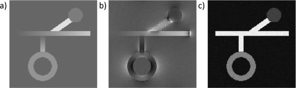
Numerical simulation phantom. Shown here are its (a) susceptibility distribution, (b) the corresponding phase, and (c) magnitude with SNR = 50 : 1.

2) Influence of M on the Error Bound

It is desirable to have a small 1/r₁ and a small R, both of which depend on the number of zeros on the diagonal of M, which has been denote by z_M. Therefore, we plotted the values of R, r₁, the noise amplification bound 2/(r₁r₂), and the model error amplification bound 2/r₂ · (R/r₁ + 1) against z_M. For a predetermined z_M, the weighting matrix M was determined as follows. The gradient of the magnitude images was calculated using the central difference. In an iterative process, a threshold was adjusted and applied to this gradient image by assigning zeroes to those voxels whose gradient is larger than the selected threshold. The iteration was stopped when the difference between number of zeroes thus obtained and the desired number of zeroes (z_M) was smaller than 5% of N = N_xN_yN_z,the total number of voxels in the original image. The resulting weighting matrix M was subsequently used for the calculation of R and r₁.

The value of R and r₁ in (5) and (6) can be found by calculating the largest and smallest eigenvalues over a restricted subspace, but this is different from the canonical definition of eigenvalue. Therefore, variable substitutions were performed to transform the problem. The calculation of r₁ is elaborated in the Appendix, and the same principle can be applied to calculate R. To ensure a finite bound exists, r₁ has to be strictly positive. This condition can be satisfied as long as the column space of (I – M)∇ does not intersect with the null space of WF_D∇⁺ anywhere besides 0. In this numerical analysis of the error bound, W was set to the identity matrix to simplify matters. Because the calculation of r₁ and R requires forming N × N matrices explicitly in memory, N_x = N_y = N_z = 16 with a corresponding r₂ = 0.66 was used for this section.

3) Influence of λ and M on the Image Quality

In this study, we chose p = 2 in the constrained minimization to demonstrate the propagation of the various error sources in the reconstruction. The solution of the constrained minimization problem in (2) reduced to an unconstrained Lagrangian problem with a properly chosen parameter λ

$${\chi }^{\ast }={\text{argmin}}_{\chi }({\Vert M\nabla \chi \Vert }_2^2+\lambda {\Vert W(\delta \phi -F_D\chi )\Vert }_2^2).$$ (8)

This inverse problem was then solved using a conjugate gradient method. A distribution χ = 0 was chosen as the initial solution, and the iteration stopped when the norm of the residual was less than 1% of the initial residual norm or when the number of iterations exceeded 200. The reconstruction was performed on a personal computer equipped with Intel core i7 and 8 GB of memory using MATLAB (MathWorks, Natick, MA). Reconstruction time was recorded, and the reconstruction error was measured by the L₂ norm of the difference between the reconstructed susceptibility map χ* and the known susceptibility map χ0. The discrepancy principle [16] was used to determine an optimal λ.

To investigate the effect of the edge weighting matrix M and regularization parameter _λ on the reconstruction quality (N_x = N_y = N_z = 64), we increased the number of zeroes in M or z_M linearly from 0.1 N to 1.3 N with a step size equal to 0.4 N, and varied λ from 10^–2 to 10² with a constant 2.31 multiplier. For a given M and l, reconstruction error was plotted against streaking artifact, which was calculated as the standard deviation of χ* in the background region where χ₀ = 0. This is essentially a 3-D extension of the 2-D measurement of streaking artifact proposed in [3]. Different _λs imposed different degrees of penalization of the spurious streaking artifacts often seen in susceptibility reconstructions. So streaking artifact, reconstruction error, and the norm of the residual of the data fidelity term normalized by the expected noise level ε were plotted against _λ. Imaging parameters commonly used in practice—B₀ = 3T and TE = 40 ms [14]—were used when simulating the phase image.

4) Influence of Noise and Model Error on the Reconstruction Error

To gauge the influence of acquisition noise ε on the reconstruction error, numerical phantoms (N_x = N_y = N_z = 64) were repeatedly generated with various SNR ranging from 5:1 to 95:1 with a step size of 10, from which the susceptibility distribution was estimated using the optimal _λ determined from the previous experiment and a perfect gradient weighting matrix ∥M₀∇χ₀∥ = 0. B₀ = 3T and TE = 40 ms were used when simulating the phase image. Reconstruction error was then plotted against ε.

To isolate the effect of model error on the reconstruction error, a second sphere with susceptibility equal to 0.04 ppm and radius equal to Nx/10 was added to χ₀ on a slice close to the existing structures such that it intersected with the original sphere. To simulate errors in the available edge information, the edge of the second sphere was gradually included in M from 0% (its edge was absent in M) to 100% (where the edge of the sphere was perfectly known in M). In addition, the edge of this second sphere was intentionally positioned on the wrong side of the existing sphere to further evaluate the influence of inaccurate edge information on the reconstruction. The acquisition noise level was set to zero in this simulation. B₀ = 3T and TE = 40 ms were used when simulating the phase image, and the optimal λ were used for the reconstruction. Reconstruction error was then plotted against ∥M∇χ₀∥.

B. Phantom Validation

A 2% agarose gel phantom containing five balloons of gadolinium solution (Magnevist, Berlex Labrotories, Wayne, NJ) was constructed. The highest concentration of the gadolinium was 0.5% followed by two-fold dilutions, leading to susceptibility values of 0.8, 0.4, 0.2, 0.1, and 0.05 ppm [12], [13]. This phantom was scanned on a 3T scanner (HDx, GE healthcare, Waukesha, WI) using a multi-echo gradient echo sequence with the following parameters: 8 TEs evenly spaced between 5 and 40 ms; TR = 70 ms; acquisition matrix = 130 × 130 × 86; voxel size = 1 × 1 × 1 mm³; flip angle = 15°; bandwidth = 480 Hz/pixel, scan time = 13 min.

The field map was estimated from the phase images across all the echoes on a voxel-by-voxel basis by performing a temporal phase unwrapping followed by a weighted linear least square fitting [11]. Frequency aliasing on the field map was resolved using a magnitude image guided spatial plane unwrapping algorithm. The background field caused by the phantom–air interface was removed through a projection onto dipole fields method [17] to obtain the local field map for inversion. Three susceptibility maps were generated, each using a different value for the parameter z_M : 3N (zero edge weighting), 0 (uniform edge weighting) and the optimal z_M determined from the numerical simulation. The regularization parameter λ used in each setting was determined iteratively using the discrepancy principle [16].

C. Human Brain Imaging

To illustrate that QSM is applicable to human brain imaging, we performed QSM on a healthy volunteer scanned on the same scanner using the same sequence as the phantom scan. This study was approved by our institutional review board. Imaging parameters were as follows: 11 TEs evenly spaced between 3 to 33 ms; TR = 37 ms; acquisition matrix = 240 × 240 × 150; voxel size = 1 × 1 × 1 mm³; flip angle = 15°; bandwidth = 520 Hz/pixel; a SENSE [18] based parallel imaging method, array spatial sensitivity encoding technique (ASSET), was enabled with a reduction factor of 2, resulting in a total scan time = 11min. The susceptibility map was reconstructed using the same method as described in the phantom section using z_M = 3N, z_M = 0 as well as the optimal z_M.

IV. Results

Fig. 2(a) shows that r₁ monotonically decreases from 0.04 to 0 as z_M (or the number of edge gradients) increases. It became zero at 1.53 N voxels. Fig. 2(b) shows that R is also monotonically decreasing from 1.8 to 1.0 over the same range but at a slower rate. Thus, the noise amplification bound, which is a function of 1/r₁, monotonically increased from 80 to 4596 when z_M increased from 0.04 to 1.53. Meanwhile, the model error amplification bound, which is dominated by the diminishing r₁, also increased from 143 to 5878.

Fig. 2.

Relationship between zeros in M(z_M) and the error bound in the reconstruction. a) r₁ decreases with increasing z_M. b) R gradually decreases with increasing z_M. c) Noise amplification bound increases with z_M. d) Model error amplification bound increases with z_M.

In Fig. 3, the global minimum was found at z_M = 0.9N and λ = 3.51. For different M or z_M, the local minima of reconstruction error consistently occurred at around λ ≈ 5. It was found that streaking artifact decreased with a decreasing λ, and that there was an optimal λ that led to the minimum reconstruction error. Additionally, for this value of λ, the residual of the solution matched the expected noise level. The reconstruction time was on average 50 s for each z_M and λ.

Fig. 3.

The influence of λ and M on streaking artifact and reconstruction error. a) For a given gradient weighting matrix M, the streaking artifact decreased as λ decreased while the reconstruction error showed a “V” shape pattern. For different z_M, the local minima of reconstruction error consistently occurred at around λ ≈ 5. b) The amount of streaking artifact monotonically decreased as λ decreased. c) An optimal λ was found at λ = 3.51 (circle) where the reconstruction error reached a minimum. d) The optimal λ also led to a solution whose residual matched the expected noise level.

Fig. 4(a)–(f) shows the susceptibility map reconstruction for two simulations with two different noise levels. When acquisition noise is the only source of error, the L₂ norm of the reconstruction error was linearly correlated with acquisition noise ε(r² = 0.997) and had a noise amplification factor 1.27 [slope = 1.27 in Fig. 3(e)], indicating the reconstruction error is on the same order of the input noise.

Fig. 4.

Relationship between noise and reconstruction error. When SNR = 15 : 1 and 95:1, the corresponding magnitude image (a and d), phase image (b and e), and reconstructed QSM (c and f) are shown. g) A linear relationship was observed between acquisition noise and reconstruction error.

Fig. 5(a)–(c) and (e)–(g) demonstrated that the streaking artifact gradually diminished as the edge information of the susceptibility source became more and more complete. In the case where the edge information is inaccurate, streaking artifact remained visible on the reconstruction [Fig. 5(d) and (h)]. In general, in the ideal case of zero noise ε = 0, reconstruction error was linearly correlated with model error $\Vert M{\chi }_0^{\prime }\Vert (r^2=0.998)$ and had a model error amplification factor 0.86 [slope = 0.86 in Fig. 5(k)], indicating the reconstruction error is on the same order of the model error.

Fig. 5.

Relationship between model error and reconstruction error. As the edge information of a sphere emerges from 0% (a), 50% (b) to 100% (c) in the gradient weighting M, the streaking artifact from the same sphere on the reconstructed QSM gradually diminishes (e–g). Erroneous edge information (d) does not necessarily lead to artificial susceptibility edges (h). i) A linear relationship was observed between model error and reconstruction error.

In the phantom result, the solution without edge weighting was severely corrupted by streaking artifact [Fig. 6(c)]. The solution with uniform edge weighting demonstrated blurring and residual streaking artifacts [Fig. 6(d)]. The solution with appropriate edge weighting showed suppressed streaking and well-delineated boundaries between gadolinium balloons and the background agarose gel [Fig. 6(e)]. The estimated susceptibility also showed the highest accuracy when compared to the prepared susceptibility. The reconstruction time was approximately 90 s for each z_M and λ.

Fig. 6.

Phantom experiment. Magnitude image is shown in a). The edge weighting derived from the predetermined optimal z_M = 0.9N is shown in (b) with gradients along x, y, z directions summed together for visualization. QSMs reconstructed using zero edge weighting (z_M = 3N) (c), uniform edge weighting (z_M = 0) (d), and magnitude derived edge weighting (z_M = 0.9N) (e) are shown. The solution (e) with magnitude-derived edge weighting (b) also led to the best quantitative accuracy (f).

In the human brain imaging, we observed similar patterns as in the phantom experiment. The solution without edge weighting [Fig. 7(d)] was severely corrupted by streaking artifact, while the solution with uniform edge weighting [Fig. 7(e)] demonstrated blurring and residual streaking artifacts. With appropriate edge weighting, the solution showed suppressed streaking and well-discernable deep brain nuclei such as the globus pallidus [arrow in Fig. 7(f)]. The reconstruction time was approximately 120 s for each z_M and λ.

Fig. 7.

Human brain QSM. Magnitude image from TE = 27 ms and the local field map are shown in a) and b). The edge weighting derived from the predetermined optimal z_M = 0.9N is shown in (c) with gradients along x, y, z directions summed together for visualization. QSMs reconstructed using zero edge weighting (z_M = 3N) (d), uniform edge weighting (z_M = 0) (e), and magnitude derived edge weighting (z_M = 0.9N) (f) are shown. Streaking artifacts seen in (d) and (e) are well-suppressed in (f). The arrow in f indicates the globus pallidus.

V. Discussion

In this study, an analysis was performed on the error of the susceptibility map estimated by the MEDI algorithm. It was found that this error was bounded by a linear function of both the acquisition noise and model error. This error propagation was confirmed in a simplified but representative numerical example. Specifically, in the absence of these sources of errors, the susceptibility solution is unique and accurate. The error analysis for various gradient weighting matrices M and regularization parameters λ may help to select the parameters for a robust MEDI reconstruction.

In the image reconstruction stage, the edge-weighting matrix M determines the type of regularization. It allows a trade-off between an unregularized solution and an over-regularized solution. When M is completely zero (z_M = 3N), the model error $\Vert M{\chi }_0^{\prime }\Vert$ is eliminated but the reconstruction error in this scenario is mathematically unbounded due to the lack of regularization and division by zero incurred at the magic angle. Severe streaking artifacts are usually seen in the unregularized solution [Fig.6(c) and Fig.7(d)]. When M is an identity matrix (z_M = 0), (8) is the conventional Tikhonov regularization applied on the gradient, which promotes global smoothness. With this regularization, streaking artifact is suppressed but at the expense of underestimating the true susceptibility contrast [Fig. 6(d) and (f)] because the algorithm cannot differentiate between these two types of signal variation. As a result, both residual streaking artifact and image smoothing may be observed simultaneously in the solution [Fig. 5(h), Fig. 6(d), and Fig. 7(e)]. However, when accurate edge information is provided on M, streaking artifact can be eliminated while preserving the susceptibility contrast [Fig. 5(g) and Fig. 6(e)]. The zeroes in M allow susceptibility changes at the edges without incurring any penalty to preserve the contrast. However, edge information does not necessarily create corresponding edges in the susceptibility distribution if the local field δφ indicates that no such susceptibility variations are present. In fact, the edge information provides a more realistic model for explaining observed data compared to Tikhonov regularization. Therefore, in our experiments, insufficient edge information resulted in residual streaking artifact [Fig. 5(b) and (f)], while a superfluous edge did not lead to artificial susceptibility contrast [Fig. 5(d) and (h)].

According to (7), to obtain a small bound on the total reconstruction error, it is desirable to have both a small model error $\Vert M{\chi }_0^{\prime }\Vert$ as well as a small 1/r₁ in the amplification bound, both of which depend on the number of edge gradients z_M. Thus, z_M provides a trade-off between model error and the amplification bound. Decreasing z_M will decrease the rank of (I – M) and reduce the range of (I – M)∇χ, where ∥(WF_D∇⁺)(I – M)∇χ∥/∥(I – M)∇χ∥ is minimized for calculating r₁. Accordingly, decreasing z_M will lead to a non-increasing amplification bound as demonstrated in Fig. 2(c) and (d), and z_M = 0 (uniform edge weighting) seems to be preferable. However, we empirically [Fig. 3(a) and Figs. 6 and 7] found that the final susceptibility error is less influenced by the error amplification bound 1/r₁ than the model error $\Vert M{\chi }_0^{\prime }\Vert$. For example in Fig. 6(c) and Fig. 7(d), although theoretically the error amplification was unbounded, which allows arbitrarily large error in the final reconstruction, the worst case (infinitely large error) was not reached in practice. Therefore, a relatively large z_M ≈ N proved to be beneficial because it led to the global optimum in our simulation [Fig. 3(a)], and also kept r₁ greater than zero to ensure a bounded error amplification. This choice z_M ≈ N is applicable to reconstructions of phantom (Fig. 6) and human data (Fig. 7), as well as demonstrated in another study [14]. For a typical 200 × 200 × 50 3-D human brain image with N = 2 × 10⁶ voxels, the number of edge gradients (the surface area of organ or lesion) is on the order of N^2/3(~ 1.6 × 10⁵), which is much smaller than N. Thus, the choice z_M = N may be sufficient to catch all tissue boundaries such that an adequate edge characterization and minimal model error becomes feasible. For this reason, a multiple echo MRI sequence is preferred for the data acquisition to allow a better edge detection: the magnitude contrast varies as the TE increases, decreasing the chances of missing edges when heterogeneous susceptibilities combined with accidental combinations of relaxation times T1, T2 and imaging parameters TR resulting in uniform signal.

In the theoretical derivation of the error bound, no assumption was made on the noise distribution, so the provided amplification factor 1/r₁ indicates the worst-case error amplification. When additive Gaussian noise is present on the complex image from a MRI acquisition and the image reflects physical objects, the reconstruction error increased almost linearly with the noise level in the phase image (Fig. 4) and the model error (Fig. 5). The linear relationship between reconstruction error and model acquisition noise suggests that a noise reduction in the MRI data will directly translate to a noise reduction in the reconstruction. Higher field strength and a longer echo time also contributes to the dephasing effect that provides a better contrast on the measured phase image. Although a single long TE often leads to signal loss due to T2* effect, which translates to higher phase noise, a multi-echo sampling strategy including early echoes can be used to circumvent this limitation [11].

In the theory section where the error bound was derived, we mainly used the triangle inequality for the derivation, which is a general property for norms. Therefore, the constraint in (2) may be formulated with an L₁ norm instead, and the same error bound derivation would still hold. Results in human brain imaging suggested that choosing p = 1 in the constraint is more effective than p = 2 in suppressing streaking artifacts [14], [19]. This may be explained by the theory that weighted L₁ norm minimization tends to sparsify the edges in the susceptibility map that do not correspond to edges in the magnitude image [20]. A systematic analysis is part of an ongoing research and is beyond the scope of this manuscript.

The optimal choice of the regularization parameter λ is an open question. When the regularization term is formulated in L ₂ norm, the choice of λ offers a trade-off between image piece-wise smoothness and data fidelity. We found that the discrepancy principle provides a reliable guideline for choosing λ, i.e., the residual of the data fidelity term produced by the final solution should match the expected noise level estimated from the MR image phase noise [Fig. 3(d)]. In practice, the choice of λ can be determined iteratively as implemented in a previous study [13]. Additionally, once the imaging acquisition protocol for a specific organ is established, it is our experience that the same λ can be applied across subjects due to the similarity in imaging content and noise level as shown in [14].

In this manuscript, we focused only on the error propagation in the dipole inversion stage. We acknowledge that the susceptibility measured using MRI is subject to various other error sources. Especially, image distortion, partial volume effect and finite resolution of the image may cause erroneous edge definition. In this study, experimental data were acquired with a multi-echo spoiled gradient echo sequence which is not susceptible to the potentially substantial geometric distortions seen with echo planar imaging. Partial volume effects and the point spread function indeed influenced the data, which can be seen on Fig. 6(a) and (b), where the edges of the balloons were generally wider than just 1 voxel. A wider edge introduced more zeros in the edge weighting M, reducing the model error and increasing the upper bound of model error amplification. However, it does not prevent the incorporation of the edge information in the MEDI algorithm. Fat signal is another challenge for imaging organs such as liver or breast. In this situation, water–fat separation techniques such as iterative decomposition of water and fat with echo asymmetry and least-squares estimation (IDEAL) [21] can be incorporated in the postprocessing to estimate the field map. From our experience and from the literature [4], [22], fat signal is a much smaller issue in the brain, which is a large area of focus for susceptibility mapping.

Image reconstruction constrained by spatial prior information was previously used in positron emission tomography (PET), electroencephalography (EEG), or magnetoencephalography (MEG) [23]–[25], where anatomical information from an additional high resolution MRI and CT was incorporated to localize signals. However, the source of structural information in MRI or CT is not directly related to the source of the detected signal in PET, EEG, or MEG. Consequently, MRI or CT structural constraints may have substantial model errors as investigated in Fig. 5. In the MEDI method, both morphology and field information are more fundamentally linked as they have the same physical origin, which includes the tissue susceptibility. They both naturally coexist as magnitude and phase in the complex MRI data, eliminating any spatial registration issue. This structural agreement between magnitude image and tissue susceptibility distribution provides a faithful spatial prior and accuracy for MEDI reconstructed susceptibility map.

VI. Conclusion

The error in a susceptibility reconstruction method using MEDI has two sources: data noise and error in the spatial prior. We demonstrated that 1) MEDI approach provides a unique and accurate solution under ideal conditions; 2) the error of the MEDI reconstructed susceptibility in general is bounded linearly by these two error sources; 3) when additive Gaussian noise is present on the complex image and the image reflects physical objects, the reconstruction error is on the same order of magnitude of the noise and the model error.

Appendix

The definition of r₁ is

$$r_1={\text{min}}_{{\chi }^{\prime }\in CS((I-M)\nabla ),{\chi }^{\prime }\ne 0}{\Vert \left(W{F}_D{\nabla }^{+}\right){\chi }^{\prime }\Vert }_2∕{\Vert {\chi }^{\prime }\Vert }_2.$$

By variable substitution

$${\chi }^{\prime }=(I-M)\nabla \chi ,A=W{F}_D{\nabla }^{+},B=(I-M)\nabla$$

we have

$$\begin{array}{cc}\hfill r_1& ={\text{min}}_{{\chi }^{\prime }\in \mathrm{CS}((I-M)\nabla ),{\chi }^{\prime }\ne 0}{\Vert \left(W{F}_D{\nabla }^{+}\right){\chi }^{\prime }\Vert }_2∕{\Vert {\chi }^{\prime }\Vert }_2\hfill \\ \hfill & ={\text{min}}_{\chi \in R^N,(I-M)\nabla \chi \ne 0}{\Vert \left(W{F}_D{\nabla }^{+}\right)\times (I-M)\nabla \chi \Vert }_2∕{\Vert (I-M)\nabla \chi \Vert }_2\hfill \\ \hfill & ={\text{min}}_{\chi \in R^N,B\chi \ne 0}{\Vert AB\chi \Vert }_2\hfill \\ \hfill & ={\text{min}}_{\chi \in R^N,B\chi \ne 0}\sqrt{{\chi }^H{\left(AB\right)}^{H}AB\chi ∕{\chi }^H{B}^{H}B\chi }\hfill \end{array}$$ (A1)

where A is N × 3N matrix, B is a 3N × N matrix and can be factorized using singular value decomposition B = UΣV^H with U being a 3N × 3N unitary matrix, Σ being a 3N × Ndiagonal matrix with nonnegative real diagonal number listed in descending order, and V being a N × N unitary matrix. If the rank of B is N_B, then the matrix Σ_NB formed by the first N_B columns of Σ has full rank.

We construct a matrix B_NB = UΣN B, then for any χ ∈ R^N, we can find a w ∈ R^N_B by taking the first N_B elements of V^Hχ, such that B _{N B}w = Bχ; for any w ∈ R^N_B, there is a χ = V[w0]^T ∈ R^N, such that Bχ = B _{N B}w. Therefore, the column space of $B_{NB}^H{B}_{NB}$ is identical to that of B ^H B, and $B_{NB}^H{B}_{NB}$ has full rank. With further variable substitution

$$\begin{array}{cc}\hfill r_1& ={\text{min}}_{\chi \in R^N,B\chi \ne 0}\sqrt{{\chi }^H{\left(AB\right)}^{H}AB\mathit{v}∕{\mathit{v}}^H{B}^{H}B\mathit{v}}\hfill \\ \hfill & ={\text{min}}_{w\in R^{N}B,\mathit{w}\ne 0}\sqrt{{\mathit{w}}^H{\left(A{B}_{NB}\right)}^{H}A{B}_{NB}\mathit{w}∕{\mathit{w}}^H{B}_{NB}^H{B}_{NB}\mathit{w}}.\hfill \end{array}$$ (A2)

The ratio expressed in (A2) is in form of the square root of a generalized Rayleigh quotient [26], whose minimum is the square root of the minimum generalized eigenvalue of (AB _{N B})^H AB _{N B} and $B_{NB}^H{B}_{NB}$. This can be calculated efficiently using generalized Schur decomposition [27].

References

- 1.Haacke EM, et al. Susceptibility weighted imaging (SWI) Magn. Reson. Med. 2004 Sep.52(3):612–618. doi: 10.1002/mrm.20198. [DOI] [PubMed] [Google Scholar]
- 2.Liu T, et al. Calculation of susceptibility through multiple orientation sampling (COSMOS): A method for conditioning the inverse problem from measured magnetic field map to susceptibility source image in MRI. Magn. Reson. Med. 2009 Jan.61(1):196–204. doi: 10.1002/mrm.21828. [DOI] [PubMed] [Google Scholar]
- 3.Shmueli K, et al. Magnetic susceptibility mapping of brain tissue in vivo using MRI phase data. Magn. Reson. Med. 2009 Dec.62(6):1510–22. doi: 10.1002/mrm.22135. [DOI] [PMC free article] [PubMed] [Google Scholar]
- 4.Wharton S, Schafer A, Bowtell R. Susceptibility mapping in the human brain using threshold-based k-space division. Magn. Reson. Med. 2010 May;63(5):1292–304. doi: 10.1002/mrm.22334. [DOI] [PubMed] [Google Scholar]
- 5.Liu C. Susceptibility tensor imaging. Magn. Reson. Med. 2010 Jun;63(6):1471–1477. doi: 10.1002/mrm.22482. [DOI] [PMC free article] [PubMed] [Google Scholar]
- 6.Haacke EM, et al. Susceptibility mapping as a means to visualize veins and quantify oxygen saturation. J. Magn. Reson. Imag. 2010 Sep.32(3):663–676. doi: 10.1002/jmri.22276. [DOI] [PMC free article] [PubMed] [Google Scholar]
- 7.Salomir R, De Senneville BD, Moonen CTW. A fast calculation method for magnetic field inhomogeneity due to an arbitrary distribution of bulk susceptibility. Concepts Magn. Reson. Part B—Magn. Reson. Eng. 2003 Oct.19B(1):26–34. [Google Scholar]
- 8.Marques JP, Bowtell R. Application of a Fourier-based method for rapid calculation of field inhomogeneity due to spatial variation of magnetic susceptibility. Concepts Magn. Reson. Part B: Magn. Reson. Eng. 2005;25B(1):65–78. [Google Scholar]
- 9.Koch KM, et al. Rapid calculations of susceptibility-induced magnetostatic field perturbations for in vivo magnetic resonance. Phys. Med. Biol. 2006 Dec.51(24):6381–6402. doi: 10.1088/0031-9155/51/24/007. [DOI] [PubMed] [Google Scholar]
- 10.Li W, Wu B, Liu C. Quantitative susceptibility mapping of human brain reflects spatial variation in tissue composition. Neuroimage. 2011 Apr.55(4):1645–1656. doi: 10.1016/j.neuroimage.2010.11.088. [DOI] [PMC free article] [PubMed] [Google Scholar]
- 11.Kressler B, et al. Nonlinear regularization for per voxel estimation of magnetic susceptibility distributions from MRI field maps. IEEE Trans. Med. Imag. 2010 Feb.29(2):273–281. doi: 10.1109/TMI.2009.2023787. [DOI] [PMC free article] [PubMed] [Google Scholar]
- 12.de Rochefort L, et al. Quantitative MR susceptibility mapping using piece-wise constant regularized inversion of the magnetic field. Magn. Reson. Med. 2008 Oct.60(4):1003–9. doi: 10.1002/mrm.21710. [DOI] [PubMed] [Google Scholar]
- 13.de Rochefort L, et al. Quantitative susceptibility map reconstruction from MR phase data using bayesian regularization: Validation and application to brain imaging. Magn. Reson. Med. 2010 Jan.63(1):194–206. doi: 10.1002/mrm.22187. [DOI] [PubMed] [Google Scholar]
- 14.Liu T, et al. Morphology enabled dipole inversion (MEDI) from a single-angle acquisition: Comparison with COSMOS in human brain imaging. Magn. Reson. Med. 2011 Sep.66(3):777–783. doi: 10.1002/mrm.22816. [DOI] [PubMed] [Google Scholar]
- 15.Gustafsson B, Kreiss H, Oliger J. Time Dependent Problems and Difference Methods. Wiley; New York: 1995. pp. 17–19. [Google Scholar]
- 16.Morozov VA. On the solution of functional equations by the method of regularization. Soviet. Math. Dokl. 1966;7:414–417. [Google Scholar]
- 17.Liu T, et al. A novel background field removal method for MRI using projection onto dipole fields (PDF) NMR Biomed. 2011 Nov.24(9):1129–36. doi: 10.1002/nbm.1670. [DOI] [PMC free article] [PubMed] [Google Scholar]
- 18.Pruessmann KP, et al. SENSE: Sensitivity encoding for fast MRI. Magn. Reson. Med. 1999 Nov.42(5):952–962. [PubMed] [Google Scholar]
- 19.Liu J, et al. Morphology enabled dipole inversion for quantitative susceptibility mapping using structural consistency between the magnitude image and the susceptibility map. Neuroimage. 2012 Feb.59(3):2560. doi: 10.1016/j.neuroimage.2011.08.082. [DOI] [PMC free article] [PubMed] [Google Scholar]
- 20.Candes EJ, Wakin MB, Boyd SP. Enhancing sparsity by reweighted l(1) minimization. J. Fourier Anal. Appl. 2008 Dec.14(5–6):877–905. [Google Scholar]
- 21.Reeder SB, et al. Multicoil dixon chemical species separation with an iterative least-squares estimation method. Magn. Reson. Med. 2004 Jan.51(1):35–45. doi: 10.1002/mrm.10675. [DOI] [PubMed] [Google Scholar]
- 22.Schweser F, et al. Quantitative imaging of intrinsic magnetic tissue properties using MRI signal phase: An approach to in vivo brain iron metabolism? Neuroimage. 2011 Feb.54(4):2789–807. doi: 10.1016/j.neuroimage.2010.10.070. [DOI] [PubMed] [Google Scholar]
- 23.Leahy R, Yan X. Information Processing in Medical Imaging . Vol. 511. Springer; New York: 1991. Incorporation of anatomical MR data for improved functional imaging with PET. LNCS. [Google Scholar]
- 24.Dale AM, Sereno MI. Improved localization of cortical activity by combining EEG and MEG with MRI cortical surface reconstruction—A linear-approach. J. Cognitive Neurosci. 1993 Spr.5(2):162–176. doi: 10.1162/jocn.1993.5.2.162. [DOI] [PubMed] [Google Scholar]
- 25.Beyer T, et al. A combined PET/CT scanner for clinical oncology. J. Nucl. Med. 2000 Aug.41(8):1369–1379. [PubMed] [Google Scholar]
- 26.Horn RA, Johnson CR. Matrix Analysis. Cambridge Univ. Press; Cambridge, U.K.: 1985. [Google Scholar]
- 27.Golub GH, Van Loan CF. Matrix Computations. 3rd ed. Johns Hopkins Univ. Press; Baltimore, MD: 1996. [Google Scholar]