Time-Frequency Mixed-Norm Estimates: Sparse M/EEG imaging with non-stationary source activations

Abstract

Magnetoencephalography (MEG) and electroencephalography (EEG) allow functional brain imaging with high temporal resolution. While solving the inverse problem independently at every time point can give an image of the active brain at every millisecond, such a procedure does not capitalize on the temporal dynamics of the signal. Linear inverse methods (Minimum-norm, dSPM, sLORETA, beamformers) typically assume that the signal is stationary: regularization parameter and data covariance are independent of time and the time varying signal-to-noise ratio (SNR). Other recently proposed non-linear inverse solvers promoting focal activations estimate the sources in both space and time while also assuming stationary sources during a time interval. However such an hypothesis only holds for short time intervals. To overcome this limitation, we propose time-frequency mixed-norm estimates (TF-MxNE), which use time-frequency analysis to regularize the ill-posed inverse problem. This method makes use of structured sparse priors defined in the time-frequency domain, offering more accurate estimates by capturing the non-stationary and transient nature of brain signals. State-of-the-art convex optimization procedures based on proximal operators are employed, allowing the derivation of a fast estimation algorithm. The accuracy of the TF-MxNE is compared to recently proposed inverse solvers with help of simulations and by analyzing publicly available MEG datasets.

1. Introduction

Distributed source models in magnetoencephalography and electroencephalography (collectively M/EEG) use thousands of current dipoles that are used as candidate sources to explain the M/EEG measurements. Those dipoles can be located on a dense three-dimensional grid within the brain volume, typically every 5 mm, or over a surface of the segmented cortical mantle [7], both of which can be automatically segmented from high-resolution anatomical Magnetic-Resonance Images (MRIs). Following Maxwell’s equations, each dipole adds its contribution linearly to the measured signal. Note that this linearity of the forward problem is not a modeling assumption but a fact based on the fundamental physics of the problem.

The task in the inverse problem is to map the M/EEG measurements to the brain, i.e., to estimate the distribution of dipolar currents that can explain the measured data. Inverse methods that estimate distributed sources are commonly referred to as imaging methods. This is motivated by the fact that the current estimate explains the data and can be visualized as an image, at least at a given point in time. The orientations of the dipoles can be either considered to be known, e.g., by aligning them with the estimated cortical surface normals [7], in which case only the dipole amplitudes need to be estimated. Alternatively, the orientations can be considered as unknown in which case both amplitudes and orientations need to be estimated at each spatial location.

One of the challenges for distributed inverse methods is that the number of dipoles by far exceeds the number of M/EEG sensors: the problem is ill-posed. Therefore, constraints using a priori knowledge based on the characteristics of the actual source distributions are necessary. Common priors are based on the Frobenius norm and lead to a family of methods generally referred to as mininum norm estimators (MNE) [45, 19]. Minimum norm estimates can be converted into statistical parameter maps, which take into account the noise level, leading to noise-normalized methods such as dSPM [6] or sLORETA [35]. While these methods have some benefits like simple implementation and a good robustness to noise, they do not take into account the natural assumption that only a few brain regions are typically active during a cognitive task. Interestingly, this latter assumption is what justifies a parametric method known as “dipole fitting” [37] routinely used in clinical practice. In order to promote such focal or sparse solutions within the distributed source model framework, one uses sparsity-inducing priors such as a ℓ_p norm with p ≤ 1 [30, 14]. However, with such priors it is challenging to obtain consistent estimates of the source orientations [42] as well as temporally coherent source estimates [34].

In order to promote spatio-temporally coherent focal estimates, several publications have proposed to constrain the active sources to remain the same over the time interval of interest [34, 11, 46, 15]. The implicit assumption is then that the sources are stationary. While this conjecture is reasonable for short time intervals, it is not a good model for realistic sources configurations where multiple transient sources activate sequentially during the analysis period, or simultaneously, before returning to baseline at different time instants.

When working with time series with transient and non-stationary effects, relevant signal processing tools are short time Fourier transforms (STFT) and wavelet decompositions. Contrary to a simple Fast Fourier Transform (FFT), they provide information localized in time and frequency (or scale). In particular, time-frequency decompositions, e.g., Morlet wavelet transforms, are routinely used in MEG and EEG analysis to study transient oscillatory signals. Such decompositions have been employed to analyze both sensor-level data and source estimates, but no attempt has been made to use their output in constructing a regularizer for the inverse problem.

In this contribution, we address the problem of localizing non-stationary focal sources from M/EEG data using appropriate sparsity inducing norms. Extending the work from [15] in which we coined the term Mixed-Norm Estimates (MxNE), we propose to use mixed-norms defined in terms of the time-frequency decompositions of the sources. We call this approach the Time-Frequency Mixed-Norms Estimates (TF-MxNE). The benefit is that the estimates can be obtained over longer time intervals while making standard preprocessing such as filtering or time-frequency analysis on the sensors optional. The inverse problem is formulated as in [15] as a convex optimization problem whose solutions are computed with an efficient solver based on proximal iterations.

We start with a detailed presentation of the problem and the algorithm. Next, we compare the characteristics and performance of various priors with help of realistic simulated data. Finally, we analyze publicly available MEG datasets (auditory and visual stimulations) demonstrating the benefit of TF-MxNE in terms of source localization and estimation of the time courses of the sources.

A preliminary version of this work was presented at the international conference on Information Processing in Medical Imaging (IPMI) [17]. In this paper we improve the solver to support loose orientation constraints, depth compensation as well as a debiasing step to better estimate source amplitudes. We also analyze new experimental data.

Notation: We indicate vectors with bold letters, a ∈ ℝ^N (resp. ) and matrices with capital bold letters, A ∈ ℝ^N×N (resp. ). a[i] stands for the i^th entry in the vector, while A[i, ·] and A[·, i] denote the i^th row and i^th column of a matrix, respectively. We denote ||A||_Fro the Frobenius norm, ${\left|\right|\mathbf{A}\left|\right|}_{\text{Fro}}^2={\sum }_{i,j=1}^N{\mid \mathbf{A}[i,j]\mid }^2,{\left|\right|\mathbf{A}\left|\right|}_1={\sum }_{i,j=1}^N\mid \mathbf{A}[i,j]\mid$ the ℓ₁ norm, and ${\left|\right|\mathbf{A}\left|\right|}_{21}={\sum }_{i=1}^N\sqrt{{\sum }_{j=1}^N{\mid \mathbf{A}[i,j]\mid }^2}$ the ℓ₂₁ mixed norm. A^T and A stand for the matrix transpose and a Hermitian transpose, respectively.

2. General model and method

After a short introduction to Gabor time-frequency dictionaries for M/EEG signals, we present the details of our TF-MxNE inverse problem approach. We then detail the proposed optimization strategy, which uses proximal iterations.

2.1. Gabor dictionaries

Here we briefly present some important properties of Gabor dictionaries, see [8] for more details. Given a signal observed over a time interval, its conventional Fourier transform estimates the frequency content but loses the time information. To analyze the evolution of the spectrum with time and hence the non-stationarity of the signal, Gabor introduced windowed Fourier atoms which correspond to a short-time Fourier transform (STFT) with a Gaussian window. In practice, for numerical computation, a challenge is to properly discretize the continuous STFT. The discrete STFT with a Gaussian window is also known as the discrete Gabor Transform [12].

The setting we are considering is the finite-dimensional one. Let g ∈ ℝ^T be a “mother” analysis window. Let f₀ ∈ ℕ and k₀ ∈ ℕ be the frequency and the time sampling rate in the time-frequency plane generated by the STFT, respectively. The family of the translations and modulations of the mother window generates a family of Gabor atoms (φ_mf)_mf forming the dictionary Φ ∈ , where K denotes the number of atoms. The atoms can be written as

$${\mathit{\phi }}_{mf}[n]=\mathbf{g}[n-{mk}_0]e^{\frac{i2\pi f_{0}fn}{T}},m\in \{0,\dots ,\frac{T}{k_0}-1\},f\in \{0,\dots ,\frac{T}{f_0}-1\}.$$ (1)

If the product f₀k₀ is small enough, i.e., the time-frequency plane is sufficiently sampled, the family (φ_mf)_mf is a frame of ℝ^T, i.e., one can recover any signal x ∈ ℝ^T from its Gabor coefficients (〈x, φ_mf 〉) = Φx. More precisely, there exists two constants A, B > 0 such that [1]:

$$A{\left|\right|\mathbf{x}\left|\right|}_2^2\le \sum _{m,f}{\mid \langle \mathbf{x},{\mathit{\phi }}_{mf}\rangle \mid }^2\le B{\left|\right|\mathbf{x}\left|\right|}_2^2.$$ (2)

When A = B, the frame is tight. When the vectors φ_mf are normalized the frame is an orthogonal basis if and only if A = B = 1. The Balian-Low theorem says that it is impossible to construct a Gabor frame which is a basis. Consequently, a Gabor transform is redundant or overcomplete and there exists an infinitely number of ways to reconstruct x from a given family of Gabor atoms. In the following, the considered Φ dictionaries are tight frames.

The canonical reconstruction of x from its Gabor coefficients requires a canonical dual window, denoted by g̃. Following (1) to define (φ̃_mf)_mf we have:

$$\mathbf{x}=\sum _{m,f}\langle \mathbf{x},{\mathit{\phi }}_{mf}\rangle {\stackrel{\sim }{\mathit{\phi }}}_{mf}=\sum _{m,f}\langle \mathbf{x},{\stackrel{\sim }{\mathit{\phi }}}_{mf}\rangle {\mathit{\phi }}_{mf}={\mathbf{\Phi }}^{\mathcal{H}}\mathbf{x}\stackrel{\sim }{\mathbf{\Phi }}={\stackrel{\sim }{\mathbf{\Phi }}}^{\mathcal{H}}\mathbf{x}\mathbf{\Phi },$$

where Φ̃ is the Gabor dictionary formed with the dual windows. When the frame is tight, then we have g̃ = g, and more particularly we have ΦΦ = ||ΦΦ||Id⁸. The representation being redundant, for any x ∈ ℝ^T one can find a set of coefficients z_mf such that x = Σ_m,f z_mfφ_mf, while the z_mf verify some suitable properties dictated by the application. For example, it is particularly interesting for M/EEG to find a sparse representation of the signal. Indeed, a scalogram, sometimes simply called TF transform of the data in the MEG literature, generally exhibits a few peaks localized in the time-frequency domain. In other words, an M/EEG signal can be expressed as a linear combinations of a few oscillatory atoms. In order to demonstrate this, Fig. 1 shows the STFT of a single planar gradiometer channel MEG signal from a somatosensory experiment, the same STFT restricted to the 50 largest coefficients (approximately only 10% of the coefficients), and the signal reconstructed with only these coefficients compared to the original signal. We observe that the true signal can be well approximated by only a few coefficients, i.e., a few Gabor atoms. In the presence of white Gaussian noise, restricting the time-frequency representation of a signal to the largest coefficients denoises the data. This stems from the fact, that Gaussian white noise in not sparse in the time-frequency domain, but rather spreads energy uniformly over all time-frequency coefficients [40]. Thresholding or shrinking the coefficients therefore reduces noise and smoothes the data. This is further explained in the context of wavelet transforms in [9].

Figure 1.

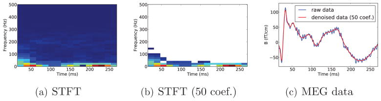
a) Short-time Fourier transform (STFT) of a single channel MEG signal sampled at 1000 Hz showing the sparse nature of the transformation (window size 64 time points and time shift k₀ = 16 samples). b) STFT restricted to the 50 largest coefficients c) Data and data reconstructed using only the 50 largest coefficients.

In practice, the Gabor coefficients are computed using the Fast Fourier Transform (FFT) and not by a multiplication by a Φ matrix as suggested above. Such operations can be efficiently implemented as in the LTFAT toolbox⁹ [38]. Another practical concern to keep in mind is the tradeoff between the size of the window g and the time shift k₀. A long window will have a good frequency resolution and a limited time resolution. The time resolution can be improved with a small time shift leading however to a larger computational cost, both in time and memory. Finally, as any computation done with an FFT, the STFT implementations assume circular boundary conditions for the signal. To take this into account and avoid edge artifacts, the signal has to be windowed, e.g., using a Hann window.

2.2. The inverse problem with time-frequency dictionaries

The linearity of Maxwell’s equations implies that the signals measured by M/EEG sensors are linear combinations of the electromagnetic fields produced by all current sources. The linear forward operator, called gain matrix, predicts the M/EEG measurements due to a configuration of sources based on a given volume conductor model [32]. Given such a linear forward operator G ∈ ℝ^N×P, where N is the number of sensors and P the number of sources, the measurements M ∈ ℝ^N×T (T number of time instants) are related to the source amplitudes X ∈ ℝ^P×T by M = GX.

The computation of the gain matrix G, e.g., with a Boundary Element Method (BEM) [24, 16], requires modeling of the electromagnetic properties of the head [19] such as the specification of the tissue conductivities. The matrix is then numerically computed. In the inverse problem one computes a best estimate of the neural currents, X^*, based on the measurements M. However, since P ≫ N, the problem is ill-posed and priors need to be imposed on X. Historically, the sources amplitudes were computed time instant by time instant using priors based on ℓ_p norms. The ℓ₂ (Frobenius) norm leads to MNE, LORETA, dSPM, or sLORETA while several alternative solvers based on ℓ_p norms with p ≤ 1 have also been proposed to promote sparse solutions [30, 14]. However, since such solvers work on an instant by instant basis they do not model the oscillatory nature of electromagnetic brain signals. Note that even if the ℓ₂ norm based methods work time instant by time instant, the estimates reflect the temporal characteristics of the data, since they are obtained by linear combinations of sensor data. This, however, implies that the parameters of the inverse solver are independent of time, which corresponds to assuming that the SNR is independent of time. Although MNE type approaches have been used with success, the assumption of constant SNR is clearly wrong since the signal amplitudes vary in time while the noise stays constant, or may be even smaller during an evoked response. The noise is usually estimated from baseline periods such as prestimulus intervals or periods when the brain is not yet responding to the stimulus.

Beyond single instant solvers, various sparsity-promoting approaches have been proposed [34, 11, 46]. Although they manage to capture the time courses of the activations more accuratly than the instantaneous sparse solvers, they implicitly assume that the active sources are the same over the entire time interval of interest. This also implies that if a source is detected as active at one time point, its activation will be non-zero during the entire time interval of interest. To go beyond this approach, we propose a solver which promotes on the one hand that the source configuration is spatially sparse, and on the other hand that the time course of each active dipole is a linear combination of a limited number of Gabor atoms, as suggested by Fig. 1. Since a Gabor oscillatory atom is localized in time, sources can be marked as active only during a short time period. The model reads:

$$\mathbf{M}=\mathbf{GX}+\mathbf{E}=\mathbf{GS}{\mathbf{\Phi }}^{\mathcal{H}}+\mathbf{E},$$ (3)

where Φ ∈ is a dictionary of K Gabor atoms, Z ∈ are the coefficients of the decomposition, and E is additive white noise, E ~ (0, λI). Given a prior on Z, (Z) ~ exp(−Ω(Z)), the maximum a posteriori estimate (MAP) is obtained by solving:

$${\mathbf{Z}}^{★}=\underset{\mathbf{Z}}{argmin}\frac{1}{2}{\left|\right|\mathbf{M}-\mathbf{GZ}{\mathbf{\Phi }}^{\mathcal{H}}\left|\right|}_{\text{Fro}}^2+\lambda \mathrm{\Omega }(\mathbf{Z}),\lambda >0.$$ (4)

If we consider Ω(Z) = ||Z||₁, (4) corresponds to a LASSO problem [39], a.k.a. Basis Pursuit Denoising (BPDN) [4], where features (or regressors) are spatio-temporal atoms. Similarly to the original formulation of MCE, i.e., ℓ₁ regularization without applying Φ, such a prior is likely to suffer from inconsistencies over time [34]. Indeed such a norm does not impose a structure for the non-zero coefficients: they are likely to be scattered all over Z^* (see Fig. 2). Therefore, simple ℓ₁ priors do not guarantee that only a few sources are active during the time window of interest. To promote this, one needs to employ mixed-norms such as the ℓ₂₁ norm [34, 15]. By doing so, the estimates have a sparse row structure (see Fig. 2). However the ℓ₂₁ prior on Z does not produce denoised time series as it does not promote source estimates that are formed by a sum of a few Gabor atoms. In order to recover the sparse row structure, while simultaneously promoting sparsity of the decompositions, we propose to use a composite prior formed by the sum of ℓ₂₁ and ℓ₁ norms. The prior then reads:

$$\lambda \mathrm{\Omega }(\mathbf{Z})={\lambda }_{\text{space}}{\left|\right|\mathbf{Z}\left|\right|}_{21}+{\lambda }_{\text{time}}{\left|\right|\mathbf{Z}\left|\right|}_1,{\lambda }_{\text{space}}>0,{\lambda }_{\text{time}}>0.$$ (5)

Figure 2.

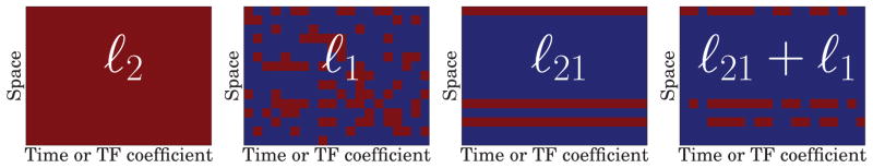
Sparsity patterns promoted by the different priors: ℓ₂ all non-zero, ℓ₁ scattered and unstructured non-zero, ℓ₂₁ block row structure, and ℓ₂₁ + ℓ₁ block row structure with intra-row sparsity. Red color indicates non-zero coefficients.

A large regularization parameter λ_space will lead to a spatially very sparse solution, while a large regularization parameter λ_time will promote sources with smooth times series. This is due to the uniform spectrum of the noise (see Section 2.1) and the fact that a large λ_time will promote source activations made up of few TF atoms, each of which has a smooth waveform.

2.3. Optimization strategy

The optimization strategy, which we propose for minimizing the cost function in (4), is based on the Fast Iterative Shrinkage Thresholding Algorithm (FISTA) [2], a first-order schemes that handles the minimization of any cost function that can be written as a sum of two terms: a smooth convex term f₁ with Lipschitz gradient and a convex term f₂, potentially non-differentiable: (Z) = f₁(Z) + f₂(Z). In order to apply FISTA, we need to be able to compute the so-called proximity operator associated with f₂, i.e., the proximity operator associated with the composite ℓ₂₁ + ℓ₁ prior [17].

Definition 1 (Proximity operator)

Let ϕ: ℝ^M → ℝ be a proper convex function. The proximity operator associated to ϕ, denoted by prox_ϕ: ℝ^M → ℝ^M reads:

$${\text{prox}}_{\varphi }(\mathbf{Z})=\underset{\mathbf{V}\in {\mathbb{R}}^M}{argmin}\frac{1}{2}{\left|\right|\mathbf{Z}-\mathbf{V}\left|\right|}_2^2+\varphi (\mathbf{V}).$$

While the proximity operators of mixed-norms relevant for M/EEG can be found in [15], in the case of the composite prior in (5), the proximity operator is given by the following lemma.

Lemma 1 (Proximity operator for ℓ₂₁ + ℓ₁)

Let Y ∈ be indexed by a double index (p, k). Z = prox_{λ||·||1+μ||·||21})(Y) ∈ is given for each coordinates (p, k) by

$$Z[p,k]=\frac{Y[p,k]}{\mid Y[p,k]\mid }{(\mid Y[p,k]\mid -\lambda )}_{+}{\left(1-\frac{\mu }{\sqrt{{\sum }_k{(\mid Y[p,k]\mid -\lambda )}_{+}^2}}\right)}_{+}.$$

where for x ∈ ℝ, (x)₊ = max(x 0), and by convention $\frac{0}{0}=0$.

This result is a corollary of the proximity operator derived for hierarchical group penalties recently proposed in [23]. The penalty described here can indeed be seen as a 2-level hierarchical structure, and the resulting proximity operator reduces to successively applying the ℓ₁ and ℓ₂₁ proximity operator. Both of these proximity operators are discussed in detail in [15].

The pseudo code is provided in Algorithm 1. The Lipschitz constant of the gradient of the smooth term in (4) is given by the square of the spectral norm of the linear operator Z → GZΦ. We estimate it with the power iteration method.

Algorithm 1.

FISTA with TF dictionaries to minimize 4

Input: Measurements M, gain matrix G, regularization parameter λ > 0 and I the number of iterations.
Output: Z*
1:	Auxiliary variables: Y and Zo ∈ ℝP×K, and τ and τo ∈ ℝ.
2:	Estimate the Lipschitz constant with the power iteration method.
3:	Y = Z* = Z, τ = 1, 0< μ <
4:	for i = 1 to I do
5:	Zo = Z*
6:	Z* = proxμλΩ(Y + μGT(M − GYΦ)Φ)
7:	τo = τ
8:	$\tau =\frac{1+\sqrt{1+4{\tau }^2}}{2}$
9:	$\mathbf{Y}={\mathbf{Z}}^{★}+\frac{{\tau }_o-1}{\tau }({\mathbf{Z}}^{★}-{\mathbf{Z}}_o)$
10:	end for

3. Specific modeling for M/EEG inverse problem

The M/EEG literature has shown that general solvers of the statistics literature need to be adapted to the specificities of the M/EEG inverse problem. Crucial steps in the computation of the source estimates are noise whitening, depth compensation, handling of source orientations, and amplitude bias correction.

3.1. Spatial whitening

The model in (3) assumes that the additive noise is Gaussian white with E ~ (0, λI). This strong modeling assumption is made realistic by a whitening step that relies on estimating the noise covariance matrix. For this purpose, baseline data is employed, which is recorded while the subject is at rest e.g. during pre-stimulus periods. If only MEG is recorded, the noise covariance can be estimated from data recorded without subject, often called empty room data. This approach provides good estimates of the measurement noise level. Although the noise level depends on the signal frequency, one usually uses a single frequency-unspecific noise covariance matrix. An alternative approach for frequency-dependent spatial whitening is presented in [36].

The whitening step is particularly fundamental when different sensor types are used: EEG and MEG with gradiometers and magnetometers record signals with different units of measure and with different noise levels. The whitening step makes data recorded by different sensors comparable and adapted for joint estimation.

3.2. Source models with unconstrained orientations

When the source orientations given by the normals of the cortical mesh cannot be trusted, it can be interesting to relax this constraint by placing three orthogonal sources at each spatial location. When all three orientations are allowed to explain the data equivalently the model is called free orientation. Moreover, it can be of interest to have intermediate models using loose orientation constraints [27]. However for such loose and free orientation models, the TF composite prior needs to be adapted. Let each source be indexed by a spatial location i and an orientation o ∈ {1, 2, 3}. Let o = 1 correspond to the orientation normal to the cortex, and o = 2 and o = 3 the two tangential orientations. We call 0 < ρ ≤ 1, the parameter controlling how loose is the orientation constraint. The ℓ₁ and ℓ₂₁ norms read:

$${\left|\right|\mathbf{Z}\left|\right|}_1=\sum _{i,k}\sqrt{{\mid \mathbf{Z}[(i,o=1),k]\mid }^2+\frac{1}{\rho }{\mid \mathbf{Z}[(i,o=2),k]\mid }^2+\frac{1}{\rho }{\mid \mathbf{Z}[(i,o=3),k]\mid }^2}$$

$${\left|\right|\mathbf{Z}\left|\right|}_{21}=\sum _i\sqrt{\sum _k{\mid \mathbf{Z}[(i,o=1),k]\mid }^2+\frac{1}{\rho }{\mid \mathbf{Z}[(i,o=2),k]\mid }^2+\frac{1}{\rho }{\mid \mathbf{Z}[(i,o=3),k]\mid }^2},$$

where k indexes the TF coefficients. When ρ = 1 the orientation is free and it amounts to grouping the orientations in a common ℓ₂ norm such as in [34, 20]. Such priors are a principled way of supporting loose orientation constraints in the context of non-ℓ₂ priors.

Observe here that ||Z||₁ is not an ℓ₁ norm per se. Indeed, it is a ℓ₂₁ norm, but we have chosen to keep the same notations as in the constrained orientation case for the sake of readability.

In practice, using free orientation models means that at a given location, the current dipoles selected to explain the data can have an orientation that varies in time similarly to the rotating dipole model employed in dipole fitting.

3.3. Depth compensation

The principal contribution to M/EEG data comes from superficial cortical gray matter: deep sources are attenuated due to their larger distance from the sensors. While it is common in statistics to scale the columns of the gain matrix such that ||G_i||₂ = 1, practice with M/EEG data shows that it is often not a good idea. The rationale in statistics is to avoid favoring regressors, here sources, just due to the amplitude of the corresponding column in the gain matrix. When doing this for M/EEG, it tends to favor too much very deep sources which are less likely to be visible with M/EEG. For this reason, a common practice with MNE type approaches is to use a softer depth bias compensation. Given a parameter 0 ≤ γ ≤ 1, the three columns (G[·, (i, o = 1)], G[·, (i, o = 2)], G[·, (i, o = 3)]) of G for the three orientations at the same location are normalized by $\sqrt{{({\left|\right|\mathbf{G}[·,(i,o=1)]\left|\right|}_2^2+{\left|\right|\mathbf{G}[·,(i,o=2)]\left|\right|}_2^2+{\left|\right|\mathbf{G}[·,(i,o=3)]\left|\right|}_2^2)}^{\gamma }}$. If γ = 0 it corresponds to no depth bias compensation and γ = 1 leads to full scaling which may lead to spurious deep sources appearing in the results.

3.4. Source weighting: fMRI priors?

Mixed-norm regularizations [15] can be written with spatially dependent scalar weights. It can be used to promote some sources by reducing their regularization. For example, given a weight vector $\mathbf{w}\in {\mathbb{R}}_{+}^P$, one weight per physical location, the TF-MxNE prior can be modified as:

$$\lambda {\mathrm{\Omega }}_{\mathbf{w}}(\mathbf{Z})=\sum _{i=1}^P\mathbf{w}[i]({\lambda }_{\text{space}}{\left|\right|\mathbf{Z}[i,·]\left|\right|}_2+{\lambda }_{\text{time}}{\left|\right|\mathbf{Z}[i,·]\left|\right|}_1),$$

where Z[i, ·] stands for the ith row of Z. If w[i] is small the regularization for the source at location i will be small and the source i is likely to be selected to explain the data. Assuming that additional location information of the sources is available, e.g., from fMRI, information is known about the sources, such as fMRI localizations, it would be possible to inject this knowledge in the prior in order to have fMRI informed sparse estimates. Note that sparsity promoting priors do not lead to source estimates where every dipole in the source space has a non-zero activation. It means that, although some regions are promoted by the weights, they may not contain any estimated source. It indeed may happen that MEG misses sources, for example if they are radially oriented. In this sense the proposed weighted scheme does not act as a strong prior on the MEG source localization.

For computational reasons, one can also exploit fast solvers such as dSPM or sLORETA to derive scalar weights that can help reduce the number of candidate sources. Typically, one can threshold dSPM/sLORETA estimates and restrict the TF-MxNE solver to a small portion of the cortex, further improving the computational efficiency of the optimization algorithm. It corresponds to setting w[i] to infinity (or very large) if the i^th spatial location yields very low dSPM values at all points in time.

3.5. Amplitude bias compensation

Methods based on ℓ₁ priors, such as TF-MxNE, are known to impose an amplitude bias on the solution. This is due to the general bias-variance trade-off in statistical estimation. With ℓ₁ based priors, the high sparsity of the solution comes at the price of a strong amplitude bias. Given the waveforms for the selected sources it is possible to post-process them and correct the amplitude bias leading to meaningful amplitudes of the source activations. See [18] for an example of amplitude bias correction in the context of fMRI decoding.

A first natural approach to correct for the amplitude bias is to compute the least squares solution restricted to the active set of sources provided by the TF-MxNE solution. It amounts to computing a dipole fit with a known set of dipoles, which is no longer an ill-posed problem. However, this procedure affects the source time courses, and the signal smoothness promoted by the TF-MxNE is lost. Hence, rather than re-estimating the source time courses using least squares, we correct the amplitude bias by scaling the TF-MxNE results. For this purpose, we introduce a diagonal scaling matrix D, whose diagonal elements are scaling factors for all sources in the active set. These scaling factors are constrained to be above 1 to actually remove the bias, and are constant over time. Furthermore, in the case of free orientation, they are identical for all orientations at a given location in order to preserve the source characteristics and orientations estimated using TF-MxNE. The bias corrected source estimate X̃ is computed using D as X̃ = DX = DZΦ. We estimated the scaling matrix D based on the following convex optimization problem:

$${\mathbf{D}}^{★}=\underset{\mathbf{D}}{argmin}{\left|\right|\mathbf{M}-\mathbf{GDX}\left|\right|}_{\text{Fro}}^2\text{s}.\text{t}.\{\begin{array}{cc}{\mathbf{D}}_{\mathbf{ij}}\ge 1,& i=j\\ {\mathbf{D}}_{\mathbf{ij}}=0,& i\ne j\end{array}.$$

The optimization problem can also be solved efficiently with FISTA after writing the constraint on D as an indicator function over a convex set = {D s.t. D_ii ≥ 1, and D_ij = 0, if i ≠ j}:

$$f_2(\mathbf{D})={\iota }_{\mathcal{C}}(\mathbf{D})=\{\begin{array}{ll}0\hfill & \text{if}\mathbf{D}\in \mathcal{C}\hfill \\ \infty \hfill & \text{otherwise}\hfill \end{array}.$$

4. Practical details

This section presents the details in the efficient implementation of Algorithm 1. We also discuss the choice of the hyperparameters (regularization parameters).

4.1. Implementation

Algorithm 1 requires to compute Gabor transforms at each iteration which can be computationally demanding. However, due to the ℓ₂₁ sparsity inducing prior, only a few rows of Z have non-zero coefficients. The Gabor transform is therefore computed for only a limited number of rows, equivalently a small number of active sources. This makes the computation of YΦ (cf. Algorithm 1 line 6) much faster.

Also when a tight frame is used, the ℓ₂₁ norm of a signal does not change when Φ is applied. This means that the ℓ₂₁ proximity operator can be applied to temporal data to discard some sources from the active set without computing the STFT. This comes from the fact that if prox_||·||21 (x) = 0 for a time series x then prox_{||·||1+||·||21} (Φx) = 0.

Since the proposed optimization problem is convex, the solution does not depend on initial conditions. Hence, in order to further reduce the computation time, it is beneficial to initialize the TF-MxNE solver with the ℓ₂₁ MxNE solution obtained with the same spatial regularization, since MxNE can be computed efficiently using active set strategies [15]. Note again that the ℓ₂₁ MxNE solution is used as an initialization and not for restricting the source space.

4.2. Selection of the regularization parameters

Model selection in the present case amounts to setting the regularization parameters λ_space and λ_time, as well as the parameter of the Gabor transform, namely the time resolution with k₀ and the frequency resolution, function of the window length T. The parameter k₀ and T will depend on the length of a time interval during which signals can be considered stationary. A too high sampling of the time-frequency plane will also lead to high computational costs. The regularization parameters have an effect on the spatial sparsity, the number of active dipoles, and the temporal smoothness of the source time series. Different strategies exist to set such model parameters (cross-validation, discrepancy principle etc.).

In the case of ℓ₂₁ priors, one can prove that there exists a value of ${\lambda }_{\mathit{space}}^{max}$ for λ_space such that if ${\lambda }_{\text{space}}\ge {\lambda }_{\mathit{space}}^{max}$, then Z^* is filled with zeros, i.e., no source is active. This provides a convenient way to specify the regularization parameter as the ratio of λ_space and ${\lambda }_{\mathit{space}}^{max}$, between 0 and 1. In the next section if λ_space is given as a percentage it corresponds to this ratio, rescaled to percents. For convenience, the parameter λ_time can then be also scaled by ${\lambda }_{\text{space}}^{max}$. The benefit of the reparametrization of the regularization parameter is that they become much less sensitive to the dataset. Assuming Φ is a tight frame then ||X||₂₁ = ||XΦ||₂₁ = ||Z||₂₁, then one can show based on the optimality conditions for the ℓ₂₁ mixed-norm [15] that:

$${\lambda }_{\mathit{space}}^{max}=\underset{i}{max}{\left|\right|({\mathbf{G}}^{\mathbf{T}}\mathbf{M})[i,·]\left|\right|}_2$$

5. Results

In the following, we first evaluate the accuracy of our solver with simulations. We then apply our solver to two MEG/EEG datasets.

5.1. Simulation study

In order to have a reproducible and reasonably fast comparison of different priors, we generated a small simulation dataset with 20 EEG electrodes and 200 sources. Four of these sources were randomly selected to be active. The ECD waveforms (Fig. 4(a)) represent 1 high and 3 low frequency components. The time course of the oscillatory high frequency component is modeled by a Gabor atom, whereas the time courses of the low frequency components were obtained from a somatosensory evoked potential study [22] by fitting manually ECDs to the P15, N20 and P23 components. To make the comparison of the priors independent of the forward model and the sources spatial configuration, the linear forward operator was a random matrix, whose columns were normalized to 1. The scaling of the columns is not mandatory here but simplifies the parameter setting by making it independent of the number of simulated sensors. White Gaussian noise or realistic 1/f noise, simulated with an auto-regressive (AR) process of order five calibrated on real MEG data, was added to the signals to achieve a desired signal-to-noise ratio (SNR). Following the notation of (3), we define SNR as 20 log₁₀(||M||_Fro/||E||_Fro).

Figure 4.

Simulations results with SNR = 6 dB. (a) A simulated source activations. (b) Noiseless simulated measurements. (c) Simulated measurements corrupted by noise. (d-e-f) Estimation with ℓ₁ prior. (g-h-i) Estimation with ℓ₂₁ prior [34]. (j-k-l) Estimation with composite TF prior. (m-n-o) Estimation with composite TF prior and debiasing. (f-i-l-o) show the sparsity patterns obtained by the 3 different priors as explained in Fig. 2. Result (j) shows how the composite TF prior improves over (d) and (g). (l) presents also a higher level of sparsity compared to (f) and (i).

Figure 3 presents the RMSE on the estimation for different solvers as a function of ${\lambda }_{\text{space}}(\text{RMSE}={\left|\right|{\mathbf{X}}_{\text{sim}}-{\mathbf{X}}_{\mathrm{\Omega }}^{★}\left|\right|}_{\text{Fro}}^2)$ for two different values of λ_time, with and without correcting for the amplitude bias. High and low noise conditions were investigated, with both white and AR noise. The parameter λ_space was chosen on a logarithmic grid from 10⁻² to 10^2.5. The Gabor dictionary is tight, constructed with a 64 sample window g with k₀ = 4 samples time shift.

Figure 3.

Comparison of RMSE in the source space as a function of λ_space (SNR=6bB and SNR=0bB with Gaussian white noise and AR noise). TF priors improve the reconstruction and the best accuracy is obtained with the TF ℓ₂₁ + ℓ₁ prior for both noise conditions. The bias correction improves the performance of the reconstruction in both cases, particularly for high values of λ_space.

Many observations can be made from these results. First, the spatio-temporal solvers, namely MxNE and TF-MxNE, outperform instantaneous MNE and MCE. Second, we observe that a small value of λ_time in TF-MxNE leads to results similar to MxNE which is fully expected since we use a tight frame that does not change the ℓ₂ norm of a signal. Finally, we observe that correcting for the amplitude bias clearly improves the results in all conditions and particularly with high values of λ_space. This suggests to run the solver with a high value of λ_space (high percentage of ${\lambda }_{\mathit{space}}^{max}$) which also leads in practice to a faster convergence of the solver. Note also that, as expected, violation of the modeling assumption about the noise, namely Gaussian white noise, produces a degradation in the performance of the solver in the AR condition. Figure 4 shows the reconstructions for the best λ_space according to Figure 3 for the ℓ₁, ℓ₂₁ MxNE and the TF-MxNE (with and without bias correction). It can be observed, that the TF-MxNE method with the composite TF prior is able to reconstruct the smooth time course of the simulated sources contrary to ℓ₁ and ℓ₂₁ priors.

The TF composite prior was then challenged on a realistic EEG configuration with a 4-shell spherical head model (radii 0.90, 0.92, 0.96 and 1) and 60 electrodes placed according to the international 10-5 electrode system. The source waveforms were the same as before. The source space in Fig. 5 consisted of 152 sources in a regular grid (0.2 spacing) inside the innermost sphere. Source orientations were randomly selected. Figure 5 shows the head model and reconstructions obtained with ℓ₂₁ MxNE and the TF-MxNE. Even if the performance drops down due to the limited spatial resolution of EEG, the TF composite prior gives the best RMSE and is able to reconstruct and separate the high frequency component.

Figure 5.

Results with real EEG lead field (SNR=3dB). The 4 dipoles are color coded. Magenta dots show the 3D grid of sources. Dark dots show the EEG sensors locations. Contrary to TF ℓ₂₁ + ℓ₁, ℓ₂₁ fails to recover the deep green dipole time course.

5.2. Experimental results with MEG/EEG data

We also applied the TF-MxNE solver to publicly available data: the auditory and visual conditions in the data shipped as sample data with the MNE software (http://martinos.org/mne/). In this MEG/EEG experiment, checkerboard patterns were presented into the left and right visual field, interspersed by tones to the left or right ear. The interval between the stimuli was 750 ms. Occasionally a smiley face was presented at the center of the visual field. The subject was asked to press a key with the right index finger as soon as possible after the appearance of the face. We will report results obtained on the responses evoked by the auditory stimuli presented to the left ear and visual stimuli shown in the left hemifield.

Data were collected in a magnetically shielded room using the whole-head Elekta Neuromag Vector View 306 MEG system (Neuromag Elekta LTD, Helsinki) equipped with 102 triple-sensor elements (two orthogonal planar gradiometers and one magnetometer per location). EEG data from a 60-channel electrode cap was acquired simultaneously with the MEG.

The signals were recorded with a bandpass of 0.1 – 172 Hz, digitized at 600 samples/s and averaged offline triggered by the stimulus onset. All epochs containing EOG signals higher than 150 μV peak-to-peak amplitude were discarded from the averages. Peak-to-peak rejection parameters for EEG was set to 80 μV, for magnetometers 4000 fT and for gradiometers 2000 fT/cm. This resulted in respectively 55 and 67 averaged epochs for the left auditory and left visual conditions. Evoked data were baseline corrected using 200 ms of pre-stimulus data. The same data segment was used to estimate the noise covariance matrix for spatial whitening. The M/EEG recordings contained two bad channels (1 EEG and 1 MEG), leading to a total of 364 combined M/EEG channels. Signal-space projection (SSP) correction was applied to MEG magnetometers data to suppress environmental noise and biological artifacts [41].

The anatomical MRI data were collected with a Siemens Trio 3T scanner with a T1-weighted sagittal MPRAGE protocol, which were employed for cortical surface reconstruction using FreeSurfer. Two multi-echo 3D Flash acquisitions were also performed to extract the inner skull surface for the 3-layers boundary-element model used for forward model computation. The dipolar sources were sampled over the cortical mantle with 5 mm average distance between sources leading to a total of 7498 dipoles.

5.2.1. Auditory data

The sources were estimated assuming loose orientation constraint (ρ = 0.2) and depth bias compensation with γ = 0.9. The Gabor dictionary was tight, constructed with a 16 samples (≃ 27 ms) long window g with k₀ = 4 samples time shift and f₀ = 1 sample frequency shift. A scalar weighting as described in Section 3.4, was performed with a dSPM solution obtained with the same depth weighting and loose orientation. The λ_time parameter was set to 1%. Results are presented in Figure 6.

Figure 6.

Results obtained with TF-MxNE and MxNE for left-ear auditory stimulation with unfiltered combined MEG/EEG data. Estimation was performed with the loose orientation parameter 0.2, with depth compensation of 0.9 on a set of 7498 cortical locations (G ∈ ℝ^364×22494). The estimation with λ_space = 50% of ${\lambda }_{\text{space}}^{max}$ leads to 2 active brain locations at the auditory cortices. TF-MxNE leads to smooth time courses and zeros during baseline.

In order to compare the estimated sources of the TF-MxNE, we computed the solution using an ℓ₂₁ MxNE with the same spatial regularization. It amounts to setting λ_time in the TF-MxNE to zero and hence not promoting any temporal regularization. This can be observed in the Figure 6 where both MxNE and TF-MxNE lead to bilateral auditory sources given an λ_space = 50%. However the TF-MxNE, leads to smooth time courses and true zero activations during baseline. Note that any sparse solver that would only promote spatial sparsity without modeling the dynamics of the signal would fail to estimate true null activations during baseline.

Further looking at the time series of the sources, it can be observed that the contralateral auditory cortex activates before the ipsilateral. This is consistent with the literature. The peak to peak latency difference between right and left cortices for the main activity, known as the N100, can be clearly quantified on the smooth waveforms provided by the TF-MxNE. It is for this subject equal to 16 ms. These experimental results show how the proposed method can provide both fine spatial localization and temporal smoothness, which e.g. allows to fully exploit the temporal resolution of M/EEG for chronometry.

In order to illustrate, what fraction of the data has actually been explained by the bilateral auditory sources obtained with our choice of hyperparameters λ_space and λ_time, we present in Figure 6-a the original data restricted to the gradiometers as well as in Figure 6-b the data predicted by the sources. Note that all MEG and EEG sensors were used for the localization. However, we show only the gradiometer signals due to visualization purposes. We observe that with the regularization parameters used, the evoked components predicted by the sources are mostly before 150 ms, including the P50 and N100.

For comparison with alternative solvers, we show in Figure 7 the TF-MxNE source locations superposed to dSPM reconstructions and LCMV beamformer [44] outputs 100 ms after stimulation. Since LCMV does not exploit the cortical orientation information, the map peaks are located at the gyri, below the auditory cortex in the temporal lobe.

Figure 7.

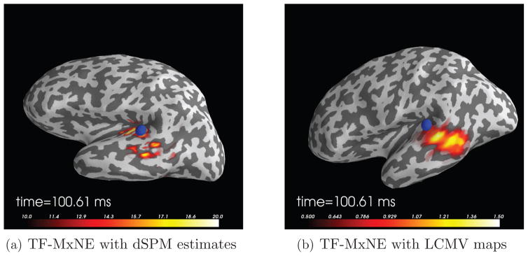
Comparison of TF-MxNE, dSPM, and LCMV for an auditory stimulation. The images show the TF-MxNE solutions overlayed with dSPM estimates (a) and LCMV output map (b) 100 ms after stimulation. Since LCMV does not exploit the cortical orientation information, the map peaks are located at the gyri, below the auditory cortex in the temporal lobe.

5.2.2. Visual data

We used the same model parameters (loose orientation, depth bias, scalar weighting, λ_time and Gabor dictionary) as for the auditory condition. The spatial regularization was however changed to λ_space = 30% of ${\lambda }_{\text{space}}^{max}$. Results are presented in Figure 8.

Figure 8.

Results obtained with TF-MxNE for a visual stimulation (checkerboard stimulus in the left visual field) with unfiltered MEG data. Estimation was performed with a loose orientation (parameter 0.2), with a depth compensation of 0.9 on a set of 7498 cortical locations (G ∈ ℝ^364×22494). Estimation with λ_space = 30% of ${\lambda }_{\text{space}}^{max}$ leads to 3 active brain locations in the contralateral visual cortex (V1 and V2). TF-MxNE leads to smooth time courses and zeros during baseline.

Figure 8(a) presents the raw evoked response, restricted to the gradiometers. Sources reconstructions lead to three dipoles. According the automatic parcellation of the cortex provided by FreeSurfer, two sources are localized in the early visual cortex V1, while a third one is positioned on the dorsal part of the secondary visual cortex (V2). One can then quantify the temporal latencies. Between the largest peaks for the early V1 sources the latency is zero which suggests that it could be the same source not properly modeled with a single cortically constraint dipole. Between the V1 sources and the later V2 source the latency is equal to 7 ms, which is very reasonable according to the literature [5]. Here again one can observe the source time series are truely set to zero during baseline.

Using the implementation details provided in Section 4.1, the computation on each dataset presented in this section takes about 30 seconds on a standard laptop computer.

For comparison with alternative solvers, we show in Figure 9 the TF-MxNE source locations superposed to dSPM reconstructions and LCMV beamformer [44] outputs at the time instants corresponding to the two peaks in the evoked response. For LCMV, the data covariance was computed from 40 ms to 150 ms. One can observe that for the early peak all three methods agree to locate the main source in V1 along the calcarine fissure, although dSPM and LCMV lead to more smeared maps. For the second peak, it is pleasing to see how well LCMV and TF-MxNE agree on the site of the blue source, located in the dorsal part of V2 according to the FreeSurfer parcellation.

Figure 9.

Comparison of TF-MxNE, dSPM, and LCMV for a visual stimulation (checkerboard stimulus in the left visual field). The images show the TF-MxNE solutions overlayed with dSPM estimates (a) and LCMV output maps (b) for two different time points corresponding to the main peaks in Figure 8(a). For the early peak, there is a very good agreement between all three methods although dSPM and LCMV maps are smeared in space. For the later peak, LCMV and TF-MxNE agree on the location of the blue source.

6. Discussion

While time-frequency analysis is commonly used in the context of M/EEG both in the sensor and source space, it has rarely been used to better model the source dynamics in the context of the inverse problem. Some earlier contributions, such as [10, 13, 26, 28], apply a two-step approach. First TF atoms are estimated from sensor data, typically with greedy approaches like Matching Pursuit. Subsequently, the inverse problem is solved on the selected components using parametric [13], scanning [26] or distributed methods [10, 28]. Such methods suffer from several limitations. They implicitly assume that the source waveforms correspond to single TF atoms, while real brain signals are better modeled by a combination of atoms as proposed in this contribution. In addition, estimation errors made in the first step have a direct impact on the accuracy of the sources estimates. This is a particularly critical issue since the first step does not take into account the biophysics of the problem, i.e., the solution of the forward problem.

Certainly motivated by the ability of dipole fitting methods to explain M/EEG data, spatial sparsity of source configurations has also been a recurrent assumption to improve the performance of the M/EEG distributed source models. However, variational formulations based on mixed-norms [34, 15], or Bayesian methods with sparsity inducing mechanisms [11, 46] that have been proposed so far in the literature do not model the transient oscillatory nature of brain signals. These approaches make the strong assumption that the source time courses are stationary. For example, results are strongly dependent on the time interval considered. Also the solutions obtained by these solvers are invariant with respect to the permutation of the columns of M, i.e., the temporal sequence of the data is immaterial. This contribution does not suffer from this limitation by explicitly modeling the temporal dynamics of the signals.

To improve over MNE type methods, by removing the assumption of a constant SNR over time and to correlate the time instants together, one should mention recently proposed state-space models based on Kalman filters and smoothers [29, 25]. Such methods, although promising, are still computationally demanding and could suffer from more practical issues like rather long time series to estimate the latent parameters reliably and the necessity to work with fixed orientations.

In [40], an inverse solver that models the transient and non-stationary responses in M/EEG is proposed. A probabilistic model with wavelet shrinkage is employed to promote spatially smooth time courses. The estimation however relies on model approximations with no guarantee on the solution obtained. The most related work to ours, beyond the field of M/EEG, is probably [31] where sparsity is also promoted on the TF decompositions. The related optimization problem, is however solved with a truncated Newton method which can only be applied to differentiable problems. The non-differentiability of the cost function is tackled by using smooth approximation in the minimization. Moreover, Newton methods are known to be fast in the neighborhood of the solution, but little is known about the global convergence rate. In [33], it is proved that a suitable Newton technique has the same rate of convergence as the accelerated first order schemes like the one we are employing in TF-MxNE. In this contribution, we do not address the problem of learning spatial basis functions as in [43] as doing so would make the cost function non-convex, which would deteriorate the speed of convergence and would also make the solver dependent on the initialization. However, using a pre-defined dictionary of spatial basis functions in line with [3, 21] and multiplying the gain matrix with this dictionary, our prior could be used to estimate spatially extended sources with temporally smooth waveforms. This would, however, be significantly more computationally expensive.

In this work, we demonstrated how physiologically motivated priors for brain activations can be accounted for in a mathematically principled framework in M/EEG source analysis. Using a composite prior, the sparsity of spatial patterns, the temporal smoothness, and the non-stationarity of the source signals were well recovered. Thanks to the structure of the cost function considered, mainly its convexity, an efficient optimization strategy was proposed. The problem being convex, the solver is not affected by improper initialization and cannot be trapped in local minima. Simulations indicated benefits of the approach over alternative solvers, while results with well understood MEG data confirm the accuracy of the reconstruction with real signals. Both results show that our solver is a promising new approach for mining M/EEG data.

Highlights.

• our method solves the M/EEG inverse problem without assuming source stationarity

• we localize sources in space, time and frequency in one step

• we provide results on simulations and two publicly available MEG datasets

• the solver uses short time Fourier transforms (STFT) and modern optimization techniques

• the solver is tractable and fast on real data

References

- 1.Balian R. Un principe d’incertitude en théorie du signal ou en mécanique quantique. Compte Rendu de l’Académie des Sciences; Paris. 1981. p. 292. Série 2. [Google Scholar]
- 2.Beck A, Teboulle M. A fast iterative shrinkage-thresholding algorithm for linear inverse problems. SIAM Journal on Imaging Sciences. 2009;2 (1):183–202. [Google Scholar]
- 3.Bolstad A, Veen BV, Nowak R. Space-time event sparse penalization for magneto-/electroencephalography. NeuroImage. 2009 Jul;46 (4):1066–81. doi: 10.1016/j.neuroimage.2009.01.056. [DOI] [PMC free article] [PubMed] [Google Scholar]
- 4.Chen S, Donoho D, Saunders M. Atomic decomposition by basis pursuit. SIAM Journal on Scientific Computing. 1998;20 (1):33–61. [Google Scholar]
- 5.Cottereau B, Lorenceau J, Gramfort A, Clerc M, Thirion B, Baillet S. Phase delays within visual cortex shape the response to steady-state visual stimulation. NeuroImage. 2011;54 (3):1919– 1929. doi: 10.1016/j.neuroimage.2010.10.004. [DOI] [PubMed] [Google Scholar]
- 6.Dale A, Liu A, Fischl B, Buckner R. Dynamic statistical parametric neurotechnique mapping: combining fMRI and MEG for high-resolution imaging of cortical activity. Neuron. 2000;26:55–67. doi: 10.1016/s0896-6273(00)81138-1. [DOI] [PubMed] [Google Scholar]
- 7.Dale A, Sereno M. Improved localization of cortical activity by combining EEG and MEG with MRI cortical surface reconstruction: a linear approach. J Cogn Neurosci. 1993;5(2):162–176. doi: 10.1162/jocn.1993.5.2.162. [DOI] [PubMed] [Google Scholar]
- 8.Daubechies I. Ten lectures on Wavelets. SIAM-CBMS Conferences Series.1992. [Google Scholar]
- 9.Donoho D. De-noising by soft-thresholding. Information Theory, IEEE Transactions on. 1995 May;41 (3):613–627. [Google Scholar]
- 10.Durka PJ, Matysiak A, Montes EM, Valdés-Sosa P, Blinowska KJ. Multichannel matching pursuit and EEG inverse solutions. Journal of Neuroscience Methods. 2005;148 (1):49– 59. doi: 10.1016/j.jneumeth.2005.04.001. [DOI] [PubMed] [Google Scholar]
- 11.Friston K, Harrison L, Daunizeau J, Kiebel S, Phillips C, Trujillo-Barreto N, Henson R, Flandin G, Mattout J. Multiple sparse priors for the M/EEG inverse problem. Neuroimage. 2008 Feb;39 (3):1104–20. doi: 10.1016/j.neuroimage.2007.09.048. [DOI] [PubMed] [Google Scholar]
- 12.Gabor D. Theory of communication. J IEEE. 1946;93:429– 457. [Google Scholar]
- 13.Geva AB. Spatio-temporal matching pursuit (SToMP) for multiple source estimation of evoked potentials. Electrical and Electronics Eng. 1996:113–116. [Google Scholar]
- 14.Gorodnitsky I, George J, Rao B. Neuromagnetic source imaging with FOCUSS: a recursive weighted minimum norm algorithm. Electroencephalography and Clinical Neurophysiology. 1995 Jan;95 (4):231–251. doi: 10.1016/0013-4694(95)00107-a. [DOI] [PubMed] [Google Scholar]
- 15.Gramfort A, Kowalski M, Hämäläinen M. Mixed-norm estimates for the M/EEG inverse problem using accelerated gradient methods. Physics in Medicine and Biology. 2012 Mar;57 (7):1937–1961. doi: 10.1088/0031-9155/57/7/1937. [DOI] [PMC free article] [PubMed] [Google Scholar]
- 16.Gramfort A, Papadopoulo T, Olivi E, Clerc M. OpenMEEG: opensource software for quasistatic bioelectromagnetics. BioMed Eng OnLine. 2010;9 (1):45. doi: 10.1186/1475-925X-9-45. [DOI] [PMC free article] [PubMed] [Google Scholar]
- 17.Gramfort A, Strohmeier D, Haueisen J, Hämäläinen M, Kowalski M. Functional brain imaging with m/eeg using structured sparsity in time-frequency dictionaries. In: Székely G, Hahn H, editors. Information Processing in Medical Imaging. Vol. 6801 of Lecture Notes in Computer Science. Springer; Berlin / Heidelberg: 2011. pp. 600–611. [DOI] [PubMed] [Google Scholar]
- 18.Grosenick L, Klingenberg B, Knutson B, Taylor JE. A family of interpretable multivariate models for regression and classification of whole-brain fMRI data. 2011. pre-print. [Google Scholar]
- 19.Hämäläinen M, Ilmoniemi R. Interpreting magnetic fields of the brain: minimum norm estimates. Med Biol Eng Comput. 1994 Jan;32 (1):35–42. doi: 10.1007/BF02512476. [DOI] [PubMed] [Google Scholar]
- 20.Haufe S, Nikulin VV, Ziehe A, Müller KR, Nolte G. Combining sparsity and rotational invariance in EEG/MEG source reconstruction. NeuroImage. 2008 Aug;42 (2):726–38. doi: 10.1016/j.neuroimage.2008.04.246. [DOI] [PubMed] [Google Scholar]
- 21.Haufe S, Tomioka R, Dickhaus T, Sannelli C, Blankertz B, Nolte G, Müller KR. Large-scale EEG/MEG source localization with spatial flexibility. NeuroImage. 2011;54 (2):851–859. doi: 10.1016/j.neuroimage.2010.09.003. [DOI] [PubMed] [Google Scholar]
- 22.Jaros U, Hilgenfeld B, Lau S, Curio G, Haueisen J. Nonlinear interactions of high-frequency oscillations in the human somatosensory system. Clin Neurophysiol. 2008;119 (11):2647–57. doi: 10.1016/j.clinph.2008.08.011. [DOI] [PubMed] [Google Scholar]
- 23.Jenatton R, Mairal J, Obozinski G, Bach F. Proximal methods for hierarchical sparse coding. The Journal of Machine Learning Research. 2011 Jul;12:2297–2334. [Google Scholar]
- 24.Kybic J, Clerc M, Abboud T, Faugeras O, Keriven R, Papadopoulo T. A common formalism for the integral formulations of the forward EEG problem. IEEE Transactions on Medical Imaging. 2005;24 (1):12–28. doi: 10.1109/tmi.2004.837363. [DOI] [PubMed] [Google Scholar]
- 25.Lamus C, Hmlinen MS, Temereanca S, Brown EN, Purdon PL. A spatio-temporal dynamic distributed solution to the meg inverse problem. NeuroImage. 2012;63 (2):894– 909. doi: 10.1016/j.neuroimage.2011.11.020. [DOI] [PMC free article] [PubMed] [Google Scholar]
- 26.Lelic D, Gratkowski M, Valeriani M, Arendt-Nielsen L, Drewes AM. Inverse modeling on decomposed electroencephalographic data: A way forward? Journal of Clinical Neurophysiology. 2009;26 (4):227–235. doi: 10.1097/WNP.0b013e3181aed1a1. [DOI] [PubMed] [Google Scholar]
- 27.Lin F, Belliveau J, Dale A, Hämäläinen M. Distributed current estimates using cortical orientation constraints. Hum Brain Mapp. 2006;27:1–13. doi: 10.1002/hbm.20155. URL http://doi.wiley.com/10.1002/hbm.20155. [DOI] [PMC free article] [PubMed] [Google Scholar]
- 28.Lina J, Chowdhury R, Lemay E, Kobayashi E, Grova C. Wavelet-based localization of oscillatory sources from magnetoencephalography data. Biomedical Engineering, IEEE Transactions on. 2012;(99):1. doi: 10.1109/TBME.2012.2189883. [DOI] [PubMed] [Google Scholar]
- 29.Long CJ, Purdon PL, Temereanca S, Desai NU, Hämäläinen MS, Brown EN. State-space solutions to the dynamic magnetoencephalography inverse problem using high performance computing. Annals of Applied Statistics. 2011;5 (2B):1207–1228. doi: 10.1214/11-AOAS483. [DOI] [PMC free article] [PubMed] [Google Scholar]
- 30.Matsuura K, Okabe Y. Selective minimum-norm solution of the biomagnetic inverse problem. IEEE Trans Biomed Eng. 1995 Jun;42 (6):608–615. doi: 10.1109/10.387200. [DOI] [PubMed] [Google Scholar]
- 31.Model D, Zibulevsky M. Signal reconstruction in sensor arrays using sparse representations. Signal Processing. 2006;86 (3):624– 638. [Google Scholar]
- 32.Mosher J, Leahy R, Lewis P. EEG and MEG: Forward solutions for inverse methods. IEEE Transactions on Biomedical Engineering. 1999;46 (3):245–259. doi: 10.1109/10.748978. [DOI] [PubMed] [Google Scholar]
- 33.Nesterov Y, Polyak B. Cubic regularization of newton’s method and its global performance. Mathematical Programming. 2006;108 (1):177–205. [Google Scholar]
- 34.Ou W, Hämaläinen M, Golland P. A distributed spatio-temporal EEG/MEG inverse solver. NeuroImage. 2009 Feb;44 (3):932–946. doi: 10.1016/j.neuroimage.2008.05.063. [DOI] [PMC free article] [PubMed] [Google Scholar]
- 35.Pascual-Marqui R. Standardized low resolution brain electromagnetic tomography (sLORETA): technical details. Methods Find Exp Clin Pharmacology. 2002;24 (D):5–12. [PubMed] [Google Scholar]
- 36.Ramirez R, Kopell B, Butson C, Hiner B, Baillet S. Spectral signal space projection algorithm for frequency domain MEG and EEG denoising, whitening, and source imaging. Neuroimage. 2011 May;56 (1):78– 92. doi: 10.1016/j.neuroimage.2011.02.002. [DOI] [PubMed] [Google Scholar]
- 37.Scherg M, Von Cramon D. Two bilateral sources of the late AEP as identified by a spatio-temporal dipole model. Electroencephalogr Clin Neurophysiol. 1985 Jan;62 (1):32–44. doi: 10.1016/0168-5597(85)90033-4. [DOI] [PubMed] [Google Scholar]
- 38.Soendergard P, Torrésani B, Balazs P. Tech rep. Technical University of Denmark; 2009. The linear time frequency toolbox. [Google Scholar]
- 39.Tibshirani R. Regression shrinkage and selection via the lasso. Journal of the Royal Statistical Society Serie B. 1996;58 (1):267–288. [Google Scholar]
- 40.Trujillo-Barreto NJ, Aubert-Vázquez E, Penny WD. Bayesian M/EEG source reconstruction with spatio-temporal priors. Neuroimage. 2008;39 (1):318–35. doi: 10.1016/j.neuroimage.2007.07.062. [DOI] [PubMed] [Google Scholar]
- 41.Uusitalo M, Ilmoniemi R. Signal-space projection method for separating meg or eeg into components. Medical and Biological Engineering and Computing. 1997;35 (2):135–140. doi: 10.1007/BF02534144. [DOI] [PubMed] [Google Scholar]
- 42.Uutela K, Hämäläinen M, Somersalo E. Visualization of magnetoencephalographic data using minimum current estimates. Neuroimage. 1999;10:173–180. doi: 10.1006/nimg.1999.0454. [DOI] [PubMed] [Google Scholar]
- 43.Valdés-Sosa PA, Vega-Hernández M, Sánchez-Bornot JM, Martínez-Montes E, Bobes MA. EEG source imaging with spatio-temporal tomographic nonnegative independent component analysis. HBM. 2009 Jun;30 (6):1898–910. doi: 10.1002/hbm.20784. [DOI] [PMC free article] [PubMed] [Google Scholar]
- 44.Veen BV, Drongelen WV, Yuchtman M, Suzuki A. Localization of brain electrical activity via linearly constrained minimum variance spatial filtering. Biomedical Engineering, IEEE Transactions on. 1997 Jan;44 (9):867–880. doi: 10.1109/10.623056. [DOI] [PubMed] [Google Scholar]
- 45.Wang JZ, Williamson SJ, Kaufman L. Magnetic source images determined by a lead-field analysis: the unique minimum-norm least-squares estimation. Biomedical Engineering, IEEE Transactions on. 1992 Jul;39 (7):665–675. doi: 10.1109/10.142641. [DOI] [PubMed] [Google Scholar]
- 46.Wipf D, Nagarajan S. A unified Bayesian framework for MEG/EEG source imaging. Neuroimage. 2009 Feb;44 (3):947–966. doi: 10.1016/j.neuroimage.2008.02.059. [DOI] [PMC free article] [PubMed] [Google Scholar]