

Abstract
The primate visual cortex consists of many areas. The posterior areas (V1, V2, V3, and middle temporal) are thought to be common to all primate species. However, the organization of cortex immediately anterior to area V2 (the “third tier” cortex) remains controversial, particularly in New World primates. The main point of contention has been whether the third tier cortex consists of a single area V3, representing lower and upper visual quadrants in dorsal and ventral cortex, respectively, or of 2 distinct areas (the dorsomedial [DM] area and a V3-like area). Resolving this controversy is crucial to understand the function and evolution of the third tier cortex. We have addressed this issue in marmosets, by performing high-precision mapping of corticocortical connections in cortex bordering dorsal V2. Multiple closely spaced neuroanatomical tracer injections were placed across the full width of dorsal V2 or adjacent anterior cortex, and the location of resulting labeled cells mapped throughout whole flattened visual cortex. The resulting topographic patterns of labeled connections allowed us to define areas and their boundaries. We found that a complete representation of the visual field borders dorsal V2 and that the third tier cortex consists of 2 distinct areas. These results unequivocally support the DM model.
Keywords: area DA, corticocortical connections, dorsomedial area, primate, ventrolateral posterior area
Introduction
The primate visual cortex consists of numerous morphologically and functionally distinct areas (Felleman and Van Essen 1991), most of which have a topographic map of the visual field. Functional studies of these areas require knowledge of their precise location and boundaries. In addition, establishing similarities in the number, size, and organization of visual areas, and their location relative to one another in different primate species is crucial to understanding the evolution of visual cortex in primates. In this context, a prevailing view has been that the posterior visual areas (i.e., areas V1, V2, V3, and middle temporal [MT]) are common to all primates and thus, likely are of more ancient phylogenetic development (Kaas 1997). However, while there is widespread agreement on the location and extent of areas V1, V2, and MT in many species (Felleman and Van Essen 1991; Kaas 1997; Van Essen 2004), the organization of the “third tier” visual cortex (Allman and Kaas 1975), that is, the cortical region situated along the anterior border of V2, has been a point of contention for over 30 years.
Figure 1 depicts the 2 main competing partitioning models of this cortical region in New World monkeys. The “V3 model” (Fig. 1a) (Lyon and Kaas 2001, 2002b) is based on data obtained in Old (Zeki 1969, 1978a; Gattass et al. 1988; Lyon and Kaas 2002a) and New World monkeys. In this model, an elongated third visual area (V3) adjoins the anterior border of V2 sharing with V2 the representation of the horizontal meridian (HM) (Fig. 1c) and mirroring the retinotopy of V2. V3 represents the entire contralateral visual hemifield, with the lower quadrant mapped dorsally (in dorsal V3 or V3d) and the upper quadrant mapped ventrally (in ventral V3 or V3v) to the V2 foveal representation. In this scheme, a dorsomedial (DM) area, representing both upper and lower visual quadrants, abuts the medial portion of V3d at its vertical meridian (VM) representation. In contrast, the “DM model” (Fig. 1b) (Rosa et al. 2005), stemming from many early anatomical and physiological studies in New World primates (Allman and Kaas 1975; Spatz et al. 1987; Weller et al. 1991; Krubitzer and Kaas 1993; Rosa and Schmid 1995), views area DM as directly abutting dorsal V2 (V2d) anteromedially, at its HM representation (Fig. 1d). Thus, in the DM model there is no V3d between V2d and DM. Furthermore, in this model, the lower quadrant representation of a second area (the ventrolateral posterior area, VLP) borders V2d anterolaterally, while its upper quadrant representation adjoins ventral V2 (V2v).
Figure 1.

Two partitioning models proposed for marmoset visual cortex. The “V3” model is depicted in (a,c), the “DM” model in (b,d). (a,b) Top: Sketch of the lateral view of the marmoset brain, showing the partitioning of visual cortex between V2 and MT according to each model. Bottom: Partitioning of visual cortex, according to each model, shown onto an outline of unfolded and flattened marmoset visual cortex. The outer thin dashed outline is the outline of the dorsolateral surface of visual cortex prior to unfolding, while the outer thin solid outline is the outline of unfolded medial and ventral cortex. Middle inset: Diagram of the central 16° of the right visual hemifield; here and elsewhere in the figure, the thick dashed lines/contours represent the HM, the thick solid lines/contours the VM, the stars the fovea, the thin dotted contours the iso-eccentricity lines (numbers indicate eccentricity), and the “+” and “−” signs indicate the upper and lower visual field, respectively, with upper field regions additionally shaded in pink. + and − are indicated only for areas for which retinotopic maps have been determined by previous electrophysiological studies (adapted from: Rosa and Schmid 1995; Rosa et al. 2005). Thinner solid lines demarcating areal borders indicate uncertainty of meridian representations. The region inside the red box is schematically diagrammed in (c,d). (a) In the V3 model, V3d, representing the lower visual quadrant, is interposed between V2d and area DM. V3v, instead, representing the upper visual quadrant, abuts V2v anteriorly. Cortex between foveal V2 and MT includes posterior and anterior subdivisions of area DL/V4 (Sereno and Allman 1990; Kaas 1997). This scheme is similar to that proposed for macaque (Gattass et al. 1988; Lyon and Kaas 2002a). A modified version of this scheme in macaque, based on described connectional and functional asymmetries between V3d and V3v, views these as 2 different areas, V3 and VP, representing contralateral lower and upper visual quadrants, respectively (Burkhalter et al. 1986). (b) In the DM model, area DM, representing both upper and lower visual quadrants, directly abuts V2d anteriorly and medially. Lateral to DM+, a second visual area, VLP, also representing the entire visual hemifield, borders V2d anterolaterally and V2v anteriorly. VLP, thus, encompasses the upper field representation of V3v and parts of the lower field representation of V3d and posterior DL of the competing model. (c,d) Schematic block diagrams of cortex inside the red box in (a) and (b), respectively, showing, in color code, the representation of polar angles in each cortical area, with orange and green indicating upper and lower visual quadrants, respectively, yellow the HM and dark red and dark green the VM. In (c), the lower quadrant representation of V3d abuts and mirrors that of V2d, with the HM represented at the V2d/V3d border and the VM at the V3d/DM border. In (d), the upper quadrant representation of DM abuts V2d, with the HM represented at the V2d/DM border and the VM at the anterior DM border. In (d), the lower quadrant representation of VLP also abuts and mirrors the lower quadrant representation of V2d. Note that in both models, there exists an upper field representation (DM+) in cortex anterior to V2d, but its posterior border represents a different meridian in the 2 different models. The location of DM+ constrains the location of V3 to be posterior to it, therefore making V2d in the Lyon and Kaas (2001) model narrower than V2d in the Rosa et al. (2005) model.
These different models have resulted from different methodological approaches to partition this cortical region. The V3 model in New World primates has emerged primarily from connectional studies demonstrating projections from dorsal and ventral V1 to cortex anterior to dorsal and ventral V2, respectively (Lyon and Kaas 2001, 2002b). However, these studies provided inconclusive evidence with respect to the existence of an area V3 (Rosa et al. 2012) due to use of only one or few tracer injections in the same area, and delineation of areal boundaries that was not based on multiple objective methods. In the broader debate among competing partitioning models of cortex, it is becoming increasingly important to use multiple objective methods to delineate areal boundaries and to quantify and visualize the uncertainties associated with identifying these boundaries (Van Essen 2004).
Evidence supporting the DM model, instead, has resulted primarily from single microelectrode mapping studies demonstrating an upper quadrant representation bordering the HM representation of V2d, without an interposed retinotopic reversal of the V2 lower visual field map (corresponding to V3d). However, in these studies, scatter in receptive field position and qualitative assessment of receptive field position could have hindered the identification of a narrow V3d.
The goal of this study was to determine which of these 2 models best reflects the organization of the third tier visual cortex in New World monkeys. Resolving this issue is important to understand the function and evolution of this cortical region in primates. We addressed this issue, using a novel approach that allowed us to overcome the limitations of previous studies. Specifically, we exploited the precise topography of feedforward and feedback connections between neuronal populations in early visual areas (Angelucci et al. 2002) to finely map anatomically the retinotopically organized third tier visual cortex. We made rows of closely spaced injections of up to 7 different neuroanatomical tracers across the full width of V2d, from its VM to its HM representation, or in cortex just anterior to V2d. Furthermore, unlike previous studies, we used multiple objective criteria to delineate areal boundaries and determine the areal location of tracer injection sites. The topographic pattern of labeled connections resulting from these rows of injections, especially when judged relative to the well-described retinotopy of areas such as V1, revealed an upper visual field representation directly abutting V2d and demonstrated that 2 distinct areas (DM and VLP/V3), each representing the entire visual hemifield, border V2. These results suggest that previous functional investigations of the third tier visual cortex carried under the assumption of a V3 model may have led to attributing the properties of 2 different areas to a single area V3. Our results prompt new questions about the contribution of the third tier cortex to the dorsal and ventral streams of visual cortical processing and the evolution of this cortical region in primates.
Materials and Methods
Animals
This study was carried out in the marmoset monkey (Callithrix jacchus), a diurnal New World primate that offers several advantages as a model for studies of vision, including a small lissencephalic brain and a well-developed fovea. For this study, we analyzed data from 27 neuronal tracer injections made in 10 marmosets (5 females and 5 males; see Table 1) obtained from an in-house colony. All experimental procedures conformed to National Institutes of Health Guidelines for Animal Experimentation.
Table 1.
Summary of injection sites
| Case no. | Sex | Tracer injected | Area injected | CO stripe injected | Layers injected | Injection eccentricity (°) | Injection diameter (mm) | Dominant V1 layer projections | Dominant visual field projections | Figures |
| Rows of injections | ||||||||||
| M295 | M | CTB-647 | V2/DM+ (HM)a | NI | 1–5/6 | −3/+3 to +6 | 0.98 | Both | UVF, LVF | 3, 4b, 5, 12, Supplementary Figures 1, 2a, and 3a |
| M295 | M | CTB-555 | DM+ | — | 1–6 | +10 to +12 | 0.58 | 4A/B | UVF | 3, 4a, 5, Supplementary Figures 2b and 3b |
| M295 | M | CTBg | DM+/DA (VM) | — | 1–6 | +12 to +14/+20 | 0.73 | 4A/B | UVF | 3, 5, 12, Supplementary Figures 2a and 3a |
| M295 | M | CTB-488 | DM+/DA (VM) | — | 1–6 | +18/+20 | 1.02 | Little 4A/B | UVF | 3, 5, 12, Supplementary Figures 2b and 3b |
| M286 | M | DY | V2d/DM+ (HM)a | NI | 2–5/6 | −4/+6 to +8 | 0.85 | Both | UVF, LVF | 6, 12, Supplementary Figure 4a |
| M286 | M | CTBg | DM+ | — | 2–5/6 | +14 to +16 | 0.75 | 4A/B | UVF | 6, Supplementary Figure 4b |
| M286 | M | CTB-488 | DM+/DA (VM) | — | 1–4 | +18/+20 | 0.62 | Little 4A/B | UVF | 6, 12, Supplementary Figure 4a |
| M298 | F | DY | V2d/DM+ (HM)a | Plat/Tk | 1–6 | −3/+4 | 0.98 | Both | LVF | 12 |
| M298 | F | CTB-488 | DA/DI (VM) | — | 1–6 | +16 | 0.51 | None | UVF | 12 |
| M298 | F | CTB-555 | DA/DI | — | 1–6 | +20 | 0.72 | None | UVF | — |
| M298 | F | FB | DA/DI | — | 1–5 | +6 to +20 | 1.74 | None | UVF | — |
| M293 | F | BDA | V2d (VM) | Tn | 1–6 | −2.5 to −3 | 0.92 | 2/3 | LVF | 7, 8a,c,d, 9, 12 |
| M293 | F | CTB-647 | V2d (VM) | Tn | 1–5/6 | −3 | 0.5 | 2/3 | LVF | 7, 8a,e, 9 |
| M293 | F | DY | V2d | Pmed | 1–6 | −3 to −3.5 | 0.81 | 2/3 | LVF | 7, 8a,d, 9 |
| M293 | F | CTB-555 | V2d | Pmed/Tk | 1–6 | −3.5 to −4 | 0.53 | 2/3 | LVF | 4c, 7, 8b,f, 9 |
| M293 | F | CTBg | V2d | Tk | 1–6 | −4 | 0.86 | 2/3 | LVF | 4d, 7, 8b,c, 9 |
| M293 | F | CTB-488 | V2d (HM)a | Pmed/Tk | 1–5/6 | −4.5 to 5 | 0.66 | 2/3 | LVF | 7, 8b,e,f, 9, 12 |
| M293 | F | FB | V2d/DM+a | NI | 1–5/6 | −5.5/+8 to +10 | 1.12 | Both | LVF | 7, 8d, 9, 12 |
| M261 | F | CTB-488 | V2d/V1d (VM) | Pmed/Tk | 1–3 (V2)/4–6 (V1) | −4 | 0.4 | 2/3 | LVF | 10–12 |
| M261 | F | FB | V2d | Pmed/Tn/Tk | 2–6 | −4 to −5 | 0.57 | 2/3 | LVF | 10–12 |
| Additional injections | ||||||||||
| M217 | M | FR | V2d (VM) | NI | 1–5/6 | −3.5 | 0.67 | 2/3 | LVF | 12 |
| M223 | M | FR | V2d (VM) | Tn/Pmed | 2–6 | −2 to −3 | 0.87 | 2/3 | LVF | 12 |
| M233 | M | CTBg | V2d/DM−/+?a | NI | 1–6 | −5.5/−5/+10 | 1.08 | Both | LVF | 12 |
| M248 | F | CTB-488 | V2d?/DM+ (HM)a | NI | 1–6 | −5/+8 | 0.9 | Both | UVF | 12 |
| M248 | F | FB | V2d/DM− (HM)a | NI | 1–3 (DM)/4–6 (V2) | −8/−8 | 0.87 | 2/3b | LVF | 12 |
| M265 | F | FB | DM− (VM) | — | 1–6 | −12 | 1.65 | 4A/B | LVF | 12 |
| M286 | M | FR | V2d/DM− (HM) | NI | 2–5/6 | −6/−6 | 0.85 | Both | LVF | 12 |
Note: P, Tk, Tn: pale, thick, thin CO stripe, respectively; NI: not identifiable; UVF, LVF: upper and lower visual field, respectively. “?”: Due to border uncertainty, the injection site could have involved the indicated area. In the eccentricity column, “/” separates eccentricities of the injection site in the different cortical areas involved by the injection
Injection sites whose location corresponds to that of putative V3d.
In this case, there was no significant V1 layer 4B label because the DM side of the injection did not reach layer 4 (i.e., V1 feedforward projections to DM would be unlabeled); however, labeling pattern of interareal feedback projections and intraareal connections within DM suggested that the injection involved DM−.
Surgery and Anatomical Tracer Injections
Animals were preanesthetized with ketamine (25 mg/kg intramuscularly), intubated with an endotracheal tube, and placed in a stereotaxic apparatus. They were artificially ventilated, and anesthesia was maintained with 0.5–2% isofluorane in a mixture of 1:1 oxygen and nitrous oxide. Throughout the experiment, end-tidal CO2, ECG, blood oxygenation, and rectal temperature were monitored continuously, and repeated subdermal injections of lactated Ringers solution were made to maintain proper hydration.
Under sterile conditions, a small craniotomy and durotomy were made over the target region of the occipital cortex identified by stereotaxic coordinates. We used our own atlas of the marmoset visual cortex constructed over several years, which is based on >60 tracer injections made in the visual cortex of >25 adult marmosets. The following retrograde and anterograde anatomical tracers were used for injections (Table 1): 3% cholera toxin subunit B conjugated to alexa-488, -555 or -647 (CTB-488, CTB-555, and CTB-647, respectively; Invitrogen) in distilled water, 0.1% gold-conjugated CTB (CTBg; List Biological Labs) in distilled water, 10% fluororuby (FR, dextran tetramethylrhodamine 3000 and 10 000 MW mixed 1:1; Invitrogen) in 0.1 M phosphate-buffered (PB) saline pH 7.3, 10% biotinylated dextran amine (BDA; Invitrogen) in PB saline pH 7.3, 2% or 5% fast blue (FB; EMS-Chemie—Deutschland—GmbH) in distilled water, and 2% diamidino yellow (DY; Sigma–Aldrich) in distilled water. The tracers FR and BDA were delivered iontophoretically, using glass micropipettes of ∼15 to 20 μm tip inner diameter, and positive current in 7 s on/off cycles of 5 μA for 10–15 min. The remainder of the tracers were pressure injected using a picospritzer and micropipettes of ∼30 to 50 μm tip inner diameter (CTBg: 30–350 nL; CTB-488: 15–40 nL; CTB-555: 45–60 nL; CTB-647: 60–80 nL; FB: 30–200 nL; DY: 150 nL). In order to involve all cortical layers, each tracer was injected first at a depth of 1.1 mm from the pial surface, and then, the injection was repeated at a depth of 0.5 mm; alternatively, a single injection of a larger volume was made at 0.8 mm depth. These parameters typically yielded tracer uptake zones of ∼0.6 to 0.9 mm diameter, with a few larger or smaller injections (Table 1). To achieve high-precision topographic mapping of corticocortical connections, closely spaced injections of up to 7 different tracers were made in a single animal; these injections were delivered in an anteroposterior row involving the full width of V2d, or cortex just anterior to V2d, at the approximate mediolateral level of the upper visual field representation of DM (or DM+).
On completion of the injections, the craniotomy was filled with sterile Gelfoam, covered with sterile parafilm, and sealed with dental acrylic and the wound was sutured closed. The animals were recovered from anesthesia, and after 6–14 days survival (case M223 survived 1.5 days), they were euthanized with and overdose of sodium pentobarbital and lightly perfused transcardially with saline containing 0.5% sodium nitrate, followed by 2% paraformaldehyde in 0.1 M PB pH 7.3 for 5–7 min.
Histology
To avoid imprecise reconstructions of the labeling pattern from transverse tissue sections, we studied labeled patterns in manually unfolded and flattened visual cortex. The flattened cortex was postfixed between glass slides for 1–2 h, cryoprotected in 30% sucrose, and frozen-sectioned tangentially at 40 μm. Alternating sections were divided into 3 series; 1 series was reacted for cytochrome oxidase (CO) (Wong-Riley 1979) to reveal area and laminar boundaries, the remaining 2 series were processed to reveal the injected neuronal tracers. Specifically, for fluorescent tracers, 1 series was mounted immediately after sectioning, cover-slipped using Gel Mount (Biomeda Corp.), and analyzed under fluorescence microscopy. The third series was immunoreacted for CTB-488, BDA, or FR. Immunohistochemistry to reveal CTB-488 or FR (in different sections) was carried out by incubating sections for 24–48 h in the specific primary antibody (1:7000 rabbit anti-alexa-488 IgG or rabbit anti-fluororuby IgG, respectively), then for 1 h in 1:200 biotinylated donkey anti-rabbit IgG, followed by standard avidin-biotin complex and 3,3′ diaminobenzidine (ABC-DAB) reactions. BDA was revealed by standard ABC-DAB reactions. CTBg was revealed using silver intensification (Llewellyn-Smith et al. 1990) on the immunoreacted sections and/or on the CO-stained sections. In the latter case, CO staining was digitized prior to reacting for CTBg.
Data Analysis
Mapping of Injection Sites and Transported Label
All tracer injections used for analysis met the following 2 criteria: 1) the injection did not encroach on the white matter and 2) the tracer was transported outside the injected cortical area.
Tracer injection sites were mapped on a full series of tissue sections, aligned using radial blood vessels, and collapsed onto a 2D plane. The composite injection site was overlaid onto images of CO staining, and its areal and layer location, and diameter (extent of longest axis—Table 1) were determined. The effective tracer uptake zone for the CTB-alexas and FR was defined as the region at the injection site where no labeled cell bodies or fibers could be discerned (Ericson and Blomqvist 1988; Llewellyn-Smith et al. 1990; Luppi et al. 1990; Brandt and Apkarian 1992; Angelucci et al. 1996). For CTBg, it was defined as the dark core seen under dark field microscopy and for FB and DY, it was the region of tissue damage caused by the injected tracer (Conde 1987) visible under fluorescence illumination. In addition, most injection sites were identifiable in CO-stained sections as spots of discolored CO staining. The radial extent of injection sites, that is, the cortical layers involved (Table 1), was determined by reference to cortical layers identified in adjacent CO-stained sections. The approximate eccentricity of the injection sites was determined by reference to published electrophysiological retinotopic maps (Rosa et al. 1997, 2005) and verified by the location of transported label relative to the retinotopic maps in V1 and V2. This is acceptable in view of previous data showing a strong degree of constancy across animals in the retinotopic maps of marmoset V1 and V2 relative to a number of landmarks (Rosa et al. 1997). Note, however, that knowledge of the exact eccentricity of the injection sites was not crucial for the interpretation of our results.
The location of retrogradely labeled cells was plotted at 10×–20× using a computerized drawing program (Neurolucida, MicroBrightField Inc.) or by camera lucida (n = 5 cases). In Supplementary Figure 1, we show, as an example, an image of retrograde label at the magnification used for these plots. Whenever present, we also mapped anterogradely labeled fibers. However, most tracers produced poor anterograde label, with the exception of BDA (1 injections) and FR (3 injections), therefore, our analysis was based primarily on retrograde label. We mapped label throughout the visual cortex either in a full series of sections (1 in 3) or in at least 50% of the sections. In case M295-CTB-488, label was mapped on less than 50% of the sections, but the latter were chosen after visual inspection of all sections and provided sufficient information for the purpose of the case. Plots of label were imported into Adobe Photoshop and overlaid onto each other and onto images of adjacent CO-stained sections, using blood vessels for alignment. Delineation of areal boundaries and all measurements were performed onto these composite images as detailed in the following sections. Throughout this manuscript, we use the terms dorsal cortex and ventral cortex to designate cortical regions located dorsally and ventrally, respectively, to the foveal representation of V1 and extrastriate cortex. Within each of these 2 subdivisions (dorsal and ventral cortex), medial and lateral are used to designate locations closer and farther, respectively, to the brain midline, while anterior and posterior indicate locations farther and closer, respectively, to the occipital pole.
Assessment of Injection Site location
Because the conclusions of this study crucially depended on accurate assessment of injection site location, the latter was determined primarily on the basis of several objective criteria. Thus, while the CO-staining pattern was assessed and used as guidance (see Delineation of Areal Boundaries), we did not rely on CO staining alone to determine areal boundaries, with the exception of the V1/V2 border, which can be reliably identified in CO-stained sections. Instead, and unlike previous studies of V3/DM, we used 2 main objective criteria to determine the area location of injection sites. The first criterion was the topographic distribution of retrograde label resulting from the injections with respect to the representations of the upper and lower visual field in V1 and extrastriate cortex and with respect to the representations of the VM and HM in V1 and V2. Transported label could be reliably assigned to upper visual field or lower visual field even without direct electrophysiological confirmation because the representations of the 2 hemifields are physically separated in marmoset extrastriate cortex, being split at the foveal representation, with the lower visual field largely represented in dorsal cortex and the upper visual field in ventral cortex (Fig. 1a,b). The foveal representation is identifiable on CO-staining as the apogee of the curvature made by the V1/V2 border on the lateral surface of the brain (star in Fig. 1). From this point, the HM crosses V2 almost in a direct posterior-to-anterior direction and then curves anteromedially to reach the posterior tip of MT, where the fovea (star) is represented. In MT, the HM splits the dark CO oval region into dorsal and ventral halves representing the contralateral lower and upper visual field, respectively (Fig. 1). The distortions caused by the relieving cuts needed to flatten V1 did not allow us to localize the HM representation in V1 with high accuracy; however, overall, we were able to assign the bulk of the transported label to either dorsal or ventral V1, representing the contralateral lower and upper visual field, respectively.
Additionally, we were able to determine the location of an injection site with respect to the VM or HM, based primarily on the location of transported retrograde label in V1 and V2 relative to the V1/V2 border, which represents the VM and can be reliably identified in CO-staining alone. We relied primarily on the topographic distribution of retrograde label in V1 (and in V2 for injections located in cortex anterior to V2) because interareal feedforward connections are known to be highly retinotopic. While feedback connections in primates are also retinotopically organized, feedforward connections are less convergent, that is, spatially more restricted than feedback connections (Angelucci et al. 2002). While the HM cannot be accurately identified in V1, we were able to determine proximity of transported label to the HM, based on the label's distance from the V1/V2 border, its approximate location in V1 relative to the foveal representation and its location at the anterior border of V2. The latter border is known to represent the HM and can be identified with sufficient accuracy for the purpose of this study (see Delineation of Areal Borders).
Our second criterion for determining the areal location of injection sites was the V1 laminar distribution of retrograde label resulting from the injections. We define V1 layers using the terminology of Brodmann (1909), according to which layers 3B, 4A, and 4B correspond to layers 3Bα, 3Bβ, and 3C, respectively, of Hassler (1996). Previous studies in marmosets, which we confirm in this study (see Results), have shown that the V1 laminar pattern of label resulting from tracer injections in V2 (Federer, Ichida, et al. 2009) differs significantly from that produced by injections in DM (Rosa et al. 2009). Specifically, V2 injections have been shown to produce retrograde label predominantly (>70% of cells) in layers 2/3 and 4A, with a varying, but overall small contribution from layer 4B (ranging from 0% for injections in the V2 CO pale-medial stripes to 24% of total labeled cells after injections in thick CO stripes) (Federer, Ichida, et al. 2009). In contrast, injections in DM have been shown to produce label almost exclusively in V1 layers 4A and 4B, while injections anterior to DM in area dorsoanterior [DA]/dorsointermediate [DI] produce no V1 label (Rosa et al. 2009). These areal differences in V1 laminar input pattern aided us in assigning areal location to injection sites (see Results). V1 layers were identified by reference to immediately adjacent CO-stained sections and verified by counterstaining with Nissl, the same sections containing label, after plotting the label. The laminar location of CTBg label was determined on tissue sections that were reacted for both CO and CTBg.
Delineation of Areal Boundaries
For the purpose of this study, it was sufficient to identify the boundaries of areas V1 and V2. However, in the figures, we also show boundaries for areas MT and MT crescent (MTc). Boundaries for other extrastriate areas were delineated only when they could be identified on the basis of the topography of transported label and for areas known to have orderly retinotopic maps.
The V1/V2 border was identified in CO staining. CO staining was used as one of several criteria to identify the anterior V2 border and the outer border of MT and MTc. To this purpose, CO-stained sections were digitized at low magnification (1.25×). A minimum of 3 images of serial CO sections were overlaid and merged in Adobe Photoshop by aligning the radial blood vessels. Areas V1, V2, and MT were initially identified on these images, based on their distinct CO-staining patterns, that is, CO blobs in the V1 upper layers or uniform dark CO staining in layer 4C of V1 (Horton and Hubel 1981; Humphrey and Hendrickson 1983), CO stripes in V2 (Tootell et al. 1983), and a CO-dark elliptical patchy region corresponding to MT (Tootell et al. 1985). However, CO staining allows precise identification of only the V1/V2 border. In a previous study, we demonstrated that in CO staining, there is a positional ambiguity for the V2 anterior border of about 450 μm (Jeffs, Ichida, et al. 2009). For this reason, in the figures, we depict a “CO-defined transition zone” at the anterior V2 border, that is, a region encompassing the most anterior and posterior boundaries drawn on the basis of CO staining alone by 3 independent individuals.
To further reduce the positional ambiguity (i.e., the width) of the CO-defined transition zones in V2 and MT as well as to delineate boundaries of other cortical areas between V2 and MT, we used several additional criteria. The most important criterion was the topographic pattern of transported label resulting from tracer injections placed at known V2 and DM+ borders, that is, at the HM and VM representations of these areas (as determined based on the criteria described above). In particular, experiments in which we made rows of tracer injections across the full width of V2d or DM+ allowed us to delineate the HM and VM representations for several extrastriate areas. To describe these areas in the figures, we have adopted the nomenclature of Rosa et al. (2005, 2009) because these authors' partitioning scheme and retinotopic mapping studies of extrastriate cortex in marmoset were the most consistent with our anatomical data. For posterior parietal cortex (areas PPd, PPv, and Opt) and additional areas in dorsal cortex (medial superior temporal [MST] and fundus of the superior temporal [FST]), we did not attempt to identify areal boundaries, as these are largely unknown, and these areas show only loose retinotopic organizations. In the figures, we loosely identify the location, but not the boundaries, of these areas based on the maps of Rosa et al. (2005, 2009). Furthermore, we have labeled subdivisions of inferotemporal (IT) cortex as a single IT area. Additional criteria used to determine areal borders were 1) measurements taken from identifiable CO features (e.g., the V1 foveal representation, the V1/V2 border, etc.) using as reference previously published retinotopic maps of marmoset extrastriate cortex (Rosa and Schmid 1995; Rosa et al. 1997, 2005; Rosa and Elston 1998; Rosa and Tweedale 2000); 2) patterns of intraareal connections (e.g., injections in DM+ labeled intraareal connections that filled the whole of DM+, revealing its characteristic shape); and 3) location of injection sites straddling areal borders (as determined on the basis of the 2 objective criteria described above). Even using all of these criteria, in many instances, uncertainty still remained about the precise location of some areal boundaries; we defined these uncertainty regions as “label-defined transition zones” between areas and marked the anterior and posterior boundaries of these zones in the figures. For the purpose of the quantitative analysis described below, measurements were made using both boundaries of each transition zone.
Measurements of the Distance of the DM+ Borders and Label Reversals from the V1/V2 Border
For the quantitative analysis illustrated in Figure 12a, we measured the distance of the DM+ anterior and posterior borders from the V1/V2 border. We chose the V1/V2 border as reference because this can be reliably identified in CO staining. The DM+ borders were identified by, and measured at, the location of tracer injections straddling these borders (see Results). To measure this distance, we traced a first reference line parallel to the V2d anterior border and a second line orthogonal to the first one passing through the center of an injection site straddling one of the DM+ borders; the distance of the DM+ border from the V1/V2 border was measured along this second reference line. Because in many cases, the DM+ borders were delineated as transition zones, each border measurement consisted of 2 distances, indicated in Figure 12a as black and gray horizontal bars encompassing the extent of the transition zone at the corresponding DM+ posterior and anterior border, respectively.
Figure 12.
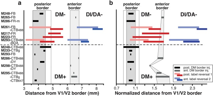
Quantitative analysis of the location of label reversals relative to the DM+ borders. (a) Distance of the DM posterior (black horizontal bars) and anterior (gray horizontal bars) borders from the V1/V2 border. Each black or gray horizontal bar represents a separate injection case (case numbers are indicated on the y-axis and apply to both a and b), and its width indicates the width of the label-defined transition zone at the area borders (see Materials and Methods). Different injections are arranged in order of mediolateral location (i.e., approximate eccentricity), with more medial locations represented at the top of the graph. Shaded gray vertical columns indicate the range of distances across the population of injection sites for the posterior (dark gray column) and anterior (light gray column) DM border, respectively. Colored horizontal bars indicate distances from the V1/V2 border of label reversal 1 (pink–red bars) and reversal 2 (blue bars) produced by rows of injections across the width of V2 (reversals 1 and 2 in Figs 8a,b and 10b) or produced by injection confined to the V1/V2 border (cases M217 FR and M223 FR in Table 1). Pink and light blue bars indicate the most posterior patch in each reversal (i.e., that resulting from the injection site at the V2d anterior border—HM representation), while red and dark blue bars indicate the most anterior patch in each reversal (i.e., that resulting from the injections site at the V1/V2 border—VM representation). Dashed horizontal line in (a) and (b) separates DM+ from DM−. (b) The distances from the V1/V2 border of DM borders and label reversals were normalized to the width of V2d at the same mediolateral level of the respective injection site or label patch. Other conventions are as in (a). Note that in (b), the anterior DM border forms a curve reminiscent of the shape of DM.
In a similar fashion, we also measured the distance from the V1/V2 border of the most posterior and anterior patches of each label reversal produced by rows of tracer injections across the width of V2d. The term label reversal is used to indicate the topographic organization of labeled connections resulting from rows of injections in V2d, which mirrored the injection site sequence. Label reversals result because the retinotopic maps in neighboring cortical areas are mirror images of each other. The distance of a label patch in each reversal was measured by first outlining the patch and then tracing 2 reference lines parallel to the V2d anterior border, one through the posterior edge of the patch outline and the other through its anterior edge; we measured the distance from the V1/V2 border of these 2 reference lines along a line orthogonal to them passing through the center of the patch.
Because the V1/V2 border is curved, often most dramatically in the same mediolateral plane as the location of DM+, the width of area V2d is not constant throughout its mediolateral extent. This generated some variability in our distance measurements. To correct for this variability, in Figure 12b, all distance measurements were normalized to the width of V2 at the corresponding mediolateral location of the injection site (or label patch). The width of V2d was measured as the distance from the V1/V2 border of the anterior and posterior boundaries of the label-defined transition zone. All measurements were corrected for 15% tissue shrinkage.
Results
Predictions of the V3 and DM Models
Figure 2 shows schematically the different results predicted by each model following rows of multiple tracer injections in cortex anterior to V2d (Fig. 2a,b) or across the full width of V2d (Fig. 2c,d), involving the representation of a full quadrant of the visual field. Figure 2a,c depicts the predictions of the V3 model and Figure 2b,d those of the DM model. These predictions are based on previous evidence that, in both cats and primates, corticocortical feedforward and feedback connections are retinotopically organized. Specifically, injections of tracers in cat area 18 (Salin et al. 1995) or macaque V2 (Angelucci et al. 2002) label coextensive fields of neurons (cells of origin of feedforward connections to V2) and axon terminals (terminations of feedback connections from V2) in striate cortex whose visual field extent is coextensive with and overlaps the aggregate receptive field size of neurons at the injected V2 site. On the other hand, feedback connections are more convergent than feedforward connections, that is, the region of visual field encoded by feedback inputs to a cortical column is larger than that encoded by feedforward inputs to the same column (Salin et al. 1992; Angelucci et al. 2002).
Figure 2.

Topography of interareal connectivity predicted by the V3 and DM models. Predictions of the V3 (a,c) and DM (b,d) models are illustrated onto outlines of unfolded and flattened marmoset visual cortex. Conventions are as in Figure 1. (a) Hypothetical row of multiple tracer injections (red arrowhead) starting in V3d near the V2d/V3d border and ending at the V3d/DM+ border. Injection sites (outlined circles) and respective resulting label (ovals) are shown in blue for injections involving the lower visual field representation of V3d and in red for the portion of the injection involving the upper visual field representation of DM. Here and in (b–d), the inset on the left indicates the eccentricities of the hypothetical tracer injection sites. The regions representing the upper visual field are shaded in pink. Only the red half of the injection involving DM+ is expected to produce significant label in upper visual field regions, nearer VM representations (red ovals). The V3d injection near the HM representation (lightest blue) is expected to produce some label in upper visual field regions confined to HM representations (open arrowheads). All other injections are expected to produce label in cortex representing the lower visual field (red asterisks). (b) A hypothetical row of injections (red arrowhead) starting in DM+, near the V2d/DM+ border and ending just anterior to the DM+ border, in the upper visual field representation of area DI/DA. Injection sites and resulting transported label are shown in blue for injections involving DM+, and in red for the injection involving DI/DA. All injections are in upper visual field cortex and therefore are expected to produce significant label in topographically corresponding cortical regions representing the upper visual field (red asterisks). The injection nearest the HM representation of the DM+ posterior border (lightest blue) may produce label in lower visual field regions but confined to HM representations (lightest blue ovals in dorsal cortex marked by open arrowheads). (c,d) Hypothetical row of tracer injections (outlined green circles marked by red arrowhead) involving the full width of V2d and expected location of resulting label (green ovals) according to each model, respectively (see Results). Numbers 1–3 indicate the label reversals resulting from the injection sequence. For simplicity, in (a–d), some areas and respective transported label are omitted.
In the V3 model, rows of tracer injections in cortex just anterior to V2d would involve area V3d (blue injections, red arrowhead in Fig. 2a). These injections are expected to produce topographically organized label in cortical regions representing the lower visual field (red asterisks) but not in cortical regions representing the upper visual field except near HM representations (open arrowheads). Label restricted to HM representations in cortex representing the upper visual field has previously been shown to result from tracer injections located near discontinuous HM representations in cortex representing the lower visual field (e.g., Felleman et al. 1997; Jeffs, Ichida, et al. 2009), such as seen in areas with a second order visual topography (e.g., V2). Thus, in the schematic example of Figure 2a, all blue injections in V3d (red arrowhead) produce label (marked by red asterisks) in dorsal V1 (V1d), V2d, dorsal MT, and dorsal MTc and in the lower visual field representation of DM (DM−), but only the lightest blue injection, which is located near the HM representation at the V2d/V3d border, produces label (lightest blue ovals marked by open arrowheads) confined to the HM representations in ventral cortical regions representing the upper visual field, such as ventral V1 (V1v), V2v, and V3v.
In the DM model, rows of tracer injections in cortex just anterior to V2d, instead, would involve area DM and depending on the mediolateral level, they may land in DM+ (blue injections marked by a red arrowhead in Fig. 2b). Injections in DM+ are expected to produce the converse topography of transported label, that is, label dominating in cortex representing the upper visual field (red asterisks) and possibly label confined to HM representations in cortex representing the lower visual field (open arrowheads). Thus, in the schematic example of Figure 2b, all blue injections in DM+ produce label (marked by red asterisks) in V1v, V2v, ventral MT, and ventral MTc and in the upper visual field representation of cortex anterior to DM+ (area DI/DA); however, only the lightest blue injection, located near the HM representation at the V2d/DM+ border, produces label (lightest blue ovals marked by open arrowheads) confined to the HM representations in dorsal cortical regions representing the lower visual field, such as V1d, V2d, DM−, and dorsal MT.
Importantly, although DM+ exists in both partitioning schemes, its posterior border represents the VM in the V3 model (Fig. 2a) but the HM in the DM model (Fig. 2b). Therefore, label produced by injections at or near the posterior border of DM+ (i.e., darkest blue injection in Fig. 2a but lightest blue injection in Fig. 2b) is expected to be at/near VM representations, if the V3 model is correct (darkest blue ovals marked by black arrows in Fig. 2a), but at/near HM representations, if the DM model is correct (lightest blue ovals marked by open arrowheads in Fig. 2b).
The presence of DM+ in both models constrains the location of putative V3d to be posterior to the DM+ posterior border. Therefore, according to the V3 model, a row of multiple tracer injections across the full width of V2d (red arrowhead in Fig. 2c), from its VM to its HM representation, should produce a row of transported label that is a mirror reversal of the injection sequence, located posterior to the DM+ posterior border (i.e., in V3d; label reversal marked as number 1 in Fig. 2c); additionally, a second row of transported label (marked as 2 in Fig. 2c), identical to the injection sequence, is expected to be located rostromedial to the posterior border of DM+ (i.e., in DM−). Instead, according to the DM model, a row of injections in V2d (red arrowhead in Fig. 2d) will produce 2 rows of transported label, both mirror reversals of the injection sequence and both located rostromedial to the posterior border of DM+, one in DM− (marked as 1 in Fig. 2d), the second in DI/DA (marked as 2 in Fig. 2d). Moreover, because of the layout of the retinotopic map in area DI/DA (Rosa and Schmid 1995) (see Fig. 1b), this second label reversal should be located well anterior to the anterior border of DM+, that is, at the parafoveal representation of DI/DA. Furthermore, because the DM model views V2d as bordered by 2 different areas, that is, DM dorsomedially and VLP dorsolaterally (Fig. 1b), it also predicts a third label reversal of the V2 injection sequence in area VLP, that is, abutting the V2d border and located laterally to the label reversal in DM (reversal marked as 3 in Fig. 2d).
Below we present results that are consistent with the scenarios depicted in Figure 2b,d, therefore supporting the DM model.
Rows of Tracer Injections in Cortex Just Anterior to V2d
To test the predictions of the 2 models illustrated in Figure 2a,b, in 3 animals, we made an anteroposterior row of several closely spaced injections of different tracers in cortex just anterior to V2d at the approximate mediolateral level of DM+ (cases M295, M286, and M298 in Table 1 and Figs 3–6).
Figure 3.

Row of 4 different tracer injections in cortex anterior to V2d. Case M295. (a) CO image resulting from the merging of 3 CO-stained sections. To avoid obscuring the CO-staining pattern, only the posterior V2 and MT borders (solid contours) and the posterior and anterior boundaries of the CO-defined transition zone (dashed contours) at the V2 anterior border are delineated. The CO-defined transition zone is indicated as a shaded gray area in (b). Colored arrows point at the location of the 4 injection sites, which are visible on the CO image as small lesions. Additional lesions are from additional tracer injections, which failed to transport. (b) The same image as in (a) is shown enlarged, with overlaid composite injection sites (encircled in black) and the mapped cell label resulting from each injection (CTB-647, blue; CTB-555, yellow; CTBg, red; and CTB-488, green). These tracers sometimes also labeled anterogradely axon fibers; their location is outlined in the figure and is shown overlaid to the retrograde label as the 2 showed the same topographic distribution. Solid and dashed white contours: areal borders representing the VM and HM, respectively. Black contours demarcate areal borders based on the topography of transported label but for which the meridian representation is unknown. Thin dashed contour outlines the dorsal surface of visual cortex prior to unfolding. “+” and “−” signs indicate cortical regions representing the upper and lower visual field, respectively. In cases in which a single border could not be unequivocally identified based on the topography of label, we delineated the outer extremes of the uncertainty border region. Black boxes in V1v and V1d indicate the location of label shown enlarged in Figure 4a,b, respectively. Scale bars here and in all remaining figures are corrected for tissue shrinkage. (c) Left: Schematic diagram of a standard unfolded and flattened visual cortex showing the location of the injection sites (outlined in black) and the outlines of the densest transported label (filled ovals) in V1 and V2 (the dense intraareal label in V2d resulted from the blue injection is omitted). Only the V1, V2, MT, and MTc borders are marked. Unfilled green oval in V1v indicates sparse label. Right: visual field map of the approximate location of the injection sites (outlined in black) and resulting V1 label (shaded colored regions). All other conventions are as in Figure 1. Same conventions are used in all remaining figures.
Figure 4.

Laminar pattern of retrograde label in V1 produced by tracer injections in different cortical areas. (a) Case M295 CTB-555. Injection in DM+. Plots of retrogradely labeled cells (yellow dots) in V1 are shown superimposed on a Nissl stain of the same section. The injection site for this case is shown in yellow in Figure 3b. Label is predominantly in layer 4B. Here and in (b–d), dotted lines indicate laminar boundaries, and numbers to the left label the respective V1 layers. (b) Case M295 CTB-647. Injection straddling the posterior DM+ border (blue injection in Fig. 3b). Plots of labeled cells (blue dots) are superimposed onto a Nissl stain of the same section. Note that to the left of the arrow label is heavy in layers 2/3, 4A, and 4B, while to the right of the arrow label is heaviest in layer 4B only. This label pattern suggests that the V1 projection to the DM side of the injection site extended farther in visual field than the projection to the V2d/V3d side of the injection; this is consistent with the larger receptive field size and magnification factor of DM (Rosa et al. 1997, 2005). Anatomical coordinates in (b) apply to (a–d). (c,d) Case M293, V2 injections. Plots of retrograde label (colored dots) in V1 from 2 adjacent tissue sections are shown superimposed to images of CO-stained sections. In (c), the black and yellow cells resulted from a CTB-555 and a DY injection, respectively, located side-by-side in the same pale-medial CO stripe of V2 (injection sites for this case are shown in black and yellow, respectively, in Figs 7b and 8a,b,d,f). Both injections produced label in layers 2/3 and 4A and virtually no label in layer 4B. The CO-stained section in (c) is immediately adjacent to the one in which the cells were plotted. In (d), the red cells resulted from an injection of CTBg located in a thick CO stripe of V2 (red injection site shown in Figs 7b and 8b,c). Cell label was plotted from the same CO section shown in (d), as this section was double stained for CO and CTBg. Label was predominant in layers 2/3, but significant label was also in layers 4A and 4B, consistent with the injection being located in a thick CO stripe of V2. The CO stripe location for these 3 V2 injection sites and quantification of resulting labeled cells in the different V1 laminae are shown in Supplementary Figure 4 and Table 4 in Federer, Ichida et al. (2009).
Figure 5.

Area V3d cannot exist between DM+ and V2d. (a) Case M295. Attempt to “fit” V3d between V2d and DM+. The hypothetical borders of putative V3d are drawn in black. Black arrows point at the site of the VM representation in V1d and dorsal MT, where transported label is expected to result from a CTB-647 injection site (blue) straddling the VM representation at the V3d/DM+ border. Clearly, there is no CTB-647 label in these regions. Here and in (c), the open arrowhead points at the CTB-647 label at the HM representation of lower field VLP. Other conventions are as in Figure 3b. (b) Same as in Figure 3c, left, but here, the borders of areas just anterior to V2d are indicated, together with schematic outlines of label within them resulting from the tracer injections. Borders and outlines of label are also shown for areas MT and MTc. (c) Same as Figure 3c, right.
Figure 6.

Row of 3 different tracer injections in cortex anterior to V2d. Case M286. (a) Image merge of 2 CO-stained sections with light delineation of the V2 and MT borders. (b) Same CO image as in (a), enlarged, with overlaid composite injection sites (DY, yellow; CTBg, red, and CTB-488, green) and the mapped cell label in V1d, V1v, and ventral extrastriate cortex resulting from them. DY label in V2d (largely intraareal label) is not mapped because the presence of 3 large injections of FB obscured it and caused tissue damage (visible as lesions in V2d). There was no V2d label resulting from the 2 other injections. Label in dorsal cortex anterior to V2d was not mapped. Arrow indicates absence of transported label at/near the VM representation in V1, where it would be expected to result from an injection site located at the VM representation at the putative V3d/DM+ border. Other conventions are as in Figure 3b. (c) Left: Schematic diagram of unfolded and flattened V1 and part of extrastriate cortex showing, for this case, the location of the injection sites (outlined in black) and the outlines of the densest transported label (filled ovals) in V1 and V2 (intra-areal label is omitted). Unfilled green oval in V1v indicates sparse label. Right: visual field map of the approximate location of the injection sites (outlined in black) and resulting V1 label (shaded colored regions). All other conventions are as in Figure 3c.
Table 1 lists all injection cases and provides for each case information on the tracer injected, the cortical area, V2 CO stripe type, and laminar location of the injected site, the injection site's diameter and approximate eccentricity, and the dominant V1 layers and visual field location of resulting retrograde label. Because this study failed to demonstrate the existence of an area V3d interposed between V2d and DM+, in Table 1, injections located posterior to DM are reported to be in V2d, with those lying in the location of putative V3d being marked by an asterisk. Inspection of Table 1 reveals that the topographic patterns of transported label and the V1 laminar distribution of retrograde label were highly consistent for injections located in the same cortical area and near the same meridian representation. All injections produced label in V1 and V2 with the exceptions of injections in area DA/DI, which consistently produced no V1 label.
Figure 3 shows a first example case (M295) in which we made a row of 4 different tracer injections (CTB-647, blue, CTB-555, yellow, CTBg, red, and CTB-488, green; Fig. 3b) aimed at involving cortex just anterior to V2d. In panel a, we show the CO-staining pattern in unfolded and flattened visual cortex, with light delineation of the CO-defined V1/V2 border, MT border, and the transition zone at the V2 anterior border. The same CO image is shown again in panel b, with overlaid injection sites and plots of their resulting label. To better reveal details of the label patterns, the same case is also shown in Supplementary Figures 2 and 3 at higher magnification and with the label resulting from different injections separated. On the left-hand side of Figure 3c, we show for the same case a schematic diagram of the injection sites and transported label in areas V1 and V2 on a standard outline of flattened marmoset visual cortex, with only the V1, V2, and MT borders indicated. On the right-hand side of Figure 3c, we show the approximate visual field location of the injection sites and of their resulting label in V1. Similar diagrams are used in all remaining figures. These diagrams are not meant to be faithful reproductions or quantifications of the actual label, but simple cartoons that highlight the location of label that is most important for the interpretation of the data in the figure.
All 4 injections in this case produced heavy label in ventral cortical regions known to represent the upper visual field, including V1v, V2v, ventral cortex anterior to V2v, ventral MT, and ventral MTc (Fig. 3b,c). Unlike the 3 most anterior injections, however, the most posterior injection (blue) also produced heavy label in dorsal cortical regions known to represent the lower visual field, such as V1d (Fig. 3b,c), V2d, dorsal MT, and dorsal MTc (Fig. 3b). This indicated that all injections involved a region of upper visual field representation, but the blue injection in addition straddled a region of lower visual field representation. Furthermore, the blue injection was located at an HM representation because label in both V1d and V1v, resulting from this injection, was located well away from the V1/V2 border (the VM representation), at/near the V1 region known to represent the HM (Fig. 3b,c). In contrast, label in V1v resulting from the red and green injections was located at the V1/V2 border, that is, near the VM representation of V1, while label from the yellow injection extended from this border well into V1v, reaching the CTB-647 (blue) label (see also Supplementary Fig. 3). This topography of label in V1 indicated that the yellow, red, and green injection sites were located progressively closer to a VM representation. Finally, the location of transported label in V1d, V1v, and V2v relative to the foveal representation in these areas indicated that the blue injection was located closer to the fovea and the other 3 injections were located at progressively more peripheral eccentricities (see Table 1). In summary, the topography of transported label, especially in V1, indicated that the blue injection was located at/near an HM representation at near-foveal eccentricities and straddled the border between a region of lower visual field representation posteriorly and a region of upper visual field representation anteriorly; the 3 more anterior injections, instead, were located in an upper visual field region at progressively more peripheral eccentricities and progressively closer to a VM representation. The blue injection must have straddled the border between DM+ and the lower visual field representation of an area posterior to DM+ (V2d or V3d). This is because, according to both partitioning models, this is the only border in this cortical region that separates an area of lower visual field representation, posteriorly, from an area of upper visual field representation anteriorly (see Fig. 1a,b). If the blue injection straddled the posterior DM+ border, then, the other injections must have been located in DM+, the most anterior possibly involving the upper visual field representation of an area anterior to DM+ (i.e., DI/DA).
We examined the V1 laminar pattern of retrograde label resulting from these 4 injections as further confirmation of their areal location (Table 1). The yellow and red injections produced the same V1 laminar pattern, suggesting they were located in the same area. This consisted of dense label primarily in layers 4A and 4B (Fig. 4a), a pattern previously described after tracer injections in area DM (Rosa et al. 2009). The blue injection produced dense label in V1 layers 2/3 and 4A and 4B (Fig. 4b). This V1 laminar pattern differs from that previously described after injections confined to V2, which instead label predominantly V1 layers 2/3 and 4A (see Materials and Methods and Fig. 4c,d). Rather, this “mixed” V1 laminar pattern produced by the blue injection suggested this lay at the border between DM and V2d or in an area that receives similar V1 laminar inputs as V2 (the V1 laminar inputs to presumptive area V3 in marmosets have not been previously described). The green injection, instead, produced very sparse label in V1 (for a magnified view of this label, see Supplementary Fig. 3b), which was confined to layers 4A and 4B, suggesting it straddled the border between areas DM+ and the upper visual field representation of area DI/DA. This interpretation is consistent with previous reports that DI/DA, an area located just anterior to DM, does not receive V1 inputs and that its posterior border shared with DM represents the VM (Rosa et al. 2009). In conclusion, the topography and V1 laminar pattern of label resulting from these 4 injections indicated that they involved the full width of the upper visual field representation of area DM, with the most posterior (blue) and anterior (green) injections encroaching into adjacent areas. Further evidence that these injections involved DM+ was the observation that the CTB-555 (yellow) injection, which lay in the middle of DM+, produced a dense local label that filled almost the entire area, revealing a shape that is consistent with that of DM+ previously described by Rosa et al. (2005, 2009) (Fig. 5a and Supplementary Fig. 2b).
Which border did the CTB-647 (blue) injection site straddle? The V2d/DM+ border or the V3d/DM+ border? In Figure 5a, we attempt to fit an area V3d between V2d and DM+. The anterior border of this putative V3d is constrained by the location of the blue injection, as we have established above that the latter encroached into DM+. We depict 2 possible locations for the posterior borders of putative V3d, assuming a 1- or 2-mm-wide V3d, respectively, according to previous reports (Lyon and Kaas 2001). According to the V3 model, the anterior border of V3d represents the VM (Fig. 1a,c), therefore, an injection straddling, this border is expected to produce label at VM representations (darkest blue ovals marked by a black arrow in Fig. 2a). However, the blue injection produced no label at or near the VM in V1 or dorsal MT (arrows in Fig. 5a), but it produced label at/near the HM representation of V1. These results demonstrate that the posterior DM+ border represents the HM and thus suggest that this border separates V2d from DM+. Note that, although in ventral cortex representing the upper visual field, label resulting from the CTB-647 (blue) injection extended nearly the full width of the areas (V2v, ventral lateral anterior [VLA,] ventral MT, and ventral MTc), from their HM to near their VM representations (Fig. 3b,c), this is not suggestive of the injection site involving a VM representation at the anterior V3d border. Because V3d represents the lower visual field, there should be no label in upper field cortex resulting from an injection in V3d except possibly at HM representations (open arrowheads in Fig. 2a). Rather, the wide CTB-647 (blue) label in ventral cortex suggests significant DM+ involvement because at near-foveal eccentricities in DM+, the HM and VM are very close to each other. Therefore, the results from case M295 are consistent with the DM model predictions illustrated in Figure 2b but not with the V3 model predictions illustrated in Figure 2a.
An alternative interpretation of these results is that a V3d exists between V2d and DM+, but its anterior border shared with DM+ represents the HM (Fig. 5a). Since the anterior V2 border is also known to represent the HM, then if a V3d exists between V2d and DM+, both its anterior and posterior borders must represent the HM, leaving unclear where the VM would be represented in V3d. A more likely explanation for this case is that the blue injection straddled the border between V2d and DM+ and that a V3d does not exist between these 2 areas. Figure 5b,c summarizes our interpretation of this case. The figure shows the same schematic diagram of Figure 3c, but we have added borders of areas lining V2 anteriorly, and the label within these areas resulted from the tracer injections (intraareal label is omitted). Label in MT and MTc is also shown. Note that, as predicted by the DM model (Fig. 2b, open arrow in dorsal VLP), the CTB-647 (blue) injection also produced label at the HM representation of a second area bordering V2d anteriorly and DM+ laterally, that is, in the lower visual field representation of area VLP (Fig. 5a,b, open arrowhead).
One last point that deserves discussion is that all 4 injections in case M295 produced a narrow strip of patchy label lining the HM representation at the posterior and medial borders of lower field DM, approximately between 6° and 16° eccentricity (Fig. 3b and Supplementary Fig. 2). We interpret this label as reflecting connections made across the discontinuous HM representations bordering DM+ posteriorly and medially and area DI/DA medially. In general, we found these projections following tracer injections almost anywhere within these 2 areas, likely due to these areas' small size and large receptive fields (which likely cross the HM of the visual field). We think it is unlikely that label in this region represents interareal projections from DM+ to presumptive V3d since similar projections would also be expected to occur at the HM representation of DM−, yet, there is no other such label in cortex dorsal to DM+.
Figure 6 illustrates a second example case (M286) in which we made a row of 3 different tracer injections (DY, yellow, CTBg, red, and CTB-488, green) aimed at involving V2d and cortex just anterior to it, at the approximate mediolateral level of DM+. For this case, we only mapped label in V1d, V1v, V2v, and ventral cortex anterior to V2v, as the topography of transported label in these areas was sufficient for the interpretation of the case. DY, but not CTBg or CTB-488, produced cell label in V2d, but this was not mapped because it was obscured by 3 large injections of FB in this area (not used for the purpose of this study) and the tissue damage caused by them (visible in Fig. 6a,b as lesions). Label in ventral cortex for this case is shown enlarged in Supplementary Figure 4. This case closely resembled case M295 discussed above. Specifically, all injections produced dense label in upper field V1 and V2 (i.e., in V1v and V2v; Fig. 6b,c) indicating they involved cortex representing the upper visual field. The most posterior (yellow) injection in addition produced label in the lower visual field region of V1, that is, in V1d, indicating it straddled the border between a lower visual field region and an upper visual field region. While label from the yellow injection was located at/near the HM representation of V1v, V1d, and V2v, label from the 2 anterior injections was located at or near the VM representation of V1v and V2v. In addition, label in V1v and V2v arising from these 3 injections showed a progression from parafoveal eccentricities, for the most posterior (yellow) injection, toward more peripheral eccentricities, for the 2 anterior injections. The V1 laminar pattern of label resulting from the green injection consisted of sparse label in layers 4A and 4B; the red injection produced a pattern typically observed after injections in DM (layers 4A and 4B) and the yellow injection produced a mixed laminar pattern (both layers 2/3 and 4A and 4B heavily labeled). In summary, the topography and the V1 laminar pattern of transported label resulting from these injections indicated that the posterior injection straddled the posterior DM+ border, the red injection was located in DM+ near its anterior border and the green injection straddled the anterior DM+ border. The narrower width of the DY (yellow) label in V2v (Fig. 6b) compared with the CTB-647 (blue) label in case M295, which instead extended much of the anteroposterior width of V2v (Fig. 3b), suggested the DY injection site was located more peripherally in DM+ (where the HM and VM representations are not as close to each other as near the foveal representation). Like the blue injection in case M295, label from the yellow injection site in both dorsal (V1d) and ventral (V1v and V2v) cortex was located primarily at HM representations. This suggests that DM+ shares an HM representation at its posterior border either with V2d or with a V3d whose anterior and posterior borders both represent the HM (i.e., the same rationale as in Fig. 5a also applies to case M286 DY). Figure 6c summarizes our interpretation of this case, that is, the yellow injection straddled the border between V2d and DM+ because an area V3d cannot exist between them, while the red and green injections were located at/near the anterior border of DM+.
A third example case (M298, data not shown; Table 1) received a row of 4 tracer injections in cortex just anterior to V2d. The most posterior injection straddled the border between a region of upper visual field, anteriorly (DM+), and a region of lower visual field, posteriorly, indicating it was located at the posterior DM+ border. Instead, the 3 anterior injections were located in a region of upper visual field and received no inputs from V1, indicating the injections were located in area DI/DA. Label resulting from the posterior injection, as in cases M295 and M286 discussed above, was also located at the HM representations of V1d, V1v, and V2v, again indicating that the injection straddled the border between V2d and DM+.
Rows of Tracer Injections across the Full Width of V2d
To test the models' predictions illustrated in Figure 2c,d, in 2 animals, we made rows of several different tracer injections across the full width of V2d (cases M293 and M261, Table 1 and Figs 7–11).
Figure 7.

Row of 7 different tracer injections across the width of V2d: low magnification. Case M293. (a) Image merge of 3 CO-stained sections with light delineation of the V2 and MT borders. Arrows point at the location of the DY (yellow), CTB-555 (black), CTB-488 (green), and FB (blue) injection sites, visible as small lesions or discolorations of CO staining. (b) Same image as in (a), enlarged, with overlaid composite injection sites and mapped cell label (BDA, orange; CTB-647, pink; DY, yellow; CTB-555, black; CTBg, red; CTB-488, green; and FB, blue). The BDA injection site produced almost exclusively anterograde label; labeled fibers were drawn in extrastriate cortex but not fully in V1, where the location of BDA label is instead indicated as a shaded orange area. (c) Left: Diagram of injection sites in V2d and transported label in V1d, V1v, V2v, and dorsal cortex anterior to V2d illustrating the 3 label reversals (numbered 1–3) observed for this case. For clarity of illustration, only the orange, pink, black, and green injections and their resulting label are shown. Note that orange and pink labels largely overlap, except in reversal 2, which showed no transport from the pink injection. Right: Approximate visual field location of the pink, black, and green injections and their respective V1 label; the visual field map of the BDA (orange) label in V1 largely overlaps that of the pink label and thus is not shown. Other conventions are as in Figure 3.
Figure 8.

Row of injections across the width of V2d: high magnification. Case M293. (a,b) Enlarged images of injection sites and resulting label in dorsal cortex from Figure 7. In (a), only label resulting from the 3 posterior injections is shown, while in (b), only label resulting from the 3 anterior injections is shown. The FB (blue) injection is not shown in (b) because it straddled the anterior border of V2d, thus involving 2 areas. Black and blue outlines in (a) and (b), respectively, outline the CTB-555 and FB injection sites, respectively. Numbers 1–3 indicate the 3 label reversals. (c–f) Portions of the images in (a,b) are further enlarged to better illustrate the 3 label reversals in cortex anterior to V2d. Only 2 or 3 injection sites and their resulting label are shown in each panel for clarity of illustration.
Figure 9.
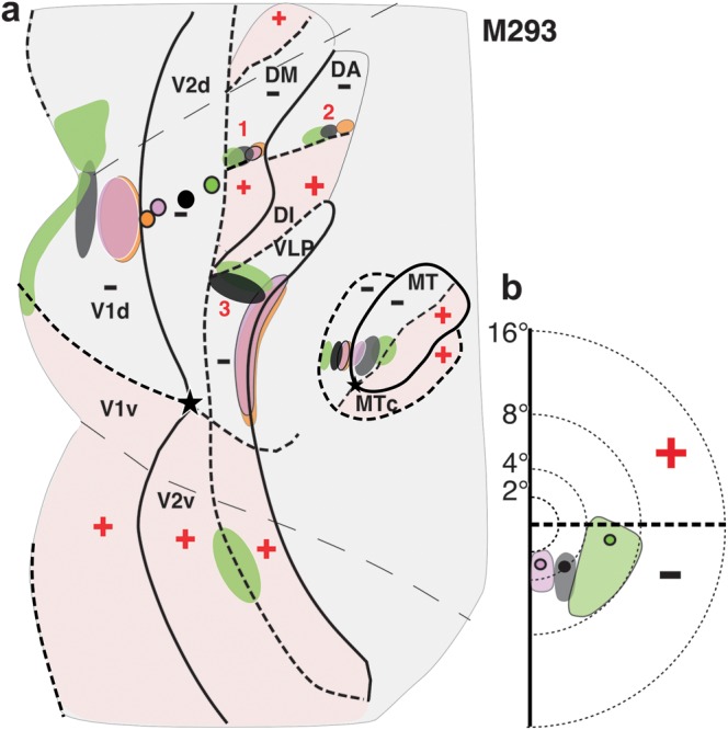
Summary of areal location of tracer injections and transported label for case M293. (a) Same as in Figure 7c, left, but here, the borders of areas just anterior to V2d are indicated, together with outlines of label within them resulting from the tracer injections. Borders and outlines of label are also shown for areas DI/DA, MT, and MTc. (b) Same as Figure 7c, right.
Figure 10.

Row of tracer injections across the width of V2d. Case M261. (a) Image merge of 3 CO-stained sections with light delineation of the V2 and MT borders. The pale CO spot (blue arrow) is the location of the FB injection site; the green arrow points at the location of the CTB-488 injection site. (b) The same image as in (a), enlarged, with overlaid composite injection sites and the mapped cell label (CTB-488, green and FB, blue). Three different tracer injection sites were made in this case, but only label resulting from the most posterior and anterior injections is shown in the figure. (c) Left: Diagram of injection sites in V2d, and transported label in V1d and dorsal cortex anterior to V2d illustrating the 3 label reversals (numbered 1–3 here and in panel b) observed for this case. Right: Approximate visual field location of the tracer injections and their respective V1 label. Other conventions are as in Figure 3.
Figure 11.
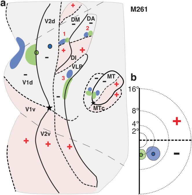
Summary of areal location of tracer injections and transported label for case M261. (a) Same as in Figure 10c, left, but here, the borders of areas just anterior to V2d are indicated, together with outlines of label within them resulting from the tracer injections. Borders and outlines of label are also shown for areas DI/DA, MT, and MTc. (b) Same as Figure 10c, right.
In case M293, 7 different tracers were injected, beginning posteriorly with an injection of BDA (orange; Figs 7 and 8a,c,f) just anterior to the V1/V2 border (VM representation) and ending anteriorly with an FB injection (blue; Figs 7 and 8d) straddling the HM representation at the anterior V2d border.
That these 7 injections were largely confined to V2d, spanning its full width was indicated by the topography of resulting retrograde (i.e., feedforward) label in V1d, which showed an orderly progression away from the VM representation at the V1/V2 border (beginning with the BDA, orange, label) toward the HM representation (ending with the FB, blue, label) (Fig. 7b). There was no switch back of the label in V1d toward the VM, indicating that none of the injections involved significantly a V3d-like area anterior to V2d. The 7 injections involved a single CO stripe cycle, several of them landing cleanly in a single stripe type (indicated in Table 1). The V1 laminar pattern of label (Fig. 4c,d and Table 1) resulting from all injections, except FB, was also consistent with that previously described in marmosets after V2 injections (Federer, Ichida, et al. 2009; see Materials and Methods). Thus, we conclude that the 6 posterior injections were located cleanly in V2d. Accordingly, label resulting from these injections was located almost exclusively in cortex representing the lower visual field (e.g., V1d, dorsal MT, and MTc; Fig. 7b,c), but the red and green injections (those closer to the HM representation of V2d) in addition produced sparse label confined to HM representations of upper visual field cortex, such as at the anterior border of V2v and possibly in V1v and ventral MT (Fig. 7b,c). The most anterior FB (blue) injection also produced label predominantly in lower visual field cortex, with sparse label lining the HM representations of upper visual field cortex. However, unlike the other injections, the blue injection produced a mixed laminar pattern of V1 label (both layers 2/3 and 4A and 4B heavily labeled; Table 1), suggesting it may have slightly encroached into cortex anterior to V2d.
The 6 injections confined to V2d produced 3 rows of primarily retrograde label, except for BDA that instead produced almost exclusive anterograde label in extrastriate areas (for BDA thus we mapped the distribution of anterogradely labeled fibers). These rows of label were all mirror reversals of the injection site sequence (label reversals are indicated as numbers 1–3 in Figs 7c and 8a,b). Reversals 1 and 2 were located anteromedial to the blue (FB) injection site (which marks the anterior V2d border). Reversal 1 was 2.1 mm wide and directly abutted the V2d anterior border; the label sequence started posteriorly with a patch of CTB-488 label (green; Fig. 8b,e,f; the FB halo made it impossible to distinguish any specific FB transport in its vicinity) largely overlapping a patch of CTBg label (red; Fig. 8b,c) and was followed in a posterior-to-anterior sequence by patches of CTB-555- (black), CTB-647- (pink), and BDA-labeled fibers (orange) (Fig. 8a–c,e,f). This label sequence lacked any DY label (yellow; Fig. 8d) likely because the DY injection was located in a pale CO stripe, a stripe type previously found not to project to area DM (Krubitzer and Kaas 1993; Federer, Jeffs, et al. 2009). Reversal 2 started 1.5 mm anterior to reversal 1 with overlapping patches of FB (blue; Fig. 8d) and CTB-488 (green; Fig. 8b,e,f), followed anteriorly by patches of CTB-555 (black; Fig. 8b,f) and BDA (orange; Fig. 8a,c,f). This label reversal lacked any label from the yellow, pink, and red injection sites, suggesting that the CO stripes involved by those injections (see Table 1) may not be connected with this cortical region. The 6 injection sites also produced a third label reversal (reversal 3 in Figs 7c and 8a,b) abutting the V2d anterior border but located lateral to the FB injection and to label reversal 1. Label reversal 3 ended anteriorly with overlapping BDA (orange), CTB-647 (pink), and DY (yellow) labels forming a vertical band running parallel to the V2d central 2° of visual field representation and then curving anteriorly for about one additional millimeter (Figs 7c and 8a). More posteriorly, CTB-555 (black), CTBg (red), CTB-488 (green), and FB (blue) each formed largely overlapping patches of label that extended from the curvature formed by the vertical band of the orange, pink, and yellow labels, all the way posteriorly to the anterior V2d border (Fig. 8b–f). Thus, there was a clear progression of label from the anterior to the posterior VLP border, despite significant overlap of label resulting from nearby injections. The latter can be explained by the large receptive field size and narrow width of VLP in this near-foveal region (Rosa and Tweedale 2000).
The pattern of these 3 label reversals in case M293 is consistent with the predictions of the DM model (Fig. 2d). Specifically, the presence of 2 reversals directly abutting V2d anteriorly (reversals 1 and 3 in Fig. 7c) is consistent with the notion of 2 areas abutting V2d, that is, DM anteromedially and VLP anterolaterally. The 2 reversals were, thus, likely located in the lower visual field regions of DM and VLP, respectively (Fig. 9). Accordingly, the vertical band of label formed by the 3 posterior injections lined the central 2–5° of the VM representation at the anterior border of VLP, following the curvature formed by the anterior arm of this cortical area, as previously described by Rosa and Tweedale (2000). These authors also described an expanded representation of the HM in this region of VLP, which is consistent with the extensive label produced by the more anterior injections, which extended much of the width of VLP (Fig. 9a).
Instead, the location and topography of reversal 2 are consistent with the interpretation that it was located in the parafoveal representation of area DI/DA, according to the retinotopic map of this area previously published by Rosa and Schmid (1995) (Fig. 1b).
We found no evidence for a label reversal mirroring the injection sequence in cortex posterior to the FB injection site (Fig. 8a), that is, in the presumptive location of V3d. The topography of reversal 2 and the presence of a third reversal abutting V2d are both inconsistent with the V3d model (Fig. 2c). In particular, reversal 3 was located more medially than the location of foveal DLc, consistent with the interpretations that it either resided in area VLP or in an area DL, which abuts V2d further medially than proposed in the scheme of Lyon and Kaas (see Fig. 1a).
A second case, M261, produced similar results to case M293 (Table 1 and Figs 10 and 11). In this case, a row of 3 different tracer injections was made (only 2 of the injections are shown in Fig. 10). The most posterior injection (CTB-488, green) straddled the V1/V2 border, while the most anterior injection (FB, blue) was located about 1–1.2 mm posterior to the V2d anterior border, as also suggested by the lack of FB label at HM representations in upper visual field cortex (Jeffs, Ichida, et al. 2009). That both injections were confined to V2d was also indicated by the V1 laminar pattern of labeled cells produced by these injections (Table 1), which was typical of V2 injections.
Like case M293, this row of injections produced 3 label reversals, that is, one in DM− (reversal 1 in Fig. 10b,c), one in DI/DA (reversal 2 in Fig. 10b,c), and the third one in VLP (reversal 3 in Fig. 10b,c). Note that in this case, reversal 3 did not directly abut V2d anteriorly, that is, at its HM representation because the most anterior V2 injection was located far from an HM representation at retinal eccentricities (approximately −5 to −6°) that are represented on the anterior arm of VLP (the VLP region directly abutting V2d anteriorly represents the central 0–3°; Fig. 1b) (Rosa and Tweedale 2000).
Location of Label Reversals Relative to the Borders of DM: Quantitative Analysis
Our results from rows of injections in V2d are qualitatively consistent with the DM model. However, to provide a quantitative validation of this model, we performed the following population analysis. We measured across all cases the distance of the DM+ borders from the well-definable V1/V2 border. We then compared this distance with that of the label reversals produced by rows of injections in V2d. The expectation is that if there exists a label reversal in dorsal V3, this should be located closer to the V1/V2 border than the DM+ posterior border. This analysis showed that label reversals 1 and 2 (Figs 8a,b, 9, 10a, and 11a) were instead both located anteriorly to the posterior border of DM+, a result that is inconsistent with the predictions of the V3 model.
To objectively identify the anterior and posterior borders of DM+, we selected among our population of injections those that straddled these borders (as determined on the basis of the 2 objective criteria described in Materials and Methods). We measured the distance of the DM+ borders from the V1/V2 border, at the mediolateral level of these injection sites (see Materials and Methods; n = 8 injections for the posterior border and 5 injections for the anterior border). In Figure 12a,b, the locations of the injections defining the posterior border of DM+ are indicated as black horizontal bars, and those defining the anterior DM+ border as gray horizontal bars. The gray shaded columns indicate the range of distances found across the population for each DM border. We then measured the distance from the V1/V2 border of the most posterior and anterior patches in label reversals 1 and 2 (Figs 8a,b, 9a, 10b, and 11a) produced by rows of injections in V2d (n = 2 cases). For this analysis, we also used 2 additional cases (M217 FR and M223 FR, Table 1) in which a single tracer injection site was placed at the V1/V2 border. The latter each produced 2 patches of label corresponding to the location of the VM representation of 2 extrastriate areas anterior to V2d (DM− and DI/DA). We measured the distance of these 2 label patches from the V1/V2 border. In Figure 12a,b, the label reversals are indicated as colored horizontal bars, with pink–red indicating reversal 1 of Figures 8a,b, 9a, 10b, and 11a and blue indicating reversal 2; in addition, dark blue and red indicate the most anterior patch in the reversal (i.e., that labeled by the injection at the VM representation of V2d) and light blue and pink indicate the most posterior patch (that resulting from the injection at the HM representation of V2d).
The population data demonstrate that the posterior border of DM+ (darker gray column in Fig. 12a) was located 3.6–4.5 mm anterior to the V1/V2 border (up to 4.9 mm, including one outlier case, M248 CTB-488). Instead, the anterior border of DM+ (lighter gray column) lay 6.2–6.8 mm anterior to the V1/V2 border. Because the anterior border of putative V3d coincides with the posterior border of DM, if a V3d exists between V2d and DM, then reversal 1 (pink–red bars) should be located posterior to this border (i.e., in V3d); reversal 2 instead should occur anterior to this border, that is, within DM−. In contrast, the most anterior patches of reversal 1 (red bars) were located 5.1–5.7 mm from the V1/V2 border, that is, anterior to the location of the posterior DM+ border (Fig. 12a). The most anterior patches of reversal 2 (dark blue bars), instead, were located 7.5–8.4 mm from the V1/V2 border, that is, anterior to the location of the anterior DM+ border.
We used the V1/V2 border for these measurements because it can be reliably identified in CO staining. However, the curvature of the V1/V2 border generates some variability in these measurements because the width of V2 varies mediolaterally. Thus, to better convey our results, we normalized all distances from the V1/V2 border to the width of V2d at the corresponding mediolateral level (for how the width of V2 was determined, see Materials and Methods). Figure 12b shows the results of this analysis after normalization. All label reversals in Figure 12b were located anterior to the DM+ posterior border and thus anterior to the putative location of V3d. Reversal 1 was in DM− and reversal 2 in DI/DA. Again, these results strongly support the DM model but not the V3 model.
Discussion
Using high-resolution mapping of topographic patterns of corticocortical connections in marmoset visual cortex and a hypothesis-testing approach, we have demonstrated that an upper visual quadrant representation directly borders dorsal V2 and that 2 areas, rather than a single area V3d, abut the anterior V2d border. A key finding was that 2 mirror reversals of the V2 lower visual field map exist in cortex just anterior to V2d, one located anteromedially (in lower visual field DM) and the other anterolaterally (in lower visual field VLP). Area VLP encompasses the territory that in macaque is usually termed the ventral posterior (VP) area (Burkhalter et al. 1986) but extends more dorsally than VP, where a representation of the lower quadrant is found (Rosa and Manger 2005). We observed no retinotopic reversal of the V2 lower visual field map between V2d and DM+, a result that is inconsistent with the central prediction of the V3 model. A second key result was that injections straddling the DM+ posterior border produced label at HM representations in striate and extrastriate cortex. This indicates that this border represents the HM and thus likely separates V2d from DM, a result that is consistent with the DM model. Inconsistent with this result, in the V3 model, the posterior DM+ border represents the VM and separates V3d from DM.
DM Borders V2d Anteriorly Not V3d
Our results are consistent with, and strengthen, previous results from electrophysiological retinotopic mapping of New World primate extrastriate cortex. These studies also showed no retinotopic reversal of the V2 lower visual field map interposed between V2d and DM+ that could indicate the existence of a V3d-like area (Allman and Kaas 1975; Krubitzer and Kaas 1993; Sereno et al. 1994; Rosa and Schmid 1995; Rosa et al. 2005). However, it was argued that a narrow V3 could have been missed in these previous studies due to the limitations of single unit electrophysiological mapping, including qualitative mapping methods, insufficiently close spacing between electrode penetrations, receptive field scatter, similarities of receptive field properties in neighboring cortical territories, and inaccuracies in recovering exact receptive field locations from electrolytic lesions.
To overcome the technical limitations of previous electrophysiological studies, we have taken advantage of the precise topographic organization of interareal connections between early visual areas to map the representation of the visual field in the third tier visual cortex. It is known that both feedforward and feedback connections in cat and primates are retinotopically organized, albeit the region of visual field encoded by feedback inputs to a cortical column is larger than that encoded by feedforward inputs to the same column (Salin et al. 1992; Angelucci et al. 2002). We used closely spaced distinguishable injections of up to 7 different anatomical tracers across the full width of V2d or adjacent anterior cortex. The resulting topographic patterns of corticocortical connections, especially of the highly retinotopic feedforward connections from V1, allowed us to determine the exact location of the DM+ posterior border and the location of the retinotopic reversals of the V2 lower visual field map relative to this border. The advantage of our approach over single unit electrophysiological mapping is that it allows us to determine the retinotopic location and connectivity of populations of neighboring cells, thus overcoming issues of sampling and receptive field scatter associated with mapping the receptive field of individual cells. In addition, our approach, which included flattening of the cortex, allowed us to overcome the issue of inaccuracies associated with reconstructions from nontangentially sectioned cortex.
Our results are inconsistent with the V3 model. Evidence supporting this model stemmed primarily from studies demonstrating that tracer injections in the upper visual field and lower visual field representations of V1 produced label in cortex just anterior to V2d and V2v, respectively (Lyon and Kaas 2001, 2002b). Although these studies indeed provided new evidence that cortex adjoining V2v anteriorly is connected with area V1, much like cortex adjoining V2d anteriorly, this evidence was inconclusive with respect to demonstrating the existence of an area V3. In particular, these same results are also consistent with the existence of 2 different areas bordering V2d and V2v, for example, DM and VLP, both connected with V1 (Rosa et al. 2012). These results were ambiguous because those studies used only single or few tracer injections within an area, did not use multiple objective methods to delineate areal boundaries and often disregarded the well-documented retinotopic organization of interareal connections. We contend that CO or myelin staining alone is insufficient to delineate areal boundaries with accuracy (Jeffs, Ichida, et al. 2009) and that the topographic distribution of retinotopically organized interareal connections is a more powerful tool to visualize areas and their boundaries (especially when used in conjunction with histochemical methods).
To overcome the limitations of these previous anatomical studies and of other studies based primarily on single tracer injections (Krubitzer and Kaas 1993; Beck and Kaas 1998; Rosa et al. 2005), our approach of using rows of multiple closely spaced tracer injections involving known meridian representations of V2d or DM, allowed us to identify areal boundaries and areal location of injection sites based on the topographic pattern of the resulting labeled connections. Furthermore, we used the laminar pattern of retrograde label in V1 produced by each injection as an additional objective criterion to assign injection sites to specific cortical areas.
Functional Implications of the DM Model: 2 Different Areas rather than a Single Area
Consistent with the DM model, our results suggest that area DM abuts V2d medially and a second area abuts V2d laterally. This was suggested primarily by the observation of 2 label reversals abutting V2d, one located medial to DM+ and the other lateral to it. The width of these label reversals and the specific pattern of label we observed in these areas are consistent with the shape and retinotopic organization of the lower visual field representations of areas DM of Rosa et al. (2005, 2009) and area VLP of Rosa and Tweedale (2000).
In contrast to our findings, the V3 model views a single area V3 lining much of V2, except at its foveal representation, where the foveal representation of area DLc/V4 may directly border V2 anteriorly (Fig. 1a) (but see Schira et al. 2009). According to this model, thus, rows of injections across the width of V2d at parafoveal eccentricities are not expected to produce 2 label reversals abutting V2d but rather a single reversal in V3d. We could not confirm this prediction.
An important functional implication of having a DM, rather than a V3, model of visual cortex organization is that the third tier visual cortex does not consist of a single area V3 lining much of V2 but rather it contains 2 different areas, DM and VLP, likely having different connectivity and function. Previous anatomical studies have shown that DM is more heavily connected with the dorsal stream (Jeffs, Federer, et al. 2009; Rosa et al. 2009), a finding that is also supported by recent functional studies of this area in marmosets (Lui et al. 2006). Specifically, the preference of DM cells' receptive fields for large moving patterns (virtually no surround inhibition) and low spatial frequencies and this area's emphasis on peripheral vision have led Lui et al. (2006) to suggest that DM plays a role in the analysis of optic flow patterns experienced during locomotion. In contrast, while connectional data are not available for VLP, previous functional studies of this area have indicated that VLP emphasizes central vision, and its cells' receptive fields are small orientation selective and direction insensitive (Rosa and Tweedale 2000). This suggests that VLP belongs to the ventral stream of visual processing. Based on these response properties, it has been suggested that DM and VLP are the homologues of human areas V6 (Pitzalis et al. 2010) and V3 (Rosa and Manger 2005), respectively.
Clearly, investigations of the function of the third tier visual cortex carried under the assumption of a V3 model of extrastriate cortex organization, would lead to attribute the response properties and connectivity of 2 very different areas (DM and VLP) to a single area V3. Thus, for example, optical imaging studies of putative V3 in owl monkey (a nocturnal New World primate) have reported distinct maps of binocular preference and luminance change, and regions having orientation-preference maps interleaved with regions devoid of orientation maps (Xu et al. 2004; Kaskan et al. 2009). While these results have been interpreted to indicate that V3 has distinct functional compartments, an alternative interpretation, in light of our study, is that these different functional regions of V3 may in fact correspond to different cortical areas.
Similarly, previous connectional studies of V3 in macaque have suggested that this area conveys visual information to both dorsal and ventral streams (Zeki 1978b; Maunsell and van Essen 1983; Van Essen et al. 1986; Stepniewska and Kaas 1996; Felleman et al. 1997; Gattas et al. 1997; Angelucci and Levitt 2002; Lyon and Kaas 2002a). Functional studies of macaque V3 have also generally reported cells to be selective to the orientation, direction, retinal disparity, and color of visual stimuli, albeit there is disagreement among several of these studies about the percentage of cells showing selectivity for direction (from 48% to 80%) and color (from 0% to 54%) (Zeki 1978b; Baizer 1982; Felleman and Van Essen 1987; Gegenfurtner et al. 1997; Adams and Zeki 2001; Zeki et al. 2003). While the organization of the third tier visual cortex in macaque may differ from that in marmoset, one possibility to be considered in light of our study is that several previous studies in macaque may have pooled response properties across 2 different areas into a single area V3 (see below).
Do Old World Monkeys Have a DM and Does V3 Exist in New World Primates?
Identification of an exact homologue for area DM in Old World primates requires additional studies. However, DM has been proposed (Rosa and Tweedale 2005; Rosa et al. 2009) to represent the homologue of macaque and human area V6 (Galletti et al. 1991, 1999, 2001; Pitzalis et al. 2010), based on these areas' similarities in topography, location, V1 laminar input, connectivity, and functional properties. In particular, both V6 and DM have been implicated in dorsal stream visual processing needed for guided body movements and optic flow (Lui et al. 2006; Fattori et al. 2009; Rosa et al. 2009). Like DM, human V6 encompasses a representation of the upper quadrant that is likely to directly adjoin V2d (Pitzalis et al. 2010). However, in humans, this area appears to be proportionally smaller, relative to adjoining areas, in comparison with the macaque (Galletti et al. 1999) and marmoset.
So, if DM is the homologue of macaque V6, is there a V3 in New World primates? While our data provides evidence for an area DM+ directly abutting V2d, it does not exclude the possibility that a V3 exists in marmosets. Rosa and colleagues have proposed that area VLP, abutting V2 anteriorly but laterally to DM+, is the homologue of the originally defined area 19 of other nonprimate mammals (Rosa and Manger 2005). The ventral part of VLP mirrors in retinotopy the upper visual field representation of V2v (Rosa and Tweedale 2000), just like area V3v of Gattass et al. (1988) or area VP (Burkhalter et al. 1986; Newsome et al. 1986) in macaque. However, unlike in macaque, in which V3d/V3 and V3v/VP are thought to be split at the foveal representation, VLP continues dorsally into the region abutting the foveal representation of V2d and then moves anteriorly, thus encompassing the lateral part of V3d/V3 and parts of DLc of the competing V3 model (Fig. 1). The dorsal portion of VLP abutting lateral V2d represents the lower visual field, while its ventral portion abutting V2v represents the upper visual field. Therefore, VLP in the marmoset would differ from macaque VP in having a complete representation of the visual field and from macaque V3 in being located not as far medially as proposed for macaque. It is noteworthy that a recent high-resolution functional magnetic resonance imaging mapping study has demonstrated that, like VLP in New World primates, human V3 is also continuous, rather than split, at the foveal representation (Schira et al. 2009).
Functional studies of VLP in marmosets have suggested that this is a ventral stream visual area. This is consistent with a similarly proposed role for area VP in macaque (Burkhalter and Van Essen 1986) and area 19 in cat (Tanaka et al. 1987; Dinse and Kruger 1990). However, the connectivity (Felleman et al. 1997) and receptive field properties (Burkhalter et al. 1986; Felleman and Van Essen 1987) of macaque V3 or V3d point to an area with mixed dorsal and ventral stream properties, therefore, V3 may not be the homologue of VLP. However, as argued above it remains to be demonstrated whether V3's mixed properties in fact reflect the properties of 2 different areas (e.g., DM and VLP), which have erroneously been attributed to a single area V3. Indeed, it has been proposed that parts of V6 may have been included in V3d in previous macaque studies (Rosa and Tweedale 2005) and that the medial border of V3d may need to be reconsidered also in macaque, perhaps extending not as far medially as originally proposed. According to this interpretation, marmoset area DM may, thus, encompass V6 and the medial part of V3d of Old World primates. Instead, area VLP of New World primates would encompass area V3v/VP and the lateral part of V3d of macaques. A more definitive analysis of mediolateral differences in receptive field properties and connections of macaque V3 are necessary to support this hypothesis.
Conclusions
In summary, our results contribute to clarifying the organization of the third tier extrastriate cortex, by firmly establishing that area DM, encompassing a representation of both the upper and lower quadrants, directly adjoins V2d. This result raises several new questions about the organization and evolution of dorsal extrastriate cortex in other primates, including the macaque monkey and human, which will need to be addressed by additional anatomical and physiological studies in these species. In particular, it will be interesting to establish the extent to which New and Old World primates differ in terms of the relative sizes and to pological configuration of DM (or its likely homologue, V6), VLP (V3), and V2d and the possible functional consequences of these evolutionary changes.
Supplementary Material
Supplementary material can be found at: http://www.cercor.oxfordjournals.org/
Funding
This work was supported by the National Science Foundation (grant number IOS-0848106); National Eye Institute at the National Institutes of Health (grants number R01 EY015262 and EY019743); and by a grant from Research to Prevent Blindness, Inc., to the Department of Ophthalmology, University of Utah.
Supplementary Material
Acknowledgments
We thank Kesi Sainsbury for excellent technical assistance and Delaney Williams for help with plotting label in one case. We thank Dr Marcello Rosa for many useful discussions and for providing useful comments on this manuscript. Conflict of Interest: None declared.
References
- Adams DL, Zeki S. Functional organization of macaque V3 for stereoscopic depth. J Neurophysiol. 2001;86:2195–2203. doi: 10.1152/jn.2001.86.5.2195. [DOI] [PubMed] [Google Scholar]
- Allman JM, Kaas JH. The dorsomedial cortical visual area: a third tier area in the occipital lobe of the owl monkey (Aotus trivirgatus) Brain Res. 1975;100:473–487. doi: 10.1016/0006-8993(75)90153-5. [DOI] [PubMed] [Google Scholar]
- Angelucci A, Clasca F, Sur M. Anterograde axonal tracing with the subunit B of cholera toxin: a highly sensitive immunohistochemical protocol for revealing fine axonal morphology in adult and neonatal brains. J Neurosci Methods. 1996;65:101–112. doi: 10.1016/0165-0270(95)00155-7. [DOI] [PubMed] [Google Scholar]
- Angelucci A, Levitt JB. Convergence of color, motion and form pathways in macaque V3. Soc Neurosci Abstr Online. 2002 Program No. 658.2. [Google Scholar]
- Angelucci A, Levitt JB, Walton EJ, Hupe JM, Bullier J, Lund JS. Circuits for local and global signal integration in primary visual cortex. J Neurosci. 2002;22:8633–8646. doi: 10.1523/JNEUROSCI.22-19-08633.2002. [DOI] [PMC free article] [PubMed] [Google Scholar]
- Baizer JS. Receptive field properties of V3 neurons in monkey. Invest Ophthalmol Vis Sci. 1982;23:87–95. [PubMed] [Google Scholar]
- Beck PD, Kaas JH. Cortical connections of the dorsomedial visual area in new world owl monkeys (Aotus trivirgatus) and squirrel monkeys (Saimiri sciureus) J Comp Neurol. 1998;400:18–34. doi: 10.1002/(sici)1096-9861(19981012)400:1<18::aid-cne2>3.0.co;2-w. [DOI] [PubMed] [Google Scholar]
- Brandt HM, Apkarian AV. Biotin-dextran: a sensitive anterograde tracer for neuroanatomic studies in rat and monkey. J Neurosci Methods. 1992;45:35–40. doi: 10.1016/0165-0270(92)90041-b. [DOI] [PubMed] [Google Scholar]
- Brodmann K. Brodmann's ‘localisation in the cerebral cortex’. London: Smith-Gordon; 1909/1994. [Google Scholar]
- Burkhalter A, Felleman DJ, Newsome WT, Van Essen DC. Anatomical and physiological asymmetries related to visual areas V3 and VP in macaque extrastriate cortex. Vision Res. 1986;26:63–80. doi: 10.1016/0042-6989(86)90071-4. [DOI] [PubMed] [Google Scholar]
- Burkhalter A, Van Essen DC. Processing of color, form and disparity information in visual areas VP and V2 of ventral extrastriate cortex in the macaque monkey. J Neurosci. 1986;6:2327–2351. doi: 10.1523/JNEUROSCI.06-08-02327.1986. [DOI] [PMC free article] [PubMed] [Google Scholar]
- Conde F. Further studies on the use of the fluorescent tracers fast blue and diamidino yellow: effective uptake area and cellular storage sites. J Neurosci Methods. 1987;21:31–43. doi: 10.1016/0165-0270(87)90100-2. [DOI] [PubMed] [Google Scholar]
- Dinse HR, Kruger K. Contribution of area 19 to the foreground-background-interaction of the cat: an analysis based on single cell recordings and behavioural experiments. Exp Brain Res. 1990;82:107–122. doi: 10.1007/BF00230843. [DOI] [PubMed] [Google Scholar]
- Ericson H, Blomqvist A. Tracing of neuronal connections with cholera toxin subunit B: light and electron microscopic immunohistochemistry using monoclonal antibodies. J Neurosci Methods. 1988;24:225–235. doi: 10.1016/0165-0270(88)90167-7. [DOI] [PubMed] [Google Scholar]
- Fattori P, Pitzalis S, Galletti C. The cortical visual area V6 in macaque and human brains. J Physiol Paris. 2009;103:88–97. doi: 10.1016/j.jphysparis.2009.05.012. [DOI] [PubMed] [Google Scholar]
- Federer F, Ichida JM, Jeffs J, Schiessl I, McLoughlin N, Angelucci A. Four projection streams from primate V1 to the cytochrome oxidase stripes of V2. J Neurosci. 2009;29:15455–15471. doi: 10.1523/JNEUROSCI.1648-09.2009. [DOI] [PMC free article] [PubMed] [Google Scholar]
- Federer F, Jeffs J, Ichida JM, Angelucci A. The contribution of output pathways from the CO stripes of V2 to dorsal and ventral streams in the marmoset. Soc Neurosci Abstr Online. 2009 453.421. [Google Scholar]
- Felleman DJ, Burkhalter A, Van Essen DC. Cortical connections of areas V3 and VP of macaque monkey extrastriate visual cortex. J Comp Neurol. 1997;379:21–47. doi: 10.1002/(sici)1096-9861(19970303)379:1<21::aid-cne3>3.0.co;2-k. [DOI] [PubMed] [Google Scholar]
- Felleman DJ, Van Essen DC. Receptive field properties of neurons in area V3 of macaque monkey extrastriate cortex. J Neurophysiol. 1987;57:889–920. doi: 10.1152/jn.1987.57.4.889. [DOI] [PubMed] [Google Scholar]
- Felleman DJ, Van Essen DC. Distributed hierarchical processing in the primate cerebral cortex. Cereb Cortex. 1991;1:1–47. doi: 10.1093/cercor/1.1.1-a. [DOI] [PubMed] [Google Scholar]
- Galletti C, Battaglini PP, Fattori P. Functional properties of neurons in the anterior bank of the parieto-occipital sulcus of the macaque monkey. Eur J Neurosci. 1991;3:452–461. doi: 10.1111/j.1460-9568.1991.tb00832.x. [DOI] [PubMed] [Google Scholar]
- Galletti C, Fattori P, Gamberini M, Kutz DF. The cortical visual area V6: brain location and visual topography. Eur J Neurosci. 1999;11:3922–3936. doi: 10.1046/j.1460-9568.1999.00817.x. [DOI] [PubMed] [Google Scholar]
- Galletti C, Gamberini M, Kutz DF, Fattori P, Luppino G, Matelli M. The cortical connections of area V6: an occipito-parietal network processing visual information. Eur J Neurosci. 2001;13:1572–1588. doi: 10.1046/j.0953-816x.2001.01538.x. [DOI] [PubMed] [Google Scholar]
- Gattass R, Sousa AP, Gross CG. Visuotopic organization and extent of V3 and V4 of the macaque. J Neurosci. 1988;8:1831–1845. doi: 10.1523/JNEUROSCI.08-06-01831.1988. [DOI] [PMC free article] [PubMed] [Google Scholar]
- Gattas R, Sousa AP, Mishkin M, Ungerleider LG. Cortical projections of area V2 in the macaque. Cereb Cortex. 1997;7:110–129. doi: 10.1093/cercor/7.2.110. [DOI] [PubMed] [Google Scholar]
- Gegenfurtner KR, Kiper DC, Levitt JB. Functional properties of neurons in macaque area V3. J Neurophysiol. 1997;77:1906–1923. doi: 10.1152/jn.1997.77.4.1906. [DOI] [PubMed] [Google Scholar]
- Hassler R. Comparative anatomy of the central visual system in day- and night-active primates. In: Hassler R, Stephan H, editors. Evolution of the forebrain. Stuttgart (Germany): Thieme; 1996. pp. 419–434. [Google Scholar]
- Horton JC, Hubel DH. Regular patchy distribution of cytochrome oxidase staining in primary visual cortex of macaque monkey. Nature. 1981;292:762–764. doi: 10.1038/292762a0. [DOI] [PubMed] [Google Scholar]
- Humphrey AL, Hendrickson AE. Background and stimulus-induced patterns of high metabolic activity in the visual cortex (area 17) of the squirrel and macaque monkey. J Neurosci. 1983;3:345–358. doi: 10.1523/JNEUROSCI.03-02-00345.1983. [DOI] [PMC free article] [PubMed] [Google Scholar]
- Jeffs J, Federer F, Angelucci A. Anatomical evidence for an area DM, but not V3, bordering dorsal V2 in the marmoset. Soc Neurosci Abstr Online. 2009 453.14. [Google Scholar]
- Jeffs J, Ichida JM, Federer F, Angelucci A. Anatomical evidence for classical and extra-classical receptive field completion across the discontinuous horizontal meridian representation of primate area V2. Cereb Cortex. 2009;19:963–981. doi: 10.1093/cercor/bhn142. [DOI] [PMC free article] [PubMed] [Google Scholar]
- Kaas JH. Theories of visual cortex organization in primates. In: Rockland KS, Kaas JH, Peters A, editors. Extrastriate cortex in primates. New York: Plenum Press; 1997. pp. 91–125. [Google Scholar]
- Kaskan PM, Lu HD, Dillenburger BC, Kaas JH, Roe AW. The organization of orientation-selective, luminance-change and binocular-preference domains in the second (V2) and third (V3) visual areas of New World owl monkeys as revealed by intrinsic signal optical imaging. Cereb Cortex. 2009;19:1394–1407. doi: 10.1093/cercor/bhn178. [DOI] [PMC free article] [PubMed] [Google Scholar]
- Krubitzer LA, Kaas JH. The dorsomedial visual area of owl monkeys: connections, myeloarchitecture, and homologies in other primates. J Comp Neurol. 1993;334:497–528. doi: 10.1002/cne.903340402. [DOI] [PubMed] [Google Scholar]
- Llewellyn-Smith IJ, Minson JB, Wright AP, Hodgson AJ. Cholera toxin B-gold, a retrograde tracer that can be used in light and electron microscopic immunocytochemical studies. J Comp Neurol. 1990;294:179–191. doi: 10.1002/cne.902940203. [DOI] [PubMed] [Google Scholar]
- Lui LL, Bourne JA, Rosa MG. Functional response properties of neurons in the dorsomedial visual area of New World monkeys (Callithrix jacchus) Cereb Cortex. 2006;16:162–177. doi: 10.1093/cercor/bhi094. [DOI] [PubMed] [Google Scholar]
- Luppi PH, Fort P, Jouvet M. Iontophoretic application of unconjugated cholera toxin B subunit (CTb) combined with immunohistochemistry of neurochemical substances: a method for transmitter identification of retrogradely labeled neurons. Brain Res. 1990;534:209–224. doi: 10.1016/0006-8993(90)90131-t. [DOI] [PubMed] [Google Scholar]
- Lyon DC, Kaas JH. Connectional and architectonic evidence for dorsal and ventral V3, and dorsomedial area in marmoset monkeys. J Neurosci. 2001;21:249–261. doi: 10.1523/JNEUROSCI.21-01-00249.2001. [DOI] [PMC free article] [PubMed] [Google Scholar]
- Lyon DC, Kaas JH. Evidence for a modified V3 with dorsal and ventral halves in macaque monkeys. Neuron. 2002a;33:453–461. doi: 10.1016/s0896-6273(02)00580-9. [DOI] [PubMed] [Google Scholar]
- Lyon DC, Kaas JH. Evidence from V1 connections for both dorsal and ventral subdivisions of V3 in three species of New World monkeys. J Comp Neurol. 2002b;449:281–297. doi: 10.1002/cne.10297. [DOI] [PubMed] [Google Scholar]
- Maunsell JH, van Essen DC. The connections of the middle temporal visual area (MT) and their relationship to a cortical hierarchy in the macaque monkey. J Neurosci. 1983;3:2563–2586. doi: 10.1523/JNEUROSCI.03-12-02563.1983. [DOI] [PMC free article] [PubMed] [Google Scholar]
- Newsome WT, Maunsell JH, Van Essen DC. Ventral posterior visual area of the macaque: visual topography and areal boundaries. J Comp Neurol. 1986;252:139–153. doi: 10.1002/cne.902520202. [DOI] [PubMed] [Google Scholar]
- Pitzalis S, Sereno MI, Committeri G, Fattori P, Galati G, Patria F, Galletti C. Human V6: the medial motion area. Cereb Cortex. 2010;20:411–424. doi: 10.1093/cercor/bhp112. [DOI] [PMC free article] [PubMed] [Google Scholar]
- Rosa MG, Fritsches KA, Elston GN. The second visual area in the marmoset monkey: visuotopic organisation, magnification factors, architectonical boundaries, and modularity. J Comp Neurol. 1997;387:547–567. doi: 10.1002/(sici)1096-9861(19971103)387:4<547::aid-cne6>3.0.co;2-2. [DOI] [PubMed] [Google Scholar]
- Rosa MG, Manger PR. Clarifying homologies in the mammalian cerebral cortex: the case of the third visual area (V3) Clin Exp Pharmacol Physiol. 2005;32:327–339. doi: 10.1111/j.1440-1681.2005.04192.x. [DOI] [PubMed] [Google Scholar]
- Rosa MG, Palmer SM, Gamberini M, Burman KJ, Yu HH, Reser DH, Bourne JA, Tweedale R, Galletti C. Connections of the dorsomedial visual area: pathways for early integration of dorsal and ventral streams in extrastriate cortex. J Neurosci. 2009;29:4548–4563. doi: 10.1523/JNEUROSCI.0529-09.2009. [DOI] [PMC free article] [PubMed] [Google Scholar]
- Rosa MG, Palmer SM, Gamberini M, Tweedale R, Pinon MC, Bourne JA. Resolving the organization of the New World monkey third visual complex: the dorsal extrastriate cortex of the marmoset (Callithrix jacchus) J Comp Neurol. 2005;483:164–191. [Google Scholar]
- Rosa MG, Schmid LM. Visual areas in the dorsal and medial extrastriate cortices of the marmoset. J Comp Neurol. 1995;359:272–299. doi: 10.1002/cne.903590207. [DOI] [PubMed] [Google Scholar]
- Rosa MG, Tweedale R. Visual areas in lateral and ventral extrastriate cortices of the marmoset monkey. J Comp Neurol. 2000;422:621–651. doi: 10.1002/1096-9861(20000710)422:4<621::aid-cne10>3.0.co;2-e. [DOI] [PubMed] [Google Scholar]
- Rosa MG, Tweedale R. Brain maps, great and small: lessons from comparative studies of primate visual cortical organization. Philos Trans R Soc Lond B Biol Sci. 2005;360:665–691. doi: 10.1098/rstb.2005.1626. [DOI] [PMC free article] [PubMed] [Google Scholar]
- Rosa MGP, Angelucci A, Jeffs J, Pettigrew JD. The case for a dorsomedial area (DM) in the primate third tier visual cortex. Proc R Soc B Biol Sci. Forthcoming 2012 doi: 10.1098/rspb.2012.1372. [DOI] [PMC free article] [PubMed] [Google Scholar]
- Rosa MGP, Elston GN. Visuotopic organisation and neuronal response selectivity for direction of motion in visual areas of the caudal temporal lobe of the marmoset monkey (Callithrix jacchus): middle temporal area, middle temporal crescent, and surrounding cortex. J Comp Neurol. 1998;393:505–527. [PubMed] [Google Scholar]
- Salin PA, Kennedy H, Bullier J. Visuotopic organization of corticocortical connections in the visual system of the cat. J Comp Neurol. 1992;320:415–434. doi: 10.1002/cne.903200402. [DOI] [PubMed] [Google Scholar]
- Salin PA, Kennedy H, Bullier J. Spatial reciprocity of connections between areas 17 and 18 in the cat. Can J Physiol Pharmacol. 1995;73:1339–1347. doi: 10.1139/y95-188. [DOI] [PubMed] [Google Scholar]
- Schira MM, Tyler CW, Breakspear M, Spehar B. The foveal confluence in human visual cortex. J Neurosci. 2009;29:9050–9058. doi: 10.1523/JNEUROSCI.1760-09.2009. [DOI] [PMC free article] [PubMed] [Google Scholar]
- Sereno MI, Allman JM. Cortical visual areas in mammals. In: Leventhal AG, editor. The neural basis of visual function. London: Macmillan; 1990. pp. 160–172. [Google Scholar]
- Sereno MI, McDonald CT, Allman JM. Analysis of retinotopic maps in extrastriate cortex. Cereb Cortex. 1994;4:601–620. doi: 10.1093/cercor/4.6.601. [DOI] [PubMed] [Google Scholar]
- Spatz WB, Kunz B, Steffen H. A new heterotopic callosal projection of primary visual cortex in the monkey, Callithrix jacchus. Brain Res. 1987;403:158–161. doi: 10.1016/0006-8993(87)90137-5. [DOI] [PubMed] [Google Scholar]
- Stepniewska I, Kaas JH. Topographic patterns of V2 cortical connections in macaque monkeys. J Comp Neurol. 1996;371:129–152. doi: 10.1002/(SICI)1096-9861(19960715)371:1<129::AID-CNE8>3.0.CO;2-5. [DOI] [PubMed] [Google Scholar]
- Tanaka K, Ohzawa I, Ramoa AS, Freeman RD. Receptive field properties of cells in area 19 of the cat. Exp Brain Res. 1987;65:549–558. doi: 10.1007/BF00235978. [DOI] [PubMed] [Google Scholar]
- Tootell RB, Silverman MS, De Valois RL, Jacobs GH. Functional organization of the second cortical visual area in primates. Science. 1983;220:737–739. doi: 10.1126/science.6301017. [DOI] [PubMed] [Google Scholar]
- Tootell RBH, Hamilton SL, Silverman MS. Topography of cytochrome oxidase activity in owl monkey cortex. J Neurosci. 1985;5:2786–2800. doi: 10.1523/JNEUROSCI.05-10-02786.1985. [DOI] [PMC free article] [PubMed] [Google Scholar]
- Van Essen DC. Organization of visual areas in macaque and human cerebral cortex. In: Chalupa LM, Werner JS, editors. The visual neurosciences. Cambridge (MA): MIT Press; 2004. [Google Scholar]
- Van Essen DC, Newsome WT, Maunsell JH, Bixby JL. The projections from striate cortex (V1) to areas V2 and V3 in the macaque monkey: asymmetries, areal boundaries, and patchy connections. J Comp Neurol. 1986;244:451–480. doi: 10.1002/cne.902440405. [DOI] [PubMed] [Google Scholar]
- Weller RE, Steele GE, Cusick CG. Cortical connections of dorsal cortex rostral to V II in squirrel monkeys. J Comp Neurol. 1991;306:521–537. doi: 10.1002/cne.903060313. [DOI] [PubMed] [Google Scholar]
- Wong-Riley M. Changes in the visual system of monocularly sutured or enucleated cats demonstrable with cytochrome oxidase histochemistry. Brain Res. 1979;171:11–28. doi: 10.1016/0006-8993(79)90728-5. [DOI] [PubMed] [Google Scholar]
- Xu X, Bosking W, Sary G, Stefansic J, Shima D, Casagrande V. Functional organization of visual cortex in the owl monkey. J Neurosci. 2004;24:6237–6247. doi: 10.1523/JNEUROSCI.1144-04.2004. [DOI] [PMC free article] [PubMed] [Google Scholar]
- Zeki S, Perry RJ, Bartels A. The processing of kinetic contours in the brain. Cereb Cortex. 2003;13:189–202. doi: 10.1093/cercor/13.2.189. [DOI] [PubMed] [Google Scholar]
- Zeki SM. Representation of central visual fields in prestriate cortex of monkey. Brain Res. 1969;14:271–291. doi: 10.1016/0006-8993(69)90110-3. [DOI] [PubMed] [Google Scholar]
- Zeki SM. The third visual complex of rhesus monkey prestriate cortex. J Physiol. 1978a;277:245–272. doi: 10.1113/jphysiol.1978.sp012271. [DOI] [PMC free article] [PubMed] [Google Scholar]
- Zeki SM. Uniformity and diversity of structure and function in rhesus monkey prestriate visual cortex. J Physiol. 1978b;277:273–290. doi: 10.1113/jphysiol.1978.sp012272. [DOI] [PMC free article] [PubMed] [Google Scholar]
Associated Data
This section collects any data citations, data availability statements, or supplementary materials included in this article.