Construction and Validation of Synthetic Electronic Medical Records

Abstract

There is a current and pressing need for a test bed of electronic medical records (EMRs) to insure consistent development, validation and verification of public health related algorithms that operate on EMRs. However, access to full EMRs is limited and not generally available to the academic algorithm developers who support the public health community. This paper describes a set of algorithms that produce synthetic EMRs using real EMRs as a model. The algorithms were used to generate a pilot set of over 3000 synthetic EMRs that are currently available on CDC’s Public Health grid. The properties of the synthetic EMRs were validated, both in the entire aggregate data set and for individual (synthetic) patients. We describe how the algorithms can be extended to produce records beyond the initial pilot data set.

1. Introduction

The current emphasis on the adoption of Electronic Medical Records (EMRs) as the standard to support public health surveillance has created an immediate and pressing need for an adaptable and reliable test-bed for the validation of algorithms and procedures that use EMRs as their input. Such algorithms can be found in surveillance (e.g. [1], [2]), public health monitoring (e.g. [3] [4], [5]), pharmacovigilance(e.g. [6], [7]) and monitoring for health threats (e.g. [8], [9],[10]). However, the sharing of real EMRs faces multiple roadblocks due to privacy, jurisdictional regulations, and proprietary concerns. There is no standardized set of EMRs on which to test or develop or validate algorithms or protocols.

1.1. Motivation

Because the Health Insurance Portability and Accountability Act (HIPAA) forbids sharing of individually identifiable health information, data must be sanitized before analytical use. However, there is great value in using synthetic data over sanitized data to ensure patient privacy. Sanitized data, particularly anonymization, is commonly misconceived to ensure confidentiality of private or sensitive data [11]. A disadvantage of using anonymized data is exemplified by the ability to cross-correlate background knowledge with other databases to re-identify individual data records [12]. Narayanan et al. successfully used the Internet Movie Database as the source of background knowledge to identify the Netflix records of known users. Political preferences and other potentially sensitive information were uncovered using their de-anonymization algorithm. The researchers successfully demonstrated that an adversary can identify a Netflix subscriber’s record in the dataset with minimal knowledge about the individual subscriber. In another study that sought to determine the safety of anonymized data [13], the researchers concluded from the experimental results that disclosure risk is closely connected to the characteristics of the dataset and the quality of prior knowledge. Therefore the data owner needs to balance the benefits of releasing data with potential disclosure risk. As mentioned earlier, using synthetic data eliminates disclosure risk completely.

1.2. Related Work

Complicated simulations, such as the MIDAS project [14], show promise for development of synthetic data from outbreaks of infectious disease, but at this time do not produce EMRs for either the background population or any injected disease victims. The RBNR [15] algorithm uses a date- and age-shuffling procedure. Together with the de-identification of medical record data it is the best effort so far. Unfortunately, the RBNR algorithm relies on the medical records of real patients and thus does not avoid difficulties with data sharing due to privacy or proprietary concerns. The ARCHIMEDES [16] project creates detailed mathematical models for patients with many chronic conditions. These models include physiological pathways and effects of diseases, tests and treatments, but do not include the variations and data irregularities of electronic medical records that are found in practice. The ARCHIMEDES models are also limited to a set of chronic conditions that includes the most prevalent conditions but does not include more isolated care instances such as those for relatively uncomplicated episodes of infectious disease or injury. The MIMIC project [17] produces completely synthetic time series modeled on the statistical properties of input disease surveillance time series, but does not produce electronic medical records. Thus, we find a gaping hole in the availability of EMRs both for testing at one research facility and for comparison of algorithms developed at different facilities.

Other studies have successfully utilized synthetic data to describe and validate novel algorithms. Johnson et al. [18] created groups of serum luteinizing hormone synthetic data by mimicking the experimentally observed serum luteinizing hormone time series from normal women. The simulated data were produced so that the location and size of the hormone secretion events were known and could be compared to the correct answers. Similarly, researchers have used semi-synthetic data (simulated outbreak timelines added to incidence data streams) to evaluate algorithms and compare outbreak detection performance with the Early Aberration Reporting System (EARS) [19]. Watkins et al. evaluated the Bayesian hidden Markov model using simulated outbreaks of hepatitis A superimposed on historical baseline data for hepatitis A in Western Australia. Although none of these studies involve the synthesis of Electronic Medical record data, they highlight the usefulness of synthetic data in general and serve to further motivate the project.

1.3. Project Description

Despite previous research demonstrating the success of synthetic data application, those studies concentrate on a very narrow clinical focus, none of which involves synthesizing complete EMRs. Furthermore, the study that compared outbreak detection only used semi-synthetic data. In contrast, this paper will shed light on a novel approach for creating synthetic EMRs that cannot be traced back to the individual patient.

This project centers on the development of a procedure to synthesize complete EMRs using real EMRs as a model, but with a completely synthetic patient population. The aim of the project is to develop a way of creating identities and EMRs of (synthetic) patients that cannot be linked back to any individual patient in the model data. However, this synthetic data, when taken as a whole, mimics statistical and dynamical (time-dependent) properties of the model data. The procedure, as well as the set of records itself is the innovation of this effort. Although we produced a set of entire EMRs for a pilot set of synthetic individuals in the 4–11 age-group, the set of algorithms that we employed to produce this set of records using model data is the product of the research effort.

These procedures were developed with an eye on using the synthetic data for public health related research, primarily on research into new algorithms for bio-surveillance. Thus, the statistical and dynamical properties that were most carefully preserved were those that relate directly to the use of the synthetic data to validate these algorithms. If the final EMRs were to be used for a different purpose (i.e. not testing and validation of bio-surveillance algorithms), some care would need to be taken to preserve any data properties that are salient to the purpose, but not emphasized in this effort. The procedures described herein can be modified to model any untested attributes in more detail.

2. Methods

2.1.1. Challenges

Electronic medical records are a noisy projection of the health states of the patients to a multivariate set of data. The underlying population is not available for study, and the records themselves indicate nothing about the population that is not included in the records. Thus, the synthetic patients must arise from attributes of the background records themselves.

The real EMRs were taken from an anonymized set of records from the Biosense[20] program. The tables present in the data include the analysis visit data (a summary of the visit record), clinical activity (chief complaint or reason for visit, working and final diagnoses), laboratory orders, laboratory results, radiology orders and radiology results. Some prescription orders were present in the data, but these were inconsistent across the records and thus were excluded from the pilot study.

Because the synthetic EMR’s are designed to mimic, rather than exactly reproduce the information in the original data, care was taken to avoid over-fitting the synthetic records to the original records. We de-noised the original records and used reconstructions of the records based on attributes in the data rather than just shuffling the records in time or changing ages. The patient population is designed to be distinct from the original patient population and not traceable to any individual. This drove our decision to create completely synthetic patient timelines and identities as the basis for the records.

2.1.2. Method Overview

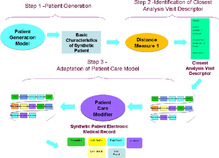
Our method has three major steps (Figure 1). The first is the creation of a population of synthetic patients. The illnesses and injuries of the synthetic patients should mimic, in as many verifiable ways as possible, those present in the real data.

Figure 1.

The Generation process for synthetic electronic medical records.

The second step is identification of the medical care that each of the synthetic patients would receive, based on the model present in the real data.

The third step is the adaptation of the care models from the real data to the synthetic patient population. Currently, this is the least automated of all the steps, but one for which we hope to further automate as results from the initial set of synthetic records are analyzed.

2.2. Step One: Creation of the population of synthetic patients

The first step, creation of the population of synthetic patients, has many smaller steps, but begins with the variables that drive the patient visit records. We will discuss the merits and drawbacks of the EMR variables available to drive the creation of the synthetic patients and describe the patient synthesis procedure.

2.2.1. Choice of the Driving Variable

There are many possible variables, such as syndrome, sub-syndrome [20], chief complaint, or diagnosis codes that can be identified as the variable to reproduce first, thus to drive, the synthetic patient population. In the data set of real EMRs, the fidelity of the data as well as the quality influenced the decision for which variables to drive the synthetic population. From the set of pilot records in the 4–11 age groups, we see in Table 1 that the final diagnosis is the least likely missing datum in the set of records. Thus keying the synthetic population off the final diagnosis ICD-9 codes would allow us to use the largest number of real records in our computation of distributions.

Table 1.

Missing fields in the data set.

Datum	% of visits missing in real data
Chief Complaint or Reason for Visit	14.84
Sub-syndrome	16.48
Syndrome	45.59
Final diagnosis ICD-9 code	.28

The quality of the driving variable as well as the quantity of real records is also a factor in the decision to use final diagnosis ICD-9 codes as the driving variable. If we consider first the use of sub-syndromes (omitted in about 16% of records), we note the projection of disease or injury to sub-syndrome is many-to-one, thus, there are many illnesses or injuries that yield the same sub-syndrome in the medical record. The purpose of the records is to reproduce the attributes in the original records. However, if the sub-syndromes were used as the basis or the “driving” variable for the synthetic patients, each synthetic patient must be matched to likely models of care. For example, for the sub-syndrome ‘injury’, a care model could include anything from that for a head laceration to that for multiple fractures. In order to both represent the range of injuries and arrive at a relatively specific pattern of care, diagnoses would need to be assigned to the syndromes. Otherwise, any algorithm that matches synthetic patients to care models would be quite inexact. There would have to be significant post-processing of records to insure that a representative sampling of likely injuries for this age group was present in the synthetic patients’ records. Because another goal of this project is to automate as many steps as possible in the construction of the synthetic records, adding post-processing steps is undesirable. Keying the choice of diagnosis codes to sub-syndromes would also unfortunately destroy some of the time-dependence (e.g., seasonal or day-of-week effects) of some illnesses and injuries; the time dependence would be inherited from that of the sub-syndrome.

The mapping from illness or injury to syndrome assigns an even larger set of illnesses or injuries to each syndrome. Thus, the assignment of patterns of care would include many models that are quite different from each other. In addition, the syndrome is the most likely datum to be omitted in the set of real records; nearly half of the real records do not include a syndrome classification. There is also some evidence that reconstruction of syndromic time series is somewhat less robust ([21]) than reconstruction of even aggregated time series of final diagnosis codes.

Chief complaints are currently widely used as indicators in bio-surveillance because of their availability. In the bio-surveillance setting, fluctuations in particular chief complaints such as rash or fever mirror rises in the corresponding rates of infectious disease with those symptoms. Notwithstanding the importance of chief complaints in the bio-surveillance setting, we note several characteristics of chief complaints (or reasons-for-visit in outpatient data) that cause them to be a less desirable driving variable for the creation of synthetic records.

Because chief complaints are free text, an additional step of a natural language processor must be used to tease a consistent set of data from the chief complaints or reasons-for-visit. In data set, this datum was missing in approximately 15% of records. Chief complaints briefly describe the patient’s reason for the visit, but are often inexact and may not adequately or accurately describe the illness or injury. In data set, for example, there were approximately 20 different final diagnosis ICD-9 codes for the one chief complaint, the exact text ‘SORE THROAT.’ Other variations of this text, including misspellings and abbreviations, also appear and add to the inexact mapping of health state to the textual chief complaints (emergency (ER) records) or reasons-for-visit (outpatient records) that appear in the data. This is not as critical in the bio-surveillance setting, where sensitivity to change is more important than specificity of the exact illnesses that are causing the change. However, here the intent is to produce a synthetic background population that mimics the illness and injury timelines and incidences in the real population. Searching for models of care that match particular chief complaints is likely to require significant post-processing to reproduce both sufficient and necessary variation in the synthetic patients. We also note that using a free text field to drive synthetic records may be prone to over-fitting. A natural language processor would be necessary to standardize the chief complaints so they become a search-able field. Some method for inserting random typographical or grammatical errors in the final synthetic records would also be required.

Thus, the first final diagnosis ICD-9 codes, although known to be an inexact match for the exact health states of the patients (see, e.g. [22], [23] and references therein) are used as the driving data for the synthetic patients. We use the term “driver” in sense that the synthetic patients are chosen as blank slates, but assigned a final diagnosis ICD-9 according to parameters present in the real data. We then compile statistics for patient demographics and additional ICD-9 codes based on this first assigned ICD-9. This produces a set of data with the same statistical and time-dependent qualities, but with different identities of individuals.

2.2.2. Timeline Synthesis

To start the synthesis process, we begin by analyzing the timelines for the final ICD-9s in the real data. We sorted the final diagnosis ICD-9 codes from the first visit for each patient in the real data set in numeric, then alphabetic order for each patient in the real data set. The initial construction of synthetic patients is for the first visit only; the procedure for subsequent visits for a subset of the patients is explained later in the text. We truncated the ICD-9’s to three digits (for codes that do not begin with E) or four digits (for codes that begin with E), and sorted the visit records by time. We then compiled time series of each of these first final diagnosis truncated ICD-9 codes. These separate time series of “first” ICD-9 codes will be reconstructed and the resulting diagnosis will be the basis for the synthetic patient population.

We note that this particular set of data did not specify which of the ICD-9 codes the “primary” diagnoses were and which were secondary diagnoses. Thus, we used a sorting procedure as a convenience in order to reproduce a consistent set of patients. If primary diagnoses are available in the real data, sorting the ICD-9 codes would not be necessary; the primary diagnoses would be the driving data.

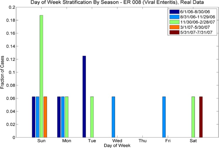
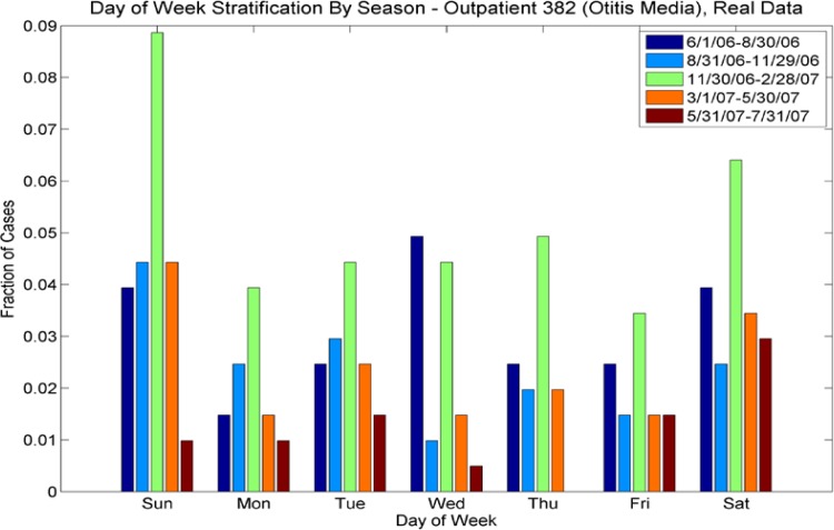
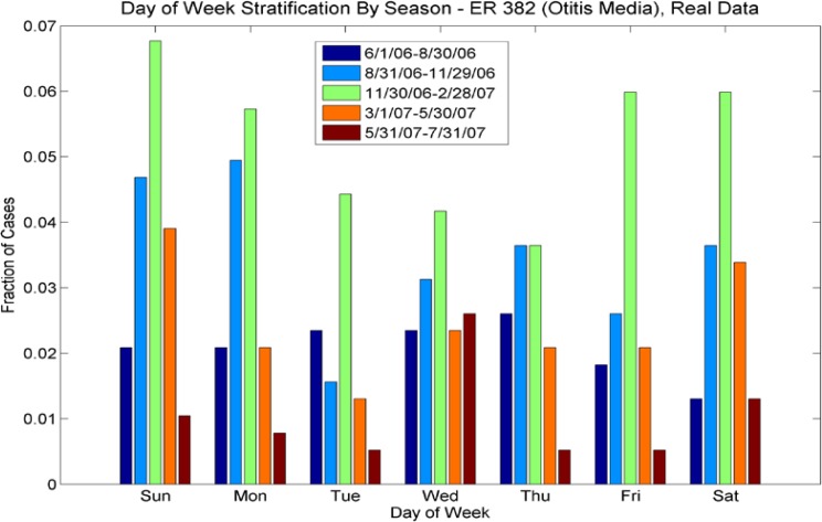
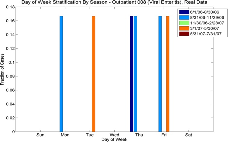
For ICD-9s with more than one case per week, we performed a wavelet reconstruction to de-noise the time series. For ICD-9s with less than one case per week, we calculated Poisson parameters for each season. We also calculated the multivariate day-of-week distribution for these sparser data sets, also varying by season. We calculated separate statistics for outpatient and emergency room (ER) cases; there are significant differences in the sparse/rich ICD-9s for ER and outpatient populations, and also significant differences in the number of cases by day of week (see Fig 2a–2d). Thus, the synthesis procedure needs to preserve the seasonal nature of the data, the day-of-week effect, and the difference between outpatient and ER cases.

Figure 2a.

Day of Week Averages by Season for ICD-9 code 008 (Viral Enteritis), ER cases from the real data. Note that the day of week varies with season – e.g. for the period 11/30/06–2/28/07(green), most cases are on Sundays, whereas for the period 8/31/06–11/30/06, cases are spread evenly among Sunday, Monday, Wednesday and Friday.

Figure 2d.

Day of Week Averages by Season for ICD-9 Code 382 (Otitis Media), outpatient cases from the real data. Note that the day-of-week effect varies for each season (by color), with different days having more pronounced numbers of cases, highly dependent on season. For example for the period 6/1/06 to 8/30/06, most cases occurred on Wednesdays, but for the period 11/30/06–2/28/07, most cases occurred on weekends. Contrast with Figure 2b, ER cases for this ICD-9; the day-of week distributions for both vary seasonally but in different ways.

Some of the ICD-9 codes have many cases per week, some have less than one. Faithful synthesis of the records requires that we reproduce day of week and seasonal effects in all data streams. Wavelet reconstructions (see, e.g. [24]) adequately reproduce all frequencies of the data. However, wavelet reconstructions work best on continuous or nearly continuous data streams (see, e.g. [24] p. 14). Thus we used wavelet reconstructions for the time series with more than one case per week. The procedure was to produce a (Haar) wavelet level 2 approximation (removing some of the noise), then to round the daily cases to the nearest whole number. This yields a new time series with similar seasonality and day of week effects and a total number of cases equal or within one or two cases of the original time series. However, we note that the smoothing provided by the level-2 wavelets insured that we did not exactly reproduce the original time series.

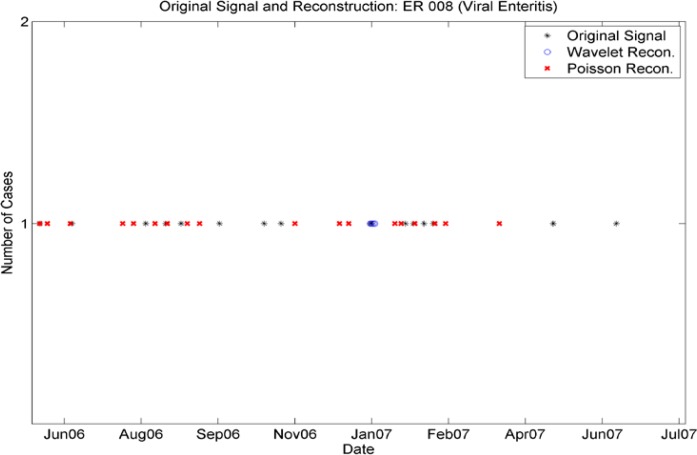
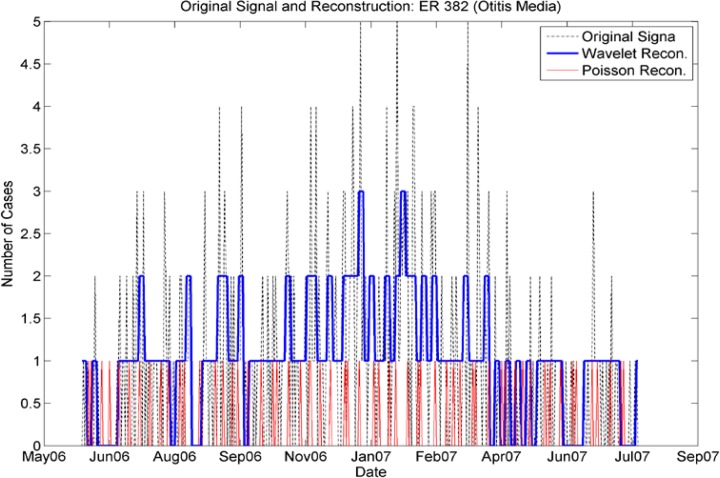
Wavelet reconstructions of isolated incidences are inadequate to reproduce low levels of cases (see figure 3a). For these low levels, the wavelet reconstruction produced fractional numbers of cases. After the rounding procedure the reconstructed time series did not match either the number of cases or the required seasonality. Figure 3a shows that there are no cases reproduced by the wavelet reconstruction in the high-incidence periods Aug 06–Sept 06 and late Jan 07–Feb 07 and only a handful of cases produced in early Jan 07, when there were few cases in the original series. In this case, the wavelet reconstruction failed to produce a realistic timeline. Thus, a different procedure is necessary for more sporadic ICD-9 data streams. For these, we find a weekly frequency that is re-calculated seasonally to adjust to differing levels in the data. In order to capture the day-of-week effect, we used a reconstruction that took a Poisson draw (against the seasonally adjusted weekly frequency) and then assigned any weekly cases according to the multivariate daily distribution present in the data for that particular truncated ICD-9 and the season. This combination of effects reproduced the statistics present in the real data but did not reproduce the time series exactly. Figure 3a shows the Poisson reconstruction (red) yields cases in the high incidence periods of Au 06–Sept 06 and late Jan 07–Feb 07 as well as sporadic cases in June 06 and Mar 07. We note that distributions of day-of-week varied not only seasonally, but also among truncated ICD-9 codes and from emergency to outpatient (Figure 2a–2d). Thus, it was insufficient to use one day-of-week distribution for all codes; they needed to be stratified by ICD-9 and by patient type (ER or outpatient).

Figure 3a.

Comparison of Wavelet Reconstruction and Seasonally Varying Poisson Reconstruction for the sporadic time series for incidence of ICD-9 008 (emergency cases). Note that the Wavelet reconstruction yields several cases in January 07, but none at other times. The Poisson Reconstruction yields sporadic cases with most frequent numbers of cases at times close to the original time series’.

In contrast, consider figure 3b. For this time series, the Poisson reconstruction (red) yielded only single cases at the times of high incidence. However, the wavelet reconstruction (blue) approximated the real time series with some smoothing of the higher peaks.

Figure 3b.

Comparison of Wavelet Reconstruction and Seasonally Varying Poisson Reconstruction for the nearly continuous time series for incidence of ICD-9 382 (Emergency cases). Note that the Poisson reconstruction failed to reproduce the time series adequately, while the wavelet reconstruction reproduced the seasonality and other variations.

We performed the wavelet reconstruction on the less sparse time series, and reconstructed the sparse time series by taking random draws from the weekly Poisson parameters, then using the multivariate distribution to assign a day of the week to the sparser time series. The net result was approximately 300 time series of cases that as a whole mimicked the distribution of cases in the real data in seasonal, day-of-week, and outbreak events. At this point, the cases are not assigned age, gender, race, ethnic group, or additional ICD-9 codes.

2.2.3. Patient Synthesis

The next procedure in the synthetic patient generation process is the assignment of patient IDs and visit IDs for each case given from the reconstructed (via either Wavelet or Poisson, for emergency or outpatient series as described above) time series. For each day in the time period defined for the synthetic patients, any cases for each reconstructed time series are designated to be a synthetic patient. For example, if on day 1, the time series for ICD-9 008 had no cases, but the time series for ICD-9 382 had 2 cases, there would be two synthetic patients constructed, each with primary ICD-9 of 382. Each synthetic patient is assigned the truncated ICD-9, a patient ID and a visit ID for that visit.

We next assign demographic information to each synthetic patient’s visit record. The distributions of gender, race, ethnic group, and age are extracted from the real data as a function of first ICD-9 code. These distributions are used to assign age, gender, race and ethnic code. We note that because race and ethnic code are jointly distributed, the original assignment of ethnic code independent of race yielded distributions that were identical as a whole to those of the original data. However, the joint race/ethnic code distributions were odd. Therefore, we readjusted our procedure to pick race and ethnic code jointly, according to the computed joint distribution found in the real data.

The next procedure in the generation of synthetic patients is the assignment of detailed ICD-9s to the patients with truncated ICD-9’s. Again, these are assigned based on the distribution in the real data.

We note that more than half of the patients in the real data had more than one final diagnosis ICD-9 code (see Table 2). Thus, the next step in patient generation is to assign multiple ICD-9 codes, again, based on the distributions found for the first ICD-9 code assigned. This is a multivariate assignment, varying seasonally. It follows the distribution for multiple ICD-9 codes based on the first sorted ICD-9 code of the first visits for patients in the real data.

Table 2.

Number of ICD-9 codes in the real data set

Number of Final Diagnosis ICD-9 Codes	% of visits in real data
0	.28
1	39.58
2	42.51
3	12.69
4	3.37
5	.85
6	.48
7	.09
8	.10
9	.01
10	.01
11	.03

The original records contain both syndrome and sub-syndrome data, although these fields are not as well populated as the first set of information (final diagnosis ICD-9 codes, age, gender, race, ethnic origin). However, we again computed the syndrome and sub-syndrome distributions based on the ICD-9 final diagnosis codes present in the real data. Because all other data in the synthetic patient records are keyed off final diagnosis ICD-9 codes, we assigned sub-syndromes based on the final diagnosis codes. Because the syndromes and sub-syndromes are assigned jointly, we keyed the syndromes off both the final diagnosis ICD-9 codes and the sub-syndromes. The existence of syndromes and sub-syndromes in the synthetic data matched the incidence in the real data.

The times-of-day of each visit are chosen according to seasonally varying multivariate distributions, computed separately for emergency and out-patients.

The last datum assigned to a patient and visit combination is the birth date of the synthetic patient, based on age. These are chosen randomly, based on age.

In the real data, about 30% of the patients had two or more visits, with some having as many as 10. In our desire to exclude any patients from the real data if their cases were unusual or they could be identified by any idiosyncrasies in their records, we truncated the number of possible visits subsequent to the first at four. Thus, each patient in the synthetic patient pool has at most 5 visits. This group included more than 99% of the patients in the real data. One or two visits were certainly the norm rather than the exception (see Table 3). We assigned numbers of visits again keyed off the first final diagnosis ICD-9 code. The time of the subsequent visits was drawn from a distribution dependent on the synthetic patient’s first ICD-9 code. The ICD-9s for subsequent visits were chosen from the distribution found in the data, with repeated visits with the same ICD-9 codes slightly more likely than repeated visits with different ICD-9 codes. Since these were subsequent visits for the already created synthetic patients, demographic information was copied and age was recalculated given the birth date and visit time. Time of visit was again calculated from separate distributions for emergency and outpatients, both varying seasonally.

Table 3.

Visits per patient in real data.

Number of Visits	% of patients in real data
1	84.83
2	11.61
3	2.38
4	.71
5	.29
6	.10
7	.06
8	.01
10	.01

2.3. Step Two: Identification of patient care models

The second major step of the creation of synthetic records is the identification of the medical care that each of the synthetic patients would receive. Basic characteristics of the synthetic patient (see Figure 1) are coming from the Patient Generation Model. They include for each visit the final diagnosis codes, syndromes, subsyndromes, age, gender, race and ethnic group of the synthetic patient. Next a distance measure is defined, and the closest Analysis Visit Descriptor is identified in the original data set. The information from this Analysis Visit Descriptor is given to major step 3: Adaptation of Patient Care Model. The steps mentioned need to be executed separately for each synthetic patient and each visit. These steps are described in detail in Section 2.3.2.

Before the above steps can be carried out Patient Care Models, Patient Care Descriptors, and Analysis Visit Descriptors need to be extracted from the EMR data set. This is a process that is performed only once for the whole data set. It is described in detail in section 2.3.1.

2.3.1. Extraction of Patient Care Models and Descriptors

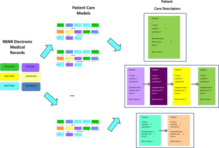
The goal of the methodology developed is to derive a care model of how the patients are treated (from the available medical records). This method has the following main steps (Figure 4):

1. Build Patient Care Models - sequences of patient care events for each patient.

2. Build Patient Care Descriptors summarizing Patient Care Models. Patient Care Descriptors are made from Analysis Visit Descriptors that summarize each visit separately.

Figure 4.

Extraction of Patient Care Models and Descriptors.

A Patient Care Model [26] is a sequence of all the health care encounters (that we will also call events) that were present in the data set for a given patient. The care model consists of up to 7 types of events: 1) analysis visit (AVisit); 2) laboratory orders; 3) laboratory results; 4) radiology orders; 5) radiology results, 6) drug (Rx) orders, 7) death event – if applicable. The events in the extracted care model are sequentially ordered based on the dates and times they occurred (present in the data).

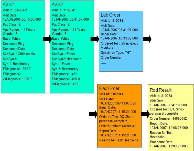
The AVisit contains the information about a given patient visit including patient’s demographic data, visit ID, visit date, working diagnoses ICD-9s, final diagnoses ICD-9s, syndromes, and sub-syndromes. The demographic data consists of patient birth date, age, race, ethnic group, and gender. Inside the laboratory orders there is information on each of the laboratory tests that were ordered during a given visit, including date and time. In the laboratory results there is information on each of the labs, with bacteria identified or information that the test was negative. Individual patient care models are of different lengths (depending on the number of visits and specific information in laboratory orders, laboratory results, radiology orders, radiology results and Rx orders). People who came only once and did not have any laboratory or radiology orders, have patient care models with one record. People who came many times and had many laboratory or radiology orders and results, have very lengthy care models (hundreds of records). Fig. 5 shows the Patient Care Model for a 4–11 year old girl with two AVisits, one laboratory test (for Strep), one radiology test (DX Sinus paranasal complete) and one radiology result (DX Sinus paranasal complete).

Figure 5.

Example of Patient Care Model

The next step is to build the patient care descriptors which summarize patient care models. For each patient care model, one patient care descriptor is computed. The Patient Care Descriptor consists of Analysis Visit Descriptors (see Table 4) that describe a given visit in detail, including any laboratory and radiology tests related to that visit. If a given patient (like the one from Figure 5) had two visits, his Patient Care Descriptor will consist of two Analysis Visit Descriptors.

Table 4.

Example Analysis Visit Descriptor (for visit 3102841).

Visit Id	3102841
Visit Date	12AUG2006:20:15:00.000
Patient Class	E
Age Range	4–11 Years
Gender	F
Race	White
Ethnic Group	Not Hispanic or Latino
Deceased Flag
Deceased Date
Syndrome 1	Fever
Syndrome 2	Respiratory
…	…
Subsyndrome 1	Fever
Subsyndrome 2	Headache
…	…
Working Diagnosis 1	462
Working Diagnosis 2
…
Final Diagnosis 1	462
Final Diagnosis 2	465.9
…
Number Laboratory Orders	1
Number Laboratory Results
Number Radiology Orders	1
Number Radiology Results	1
Number Rx Orders
Botulism Like
Fever	1
…
Respiratory	1
…
Abdominal pain
Abdominal cramps
…
Headache	1
…
Blood Culture
MRSA Culture
…
Urine Culture
DX Chest
DX Sinus Paranasal	2

Each Analysis Visit Descriptor has attributes specifying the number of laboratory orders related to a given visit, specific laboratory order types (e.g., blood culture, respiratory culture, urine culture, Aerobic Culture/Smear, Platelet Auto AB), microorganisms identified (e.g., Enterobacter Cloacae, Pseudomonas Aeruginosa, Staphylococcus Aureus, MRSA), types of radiology orders (e.g., DX Chest, PX Chest, DX Abdomen, DX Sinus Paranasal), syndromes (e.g., Fever, Gastrointestinal, Severe Illness or Death), sub-syndromes (e.g., malaise and fatigue, myalgia, upper respiratory infections), working diagnoses ICD-9s, and final diagnosis ICD-9s.

The values of all the attributes mentioned so far are integer numbers, depicting how many times a given syndrome / sub-syndrome / laboratory test occurred in a given visit. For a given patient, many attributes have a value of zero. Textual attributes include patient’s race, ethnic group, and age group (0–3, 4–11, 12–19, 20–49, 50+).

The process of building descriptors is completely data driven: if there are n different microorganisms identified in the data set, there will be n corresponding fields in the descriptor; if there are m different types of laboratory tests in the data set, there will be m corresponding attributes in the descriptor.

We extracted 12318 visit records that belong to the age group 4-11 years old from the full data set. The rest of this research is performed on this data set. To reduce the sparseness of the data set, we collapsed over 2300 features into 887 features in case of boys, and into 822 in case of girls. This was performed by adding the values of similar attributes together. As an example, the attribute DX-C-Spine was created as the sum of the following features: DX-C-Spine-1-View, DX-C-Spine-2-View, DX-C-Spine-2-or-3-Views, DX-C-Spine-4-View-Min, DX-C-Spine-4-View-and-Flex-and-E, DX-C-Spine-Flex-and-Ext-Only, DX-C-Spine-Multi-View-NR, which are different types of spine X-rays. Also working and final diagnoses ICD-9s were collapsed to the first 3 digits in case of E codes, and 4 digits in other cases.

2.3.2. Identification of Closest Analysis Visit Descriptors

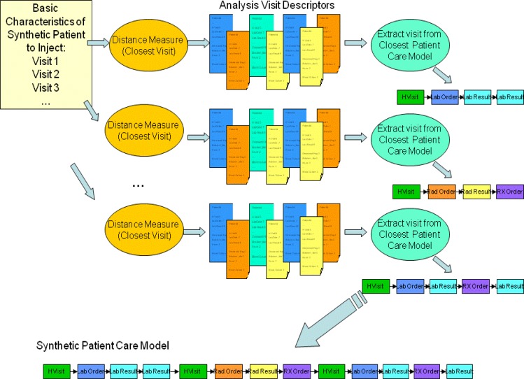
The steps described in this section are performed for every synthetic visit of every synthetic patient. The goal is to find, for each synthetic visit, a visit that is as similar as possible in the real data. Figure 6 depicts how the closest analysis visit descriptor to a synthetic visit descriptor is determined. The basic characteristics of the synthetic patient, in form of information about synthetic visits for a given patient are produced by Patient Generation Model (see Figure 1). Each synthetic visit is characterized by final diagnosis codes, syndromes, sub-syndromes, age, gender, race and ethnic group of the synthetic patient. A distance (the distance measure used is described further in this section) is computed between a given synthetic visit and all the analysis visit descriptors. A set of closest (i.e. minimum distance) analysis visit descriptors is identified. All the information about that visit is extracted from the corresponding Patient Care Model.

Figure 6.

Identification of closest analysis visit descriptor to a synthetic visit descriptor.

We have defined a distance measure between a synthetic visit and an analysis visit descriptor. This distance measure is a combination of weighted Euclidean distance and Jaccard distance [26]. Jaccard index (coefficient) measures similarity between two sets, and is defined as the size of the intersection divided by the size of the union of the sets:

$$J(A,B)=\frac{|A\cap B|}{|A\cup B|}$$

Jaccard index is a useful measure of similarity in case of sets with binary attributes. If two sets, A and B, have n attributes each, then Jaccard coefficient measures the attribute overlap that A and B share. Jaccard distance is defined as:

$$J_{\mathit{dist}}(A,B)=1-J(A,B)=\frac{|A\cup B|-|A\cap B|}{|A\cup B|}$$

We defined and used the following distance measure to identify the closest Analysis Visit Descriptor to a given synthetic visit descriptor:

$$\mathit{dist}(A,S)=J_{\mathit{dist}}(A,S)+\frac{E_{\mathit{dist}}(A,S)}{70}$$

where A stands for Analysis Visit Descriptor, S – for Synthetic Visit descriptor, and E_dist – for Euclidean distance. Euclidean distance is only computed on the age, and Jaccard distance is computed on the remaining attributes: truncated final diagnosis codes, syndromes, and subsyndromes.

2.3.3. Choice of Best Care Model

The last step in this process is choosing a care model from among those analysis visit descriptors identified as closest. Because the analysis visit descriptors were chosen using only the first 3 or 4 digits of the final diagnosis ICD-9 code, there can be slight discrepancies between details in the descriptors and in the synthetic patient’s visit record. To find the closest records, we employ an assignment algorithm to examine details. If among those identified by the previous step, a descriptor exists that exactly matches the final diagnosis ICD-9 code or codes (all digits) then that descriptor is listed as preferred by the assignment algorithm. If more than one such descriptor exists, then a descriptor is chosen randomly from among these. If no such descriptor exists, the algorithm looks for the most matches of final diagnosis ICD-9s. If more than one such descriptor exists, again, a random choice is made. If no analysis visit descriptors are singled out as being more suitable than others, a random selection is made by the assignment algorithm.

2.4. Step Three: Adaptation of health care models to each synthetic patient

The last step of the process, the adaptation of care models to the individual synthetic patients, begins with the selection of the care model that most closely matches the synthetic patient. The analysis visit descriptor is selected as described in the previous paragraph. The care models that are identified in the selected analysis visit descriptors are extracted from the data set. All the selected care models are sanitized, meaning that any textual references to dates, clinicians’ names, hospitals, particular events or specific patients are removed while maintaining the meaning of the text. This is especially applicable to radiology and laboratory results. The intervals between dates and times of care events in the care models are preserved so they can be reproduced (with noise) in the synthetic patients.

The first procedure in the adaptation of the care models is the identification of the particular care model and the records contained in it. The chief complaint (or reason for visit in outpatient records) and working diagnoses are reproduced, while maintaining the final diagnosis codes in the synthetic patient visit record. Diagnoses, sub-syndrome, and syndrome summaries are constructed from the information in the synthetic patient visit record, but chief complaint and working diagnoses are taken from information in the care model. Any laboratory orders or radiology orders are assigned identification numbers according to the model present in the data, but using fictitious actual numbers. These numbers are kept in a table so they can be repeated on the corresponding laboratory and/or radiology results. The laboratory and radiology order tables are constructed for each synthetic patient according to the pattern in the care model. The last step is the construction of any laboratory or radiology results according to the pattern in the care model. All dates in the synthetic record are based on the synthetic patient visit record’s date and time. The time intervals in the model record are used, along with an up to one hour random variation added or subtracted.

The end result of this procedure is a set of patient visit records, clinical activity records, laboratory and radiology orders and laboratory and radiology results for the entire set of synthetic patients. The patterns of care for each set of final diagnosis ICD-9 are repeated in the synthetic patients. The timelines for each ICD-9 were reconstructed so the properties in the original data set were preserved.

3. Results

3.1. Validation Overview

We validated the synthetic electronic medical records in two ways. The intent of the project was to produce a data set that can be used as a stand-in for real electronic medical records in algorithm testing. We are concerned with verifying the synthetic data exhibited the same seasonality, day-of-week effects, demographic distributions, and distribution of cases as the real data. However, the aggregate data could exhibit all these properties consistent with the real data set and be inconsistent with what is expected for the model of care for any specific patient. Thus, we also examined each of the constituent files for inconsistencies across a synthetic individual’s record, and to make sure the care for a particular ICD-9 or set of ICD-9’s matched an expected care model. We will describe the validation of properties across the entire data set and across the individual synthetic records.

3.2. Aggregate Data Set Validation

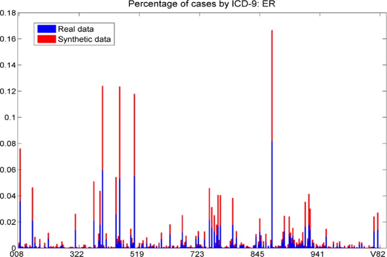
The distribution of final diagnosis ICD-9s for the original data set and for the set of synthetic records that reproduced 30% of the real records (hereafter, the “synthetic data set”) is shown in figures 7a and 7b. It is not surprising that the distribution of cases across ICD-9s is reproduced since the individual visits were taken from each ICD-9’s time series. However, the verification of this fact is important.

Figure 7a.

The fraction of each ICD-9 in the real and synthetic data sets, ER cases. We note that the distribution of cases across ICD-9s is similar in the real and synthetic data sets; each bar shows approximately the same area for the red (synthetic) and blue (real) data.

Figure 7b.

The fraction of each ICD-9 in the real and synthetic data sets, outpatient cases. We note that the distribution of cases across ICD-9s is similar in the real and synthetic data sets. Each individual bar shows approximately the same area for the red (synthetic) and blue (real) data.

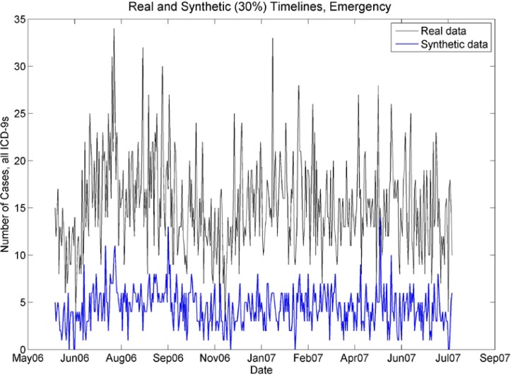
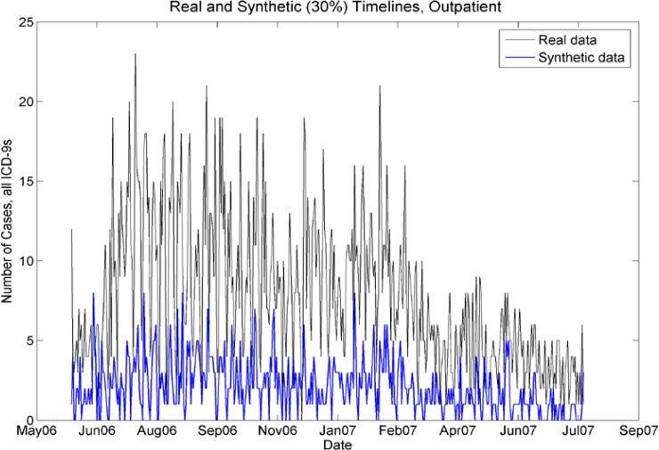
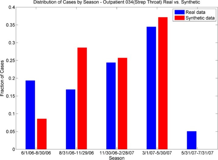
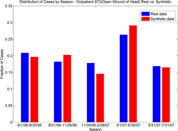
It is important that any synthetic data set as a whole mimics the timeline of the original data set. Although each constituent ICD-9 timeline was reproduced, it is not assured that the seasonality of the all cases would be preserved. Figures 8a and 8b show that although the synthetic data set has lower case counts, the peaks in the numbers of cases follow the same model as the real data set when the case counts are aggregated. Figures 9a and 9b are representative of the comparisons of seasonal differences for individual ICD-9s. We see that the seasonal distributions are reproduced in the synthetic data.

Figure 8a.

Real and synthetic timelines for emergency cases. Note that although the synthetic case counts are 30% of the case counts in the real data, the seasonality is preserved. In particular, note the peaks in July 06, late August 06, Jan07–March 07, and lower case counts in November 2006.

Figure 8b.

Real and synthetic timelines for outpatient cases. Although the synthetic case counts are 30% of the real case counts, the seasonality is preserved. In particular, note the peaks in July–Aug 06, Jan/Feb 07, and the drop-off of cases from April 07 to July 07.

Figures 9a and 9b.

Distribution of Cases by Season. The outpatient plot (top) shows the seasonal distributions of ICD-9 034 (strep throat) for real data are echoed in the synthetic data; the ER plot (bottom) shows the different seasonal distribution for ICD-9 873 (open wound of head) are echoed in the synthetic data.

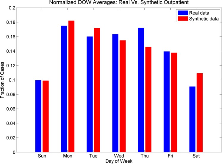
The day-of-week distribution for the aggregated cases is shown in figures 10a and 10b. We see that the day-of-week distributions for the synthetic data set of ER cases do not have a pronounced effect on Sundays, but do show a pronounced effect for Saturdays. The lower fraction of cases on Wednesday, Thursdays and Fridays is also reproduced. The day-of-week effect for the outpatient cases was mimicked more closely; we see a much smaller fraction of cases on weekends in both the real and the synthetic data sets, and more cases in the beginning of the week than at the end of the week.

Figure 10a:

The fractions of cases for each day of the week for both real and synthetic cases for ER patients and 10b: The fractions of cases for each day of the week for both real and synthetic cases for outpatients. For ER cases, we note the higher numbers of cases on Saturday and Sunday, although in this figure the Sunday counts are not as elevated in the synthetic data as in the real data. However, the drop in cases on Wednesdays, Thursdays, and Fridays and peak in cases on Saturdays are reproduced. For outpatients, we note the lower fractions of cases on weekends, and elevated numbers of cases on Mondays. However, the higher fraction of cases on Thursdays is not reproduced as well in the synthetic data set.

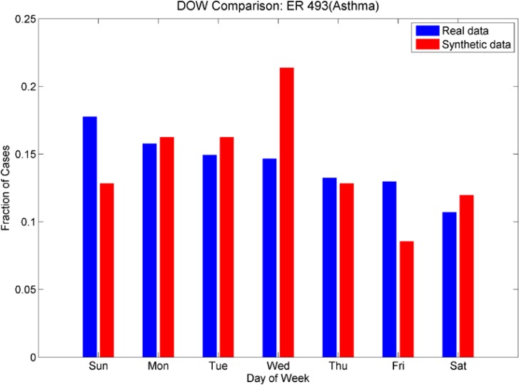
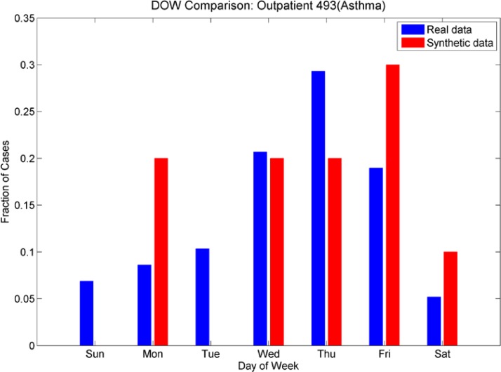
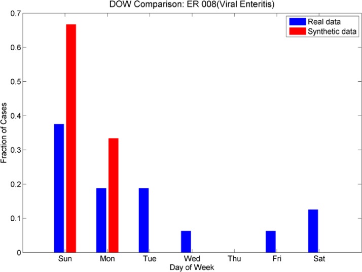
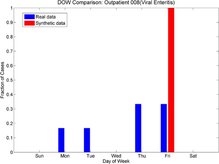
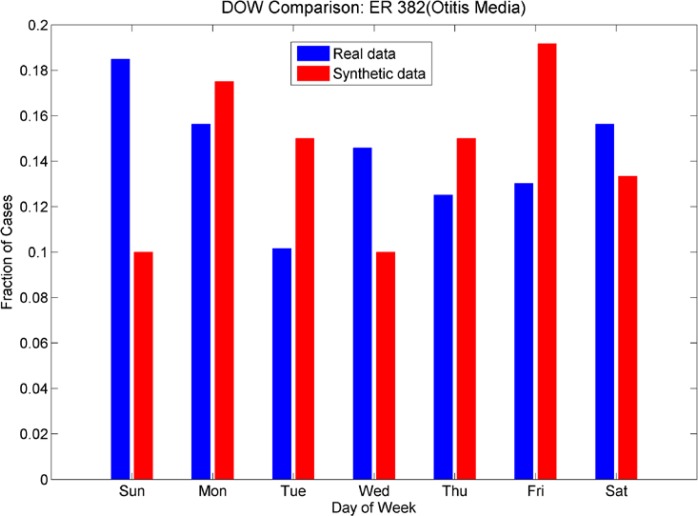
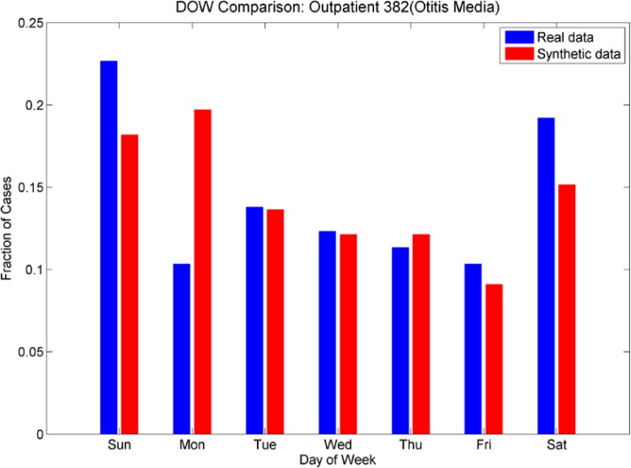
We also investigated day-of-week effects for individual ICD-9’s. Looking at Figures 11a and 11b (day of week effects for ICD-9 493, asthma), note that the outpatient plot shows more cases at the end of the week than at the beginning and this effect is reversed in the ER plot (more cases at the beginning of the week than at the end). These effects are mimicked in the synthetic data sets. Figures 12a and 12b show the day-of-week effects for ICD-9 008 (viral enteritis). The ER and Outpatient cases again show differences in the distribution of cases in the beginning and end of the week. This ICD-9 is a sparser time series, thus we expect that with the 30% reduction in cases for the synthetic data set, there will be days that do not have cases. We see, however, that the increased number of cases at the beginning of the week for ER and the end of the week for outpatient are again mimicked in the synthetic data. Figures 13a and 13b show the day-of-week distributions for ICD-9 382 (Otitis Media). The Outpatient data shows a pronounced increase in cases on the weekends; this is successfully mimicked in the synthetic data, although there are more cases on Mondays in the synthetic data than in the real data. The ER plot shows a different day-of-week distribution in the real data. This effect does not show the usual increased activity on weekends as with some other ICD-9s and instead oscillates irregularly. The synthetic data, on the other hand, oscillates more regularly, showing a somewhat bimodal distribution across the week. We note that this ICD-9 was one of the richer data sets. It is possible that the wavelet reconstruction smoothed the irregular oscillation present in the real data, but this hypothesis was not investigated at this time.

Figures 11a and 11b.

Day-of-week comparison for ICD-9 493 (Asthma). The outpatient time series are sparse, the ER time series are not. The outpatient plot shows an increased number of cases at the end of the week, the ER plot shows an increased number of cases at the beginning of the week. The synthetic data sets mimic this effect, although we note a higher number of cases that were expected on Wednesdays in the synthetic ER data set.

Figures 12a and 12b,

Day-of-week comparison for ICD-9 008 (Viral Enteritis). These are sparse time series in both emergency and outpatient. The ER plot shows an increased number cases at the beginning of the week for both real and synthetic, while the Outpatient plot shows an increased number of cases at the end of the week. The synthetic data sets mimic this effect.

Figures 13a and 13b.

Day-of-week comparison for ICD-9 382 (Otitis Media). The outpatient plot shows that the increased number of cases on weekends was mimicked by the synthetic data set, although there is an unexpected increase in cases on Mondays for the synthetic data. The day-of-week effect is not as pronounced in the ER data; the synthetic data do not mimic it as successfully.

The demographic test for goodness of fit was performed using a Kolmogorov-Smirnov test for identical distributions. For all variables, the null hypothesis that the distributions were identical was not rejected and the p-values were quite large, indicating there is little evidence that the distributions for all demographic variables for the synthetic data and for the real data are different. The results for the synthetic data set are indicated in table 6.

Table 6.

Results of Kolmogorov-Smirnov test for identical distributions. High p-values indicate that the null hypothesis (the distributions are equal) is unlikely to be false.

Demographic Variable	P-Value, ER Data	P-value, Outpatient Data.
Gender	1.0	.9870
Age	.8420	.9798
Race	.9973	.7344
Ethnic Group	.2739	1.0

The number of visits per synthetic patient is shown in table 7. These compare to the figures in table 3 for the real data. Similarly, the number of final diagnosis codes per synthetic patient (table 8) is comparable to the number of final diagnosis codes per patient in the real data (table 2). We note that slight differences in both of these measurements are both expected and desirable to insure that we did not over-fit the synthetic data.

Table 7.

Number of Visits per Patient in Synthetic Data

Number of Visits Per Patient	Number of Patients	Percent of Patients
1	2388	85.05%
2	334	12.15%
3	49	1.78%
4	23	.84%
5	5	.18%

Table 8.

Number of Final Diagnosis Codes per Visit in Synthetic Data

Number of Final Diagnosis Codes per Patient Visit	Number of Patient Visits	Percent of Visits
1	1100	33.64%
2	1690	51.68%
3	401	12.26%
4	68	2.08%
5	11	.34%

3.3. Individual Record Validation

Because the care models were chosen based on the truncated (3 or 4 digit ICD-9’s) we note that some discrepancies between final diagnosis and care model invariably occurred when the exact match for ICD 9’s could not be found in the data. The percentage of such records is listed in table 7. However, we note that the process of identifying these records and flagging them for adjustment is relatively straightforward. For example, a synthetic patient with an ICD-9 for insect bite was assigned a care model for a dog bite. The information in the record required alteration, using expert opinion, to that for the diagnosis in the synthetic patient’s record.

A subject matter expert reviewed the synthetic medical records to look for anomalies and inconsistencies in the format and content of the records. We sorted anomalies into 5 categories. The first category is a mismatch between information in the record which would indicate a mismatch of care model to synthetic patient. The second category is incompatible ICD-9 codes, indicating subtle problems with the algorithms that assign multiple ICD-9 codes to patients. The third category is the assignment of ICD-9 codes that are not appropriate either for the gender or the age of the patient. The fourth category is the assignment of syndromes or sub-syndromes that seemed unusual, given the synthetic patient’s final diagnosis codes, and the fifth category was typographical or formatting errors in the synthetic records. All anomalous records were investigated. The anomalies appear in table 3.

Because the care models were chosen based on the summary (3- or 4-code) ICD-9 codes, we expected that there would be some mismatch of chief complaint or exact ICD-9 of the care model to the synthetic patient. This was somewhat mitigated by the identification of exact ICD-9 codes of the care model with exact ICD-9 codes of the synthetic patient when there were multiple identified care models. The incidence of ICD-9/chief complaint mismatch was less than 1%, or 27/3272 records. These errors were a mixture of animal bites that did not match the ICD-9 code (typically the ICD-9 for the synthetic patient was an insect bite and the care model assigned was for a dog bite) and injuries to extremities that did not match the ICD-9 codes of the synthetic patients (e.g. an ICD-9 for a finger injury and a care model for a toe injury). Some of these anomalies can be addressed algorithmically, by automatically flagging records that did not have an exact ICD-9 match for the care model. In those cases, care models would have to be synthesized using expert opinion if they were not present in the data; this has been done previously for cases of tularemia for which there were no cases present in the data (see [21]).

We also identified inconsistencies in the assignment of multiple ICD-9 codes. In 7/3272 cases, the mutually exclusive ICD-9 codes of 787.01(nausea with vomiting) and 787.03 (vomiting alone) were assigned to some synthetic patients. This error can be corrected with an algorithm adjustment to disallow assignment of mutually exclusive ICD-9 codes.

Although there were a significant number of synthetic records flagged because of possible anomalies in the assignment of syndromes and sub-syndromes, we note that after investigation, few of these records were truly anomalous. Because syndromes and sub-syndromes are often assigned based on chief complaints and working diagnoses, in the real data there are significant variations in these assignments even for a single final diagnosis ICD-9. Thus, many of the syndrome or sub-syndrome assignments that were flagged as strange, mismatched, or incongruous were syndrome/ICD-9 or subsyndrome/ICD-9 assignments that exist in the real data. The incidence of possible anomalous syndrome or sub-syndrome assignments was 24/3272, while the syndrome or sub-syndrome assignments that, after investigation, proved to be suspect were 4/3272. This does not include possible erroneous syndrome or sub-syndrome assignments due to a mismatch between identified care model and synthetic patient ICD-9 (already identified as errors). There were 4/3272 such records. Because many cases in the first category of errors include injuries, the syndrome and sub-syndrome assignments were in line with ICD-9 codes even if the exact care model/synthetic patient ICD-9 codes did not match.

Review of the radiology orders/results table yielded additional inconsistencies. There were 54 additional suspected inconsistencies between ICD-9 and radiology orders; they were all due to mismatch of care model details to synthetic patient details (error category A). After investigation, 13 of these were found to be unusual, but not totally unexpected patterns of care existing in the real data, and 1 was dismissed as a coding error in the real data. Thus, 40 additional errors were added to group A.

After review of the laboratory orders and results table we found 11 suspected errors. One was a suspected typographical error (a laboratory order was listed twice when no laboratory result existed in the care model) and 3 were found to be care model mismatches.

We note that the possible anomalies that were noted after expert review were 141/3272 records, and the anomalous synthetic patient records that, after investigation and verification, require an algorithm change or record adjustment, were 91/3272. This corresponds to an error rate of less than 3% (see table 9).

Table 9.

Error Types and Incidence (out of 3272 visit records). Percent Flagged and Verified are calculated based on the total number of synthetic patient visits.

Error	Num. Flagged	Number Verified	Percent Flagged	Percent Verified
Care model mismatch	96	80	2.9%	2.4%
Incompatible ICD-9 codes	8	8	.24%	.24%
Gender or Age Mismatch	9	6	.27%	.18%
Erroneous syndrome or sub-syndrome assignment	24	4	.73%	.12%
Typographical or formatting error	5	4	.15%	.12%
Total	141	91	4.3%	2.8%

4. Discussions

The purpose of this research effort was to produce synthetic “background” electronic medical records for the population in the pilot group. An earlier research project [27], through which some of the methods for this project were developed, centered on producing electronic medical records for disease victims, based on the model present in the set of real records. We note that the simulated disease from the earlier project, tularemia, was not present in the real records. The laboratory orders, radiology orders, and disease progression for each synthetic patient were synthesized, based on values in the literature, similar illnesses in the population, and expert opinion. Certainly the injection of various illnesses or results of bio-terrorism can be injected into the synthetic background records using a procedure similar to that used for injection of tularemia.

In locations other than the United States, there are fewer privacy restrictions on the use of medical record data for research. This research project, then, may seem moot. However, this procedure can be adapted for altering a set of background medical records to match a patient population that is not present in real records. If background demographics are known but EMRs are not available, records for the known population can be synthesized using care models and EMRs from another location. The care models could be adjusted to reflect local standards of care as well. As mentioned above, the procedures can also be used to inject disease or bioterrorism victims into the background data to test bio-surveillance or preparedness algorithms.

The final aim for this research is the development of a suite of algorithms available on the public health grid. This suite of algorithms, given real electronic medical records with a range of formats as input, can produce the synthetic identities and synthetic medical records with the same properties as the original records. Although this pilot program only showed this is possible for a small set of records with a particular form, in one age group, many of the difficulties of producing the patients and reproducing a complicated set of attributes have been resolved.

The 4–11 age-group was chosen because of the simplicity of the cases and the relative lack of chronic or complicated disease in the population. For the most part, the patients in this age group get sick or injured, get treated, and get well. Some return with episodes of chronic illness such as asthma, but individuals with, e.g. congenital conditions have been purposely excluded so that no identifying characteristics in the pattern of care would suggest the identity of a real patient.

Future research must focus on more complicated synthetic patient care models. Rather than creation of visits of synthetic patients, as in this age group, synthetic patients with histories at various stages of entry into the health care system would need to be created. As in this set of data, any outliers, that is, patients that do not fall into the norm as far as combination of illnesses or care models are concerned, would need to be excluded. Several “mainstream” care models would need to be developed as hybrids of care for relatively common co-morbid conditions, e.g. diabetes and hypertension. In this way, individual differences in care models could be varied without loss of fidelity in the accuracy of the care model for any synthetic patients. Since the goal is a realistic set of medical records, including anomalies, outlier illnesses and care models can be synthesized and injected into the data in the same fashion as a tularemia outbreak was synthesized when no tularemia cases were present in the background data [27]. The end result is a set of completely synthetic records that reflects the spectra of illnesses and models-of-care but for which individual synthetic patients are not traceable to any patients in the real data set.

Figure 2b.

Day of Week Averages by Season for ICD-9 Code 382 (Otitis Media), ER cases from the real data. Note that the day-of-week effect varies for each season (by color), from little difference in relative height for each day of the week (dark blue 6/1/06 – 8/30/06 and red 5/31/07–7/31/07) to large differences in relative height for each day of the week (green 11/3/06–2/28/07, light blue 8/31/06–11/29/06 and orange 3/31/07–5/30/07). Contrast with a sparse time series (Fig. 2a).

Figure 2c.

Day of Week Averages by Season for ICD-9 code 008 (Viral Enteritis), outpatient cases from the real data. Note that there is a change from cases occurring on Monday, Thursday and Friday (light blue, 8/31/06–11/29/06) to cases occurring on Tuesdays and Fridays (3/31/07–5/30/07). Contrast with Figure 2a, for ER cases.

References

- 1.Mnatsakanyan Z, Burkom H, Coberly J, Lombardo J. Bayesian Information Fusion Networks for Biosurveillance Applicatoins. JAMIA PrePrint. 2009 Aug 28; doi: 10.1197/jamia.M2647. [DOI] [PMC free article] [PubMed] [Google Scholar]
- 2.Mnatsakanyan Z, Mollura D, Ticehurst D, Hashemian M, Hung L. Electronic Medical Record (EMR) utilization for public health surveillance. AMIA Annu. Symp. Proceed. 2008:2008_480–484. [PMC free article] [PubMed] [Google Scholar]
- 3.Klompas M, Lazarus R, Hanney G, Hou X, Daniel J, Campion F, et al. The Electronic Support for Public Health (ESP) project: automated detection and reporting of statutory notifiable diseases to public health authorities. Advances in Disease Surveillance. 2007;3:3. [Google Scholar]
- 4.Klompas M, Haney G, Church D, Lazarus R, Hou X, Platt R. Automated identification of acute hepatitis B using electronic medical record data to facilitate public health surveillance. PLoS ONE. 2008 Jul 9;3(7):e2626. doi: 10.1371/journal.pone.0002626. [DOI] [PMC free article] [PubMed] [Google Scholar]
- 5.Lazarus R, Klompas M, Campion FX, McNabb SJ, Hou X, Daniel J, Haney G, et al. Electronic Support for Public Health: validated case finding and reporting for notifiable diseases using electronic medical data. J Am Med Inform Assoc. 2009 Jan-Feb;16(1):18–24. doi: 10.1197/jamia.M2848. Epub 2008 Oct 24. [DOI] [PMC free article] [PubMed] [Google Scholar]
- 6.Almenoff J, Tonning JM, Gould AL, Szarfman A, Haugen M, Ouellet-Hellstrom R, et al. Perspectives on the use of data mining in pharmacovigilance. Drug Safety. 2005;28(11):981–1007. doi: 10.2165/00002018-200528110-00002. [DOI] [PubMed] [Google Scholar]
- 7.Wang X, Hripsak G, Markatou M, Friedman C. Active Computerized Pharmacovigilance Using Natural Language Processing, Statistics and Electronic Health Records: A Feasibility Study. JAMIA. 2009 May-Jun;16(3):328–337. doi: 10.1197/jamia.M3028. [DOI] [PMC free article] [PubMed] [Google Scholar]
- 8.Evans RS, Lloyd JF, Abouzelof RH, Taylor CW, Anderson VR, Samore MH. System-wide surveillance for clinical encounters by patients previously identified with MRSA and VRE. Stud Health Technol Inform. 2004;107(Pt. 1):212–6. [PubMed] [Google Scholar]
- 9.Himes B, Dai Y, Kohane I, Weiss S, Ramoni M. Prediction of Chronic Obstructive Pulmonary Disease (COPD) in Asthma Patients Using Electronic Medical Records. JAMIA. 2009 May-Jun;16(3):371–379. doi: 10.1197/jamia.M2846. [DOI] [PMC free article] [PubMed] [Google Scholar]
- 10.Evans RS, Wallace CJ, Lloyd JF, Taylor CW, Abouzeloft RH, et al. the CDC Prevention Epicenter Program Rapid Identificatison of hospitalized patients at high risk for MRSA Carriage. JAMIA. 2008;15(40):506–512. doi: 10.1197/jamia.M2721. [DOI] [PMC free article] [PubMed] [Google Scholar]
- 11.Bhumiratana B, Bishop M. Privacy aware of data sharing: Balancing the usability and privacy of datasets. Proc 2nd Intl Conf Perv Tech Rel Assist Envir. 2009:73. [Google Scholar]
- 12.Narayanan A, Shmatikov V. Robust de-anonymization of large sparse datasets. Proc IEEE Symp Sec Priv. 2008:111–125. [Google Scholar]
- 13.Lakshmanan LVS, Ng RT, Ramesh G. On disclosure risk analysis of anonymized itemsets in the presence of prior knowledge. Trans Knowl Discv Data. 2008;2:13. [Google Scholar]
- 14.https://www.epimodels.org/midas/about.do
- 15.Burr T, Klamann R, Michalak S, Picard R. Generation of Synthetic Biosense Data. 2005. Los Alamos National Laboratory Report LAUR-05-7841. [Google Scholar]
- 16.http://archimedesmodel.com/
- 17.The MIMIC project: http://www.projectmimic.com/
- 18.Johnson ML, Pipes L, Veldhuis PP, et al. AutoDecon, a deconvolution algorithm for identification and characterization of luteinizing hormone secretory bursts: Description and validation using synthetic data. Anal Biochem. 2008;381:8–17. doi: 10.1016/j.ab.2008.07.001. [DOI] [PMC free article] [PubMed] [Google Scholar]
- 19.Watkins RE, Eagleson S, Veenendaal B, Wright G, Plant AJ. Disease surveillance using a hidden Markov model. BMC Med Inform Decis Mak. 2009;9:39. doi: 10.1186/1472-6947-9-39. [DOI] [PMC free article] [PubMed] [Google Scholar]
- 20.CDC Biosense website: http://www.cdc.gov/BioSense/ ; definition of sub-syndromes at http://www.cdc.gov/Biosense/files/PHIN2007_SubsyndromesPresentation-08.22.2007.ppt
- 21.Moniz L, Buczak AL. Replicating Time Scales for Synthetic Medical Records. AMIA Spring Congress Proceed. 2009 [Google Scholar]
- 22.Surjan G. Questions on Validity of international classification of diseases – coded diagnoses. Int J Med Inform. 1999 May;:77–95. doi: 10.1016/s1386-5056(98)00171-3. 5492. [DOI] [PubMed] [Google Scholar]
- 23.O’Malley KJ, Cook KF, Price MD, Wildes KR, Hurdle JF, Aston CM. Measuring diagnoses: ICD-9 code accuracy. Health Serv Res. 2005 Oct;40(5 Pt 2):1620–39. doi: 10.1111/j.1475-6773.2005.00444.x. [DOI] [PMC free article] [PubMed] [Google Scholar]
- 24.Meyer Y. Wavelets and Applications SIAM. 1992 [Google Scholar]
- 25.Buczak AL, Moniz L, Feighner BH, Lombardo J. “Mining Electronic Medical Records for Patient Care Patterns”. IEEE Conference on Computational Intelligence in Data Mining; 2009. [Google Scholar]
- 26.Jaccard P. “Étude comparative de la distribution florale dans une portion des Alpes et des Jura.”. Bulletin de la Société Vaudoise des Sciences Naturelles. 1901;37:547–579. [Google Scholar]
- 27.Buczak AL, Moniz L, Copeland J, Rolka H, Lombardo J, Babin S, et al. Data-driven hybrid method for synthetic medical records generation. Proceedings of the 2008 Conference on Intelligent Data Analysis in Biomedicine and Pharmacology; pp. 81–86. [Google Scholar]