A confidence-based aberration interpretation framework for outbreak conciliation

Abstract

Health surveillance can be viewed as an ongoing systematic collection, analysis, and interpretation of data for use in planning, implementation, and evaluation of a given health system, in potentially multiple spheres (ex: animal, human, environment). As we move into a sophisticated technologically advanced era, there is a need for cost-effective and efficient health surveillance methods and systems that will rapidly identify potential bioterrorism attacks and infectious disease outbreaks. The main objective of such methods and systems would be to reduce the impact of an outbreak by enabling appropriate officials to detect it quickly and implement timely and appropriate interventions. Identifying an outbreak and/or potential bioterrorism attack days to weeks earlier than traditional surveillance methods would potentially result in a reduction in morbidity, mortality, and outbreak associated economic consequences. Proposed here is a novel framework that takes into account the relationships between aberration detection algorithms and produces an unbiased confidence measure for identification of start of an outbreak. Such a framework would enable a user and/or a system to interpret the anomaly detection results generated via multiple algorithms with some indication of confidence.

1. Introduction

Recent advances in technology have made it possible to gather, integrate, and analyze large amounts of data in real-time or near real-time. These new technologies have touched off a renaissance in public health surveillance. For the most part, the traditional purposes of health surveillance have been to monitor long-term trends in disease ecology and to guide policy decisions. With the introduction of real-time capabilities, data exchange now holds the promise of facilitating early event detection and to assist in day-to-day disease management.

With the availability of dozens of different aberration detection algorithms, it is possible, if not probable, to get different results from different algorithms when executed on the same dataset. The results of the study in [1] suggest that commonly-used algorithms for disease surveillance often do not perform well in detecting aberrations other than large and rapid increases in daily counts relative to baseline levels. A new approach, denoted here as Confidence-based Aberration Interpretation Framework (CAIF), may help address this issue in disease surveillance by using a collective approach rather than algorithm specific approach.

2. The problem statement

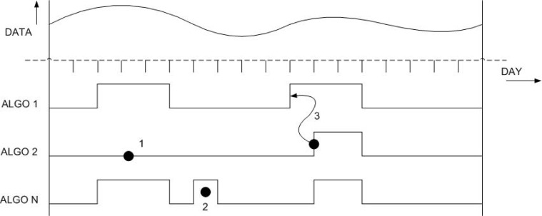
Consider a system with multiple anomaly detection algorithms as illustrated in Figure 1. Due to differences in the implementation of the algorithms and parameters used (ex: thresholds, training periods and averaging windows), the outbreak decisions may vary significantly from one algorithm to another. On the other hand, there is also a possibility that these decisions are very similar for some set of algorithms. These two extremes create a dilemma for decision makers in that there could be a situation where most of the algorithms in a system suggest an outbreak, however, not knowing the relationships between these algorithms can result in a biased decision.

Figure 1.

The Outbreak Detection Problem

As illustrated, there are three main points of concern:

• False Negative: Depending on the algorithm employed, there is a possibility of missing a real outbreak indicated as 1 in Figure 1. Obviously, this can be very damaging if the system were to make a decision based on that specific algorithm. False negatives can lead to potentially exponential damage within the general public due to delayed response to an outbreak.

• False Positive: Some algorithms are susceptible to reporting false positives, that is, detect an anomaly during peace time (indicated as 2 in Figure 1). Most systems set their anomaly detection thresholds to be as sensitive as possible to minimize the risk of missing important events, producing frequent false alarms, which may be determined to be false positives by subsequent investigation. These systems face inherent trade-offs among sensitivity, timeliness and number of false positives. False positives have a negative impact on public health surveillance because they can lead to expensive resource utilization for further investigation and can cause undue concern among the general public.

• Delayed Identification: During initial stages of an outbreak, the number of cases are on the rise and hence detecting an outbreak at this point could be very effective and potentially aid in minimizing the impact of a potential bioterrorist attack. However, depending on the algorithm(s) employed, a system may end up with some algorithms detecting outbreaks well beyond the actual start day (indicated as 3 in Figure 1). This, once again, can be very costly to public health community and impact it negatively for obvious reasons.

These three concerns result in a trade-off situations between false positives, false negatives and detection time which are typically addressed by looking at sensitivity, specificity and time to detect parameters.

In summary, a framework needs to be implemented that would enable a user/system to interpret the anomaly detection results with some indication of confidence. That is, is there a potential start of an outbreak with twenty percent confidence or is it ninety percent confidence? A framework that takes into account the relationships between algorithms and produces an unbiased confidence measure for identification of start of an outbreak is presented.

3. The proposed solution

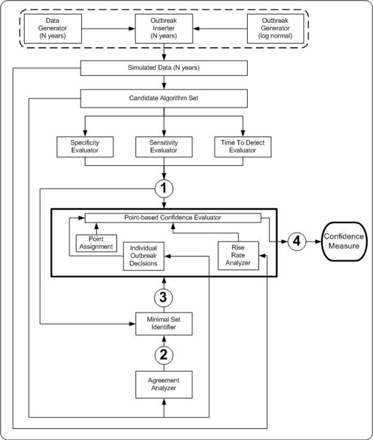
The proposed anomaly interpretation framework aims to enhance surveillance decision-making by combining results of multiple aberration detection algorithms through the use of key result metrics. Figure 2 depicts the four steps of the proposed framework and the associated linkages between them.

Figure 2.

The Confidence-based Aberration Interpretation Framework

Step 1: Specificity, Sensitivity and Time To Detect Evaluator

Traditionally, specificity and sensitivity have been used for comparing various algorithms and their performances. In this study, these two parameters are key in helping identify a subset of algorithms (referred to as minimal set) that would be sufficient to deduce an overall decision to detect start of an outbreak. The hypothesis is that the system may not require all candidate algorithms to come up with a good decision as some of them may provide redundant information.

Sensitivity of an algorithm for a given dataset is defined as the total number of outbreaks during which the algorithm flagged (at least once per outbreak) divided by the total number of outbreak periods in the dataset. Specificity of an algorithm for a given dataset, on the other hand, is defined as the total number of non-outbreak days on which the method did not flag divided by the total number of non-outbreak days in that dataset [2]:

$$\begin{array}{l}\mathit{Sensitivity}=(\mathit{True}\hspace{0.17em}\mathit{Positive}\hspace{0.17em}\mathit{Count})/(\mathit{Total}\hspace{0.17em}\mathit{Number}\hspace{0.17em}\mathit{of}\hspace{0.17em}\mathit{Outbreaks})\\ \mathit{Specificity}=(\mathit{True}\hspace{0.17em}\mathit{Negative}\hspace{0.17em}\mathit{Count})/(\mathit{Total}\hspace{0.17em}\mathit{Number}\hspace{0.17em}\mathit{of}\hspace{0.17em}\mathit{No}\hspace{0.17em}\mathit{Outbreak}\hspace{0.17em}\mathit{Days})\end{array}$$

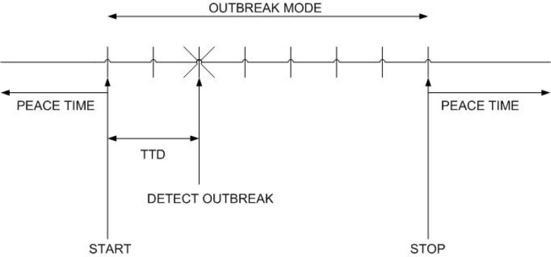
In addition to specificity and sensitivity, a third parameter called time to detection (TTD) defined as the average number of days from the first day of an outbreak until it was flagged by the algorithm, plays a vital role in the forthcoming analysis. This is a very important parameter as it aids in segregating a set of algorithms into various groups (or classes) and provides a very clear differentiation between set of algorithms based on its interpretation.

Figure 3 illustrates, in time, a progression of a sample outbreak over multiple days. Periods with no outbreaks are referred to as peace-time, while outbreak-mode refers to a time period with outbreak days.

Figure 3.

A sample outbreak

The three parameters discussed in this section provide a wealth of insight into the goal of identifying a minimal sub set of algorithms sufficient for generating an overall confidence value for an anomaly indicator.

Step 2: Agreement Analyzer

Agreement analyzer deals with quantifying the degree of agreement or relationship between any given two algorithms executed on the same data set. That is, are all candidate algorithms producing unique results? Or, is it that some algorithms yield similar results and thus provide no added value to the overall decision? This step of the framework exploits such relationship and/or agreement between any two algorithms using two quite different approaches: Correlation and Kappa Coefficient.

Correlation

Correlation is one of the most common and most useful statistics. A correlation, r, is a single number that describes the degree of linear relationship between two variables (also referred to as bivariate relationship). A positive relationship, in general terms, means that higher scores on one variable tend to be paired with higher scores on the other and that lower scores on one variable tend to be paired with lower scores on the other.

The correlation between two variables, in this case the two algorithm values or decisions, can be obtained using [3]:

$$r=\frac{N\sum xy-(\sum x)(\sum y)}{\sqrt{[N\sum x^2-{(\sum x)}^2][N\sum y^2-{(\sum y)}^2]}}$$

where x and y are the time series for daily counts, N is the total number of days in the time series, ∑xy is the sum of products of paired counts, ∑x is the sum of counts from first algorithm in the pair, ∑y is the sum of counts from second algorithm in the pair, ∑x² is the sum of squared x counts and ∑y² is the sum of squared y counts. ρ_correlation, the agreement matrix based on correlation, is obtained using the above formula as follows:

$${\rho }_{\mathit{correlation}}=\left(\begin{array}{cccc}{r}_{11}& r_{12}& \dots & r_{1n}\\ r_{21}& r_{22}& \dots & r_{2n}\\ r_{n1}& r_{n2}& \dots & r_{nn}\\ & & & \end{array}\right)$$

where r_XY is the correlation value for algorithm X against algorithm Y and n is the number of algorithms in the candidate set.

A minimum agreement threshold based on correlation $T_A^{correlation}$ needs to be defined that can be used in the next step of the framework to identify nearest neighbors for each algorithm based on the strength of the relationships.

Kappa Coefficient

An alternative approach to correlation matrix is the computation of Kappa Coefficient, which is an index that compares the agreement against that which might be expected by chance. Kappa can be thought of as the chance-corrected proportional agreement, where possible values range from +1 (perfect agreement) via 0 (no agreement above that expected by chance) to -1 (complete disagreement).

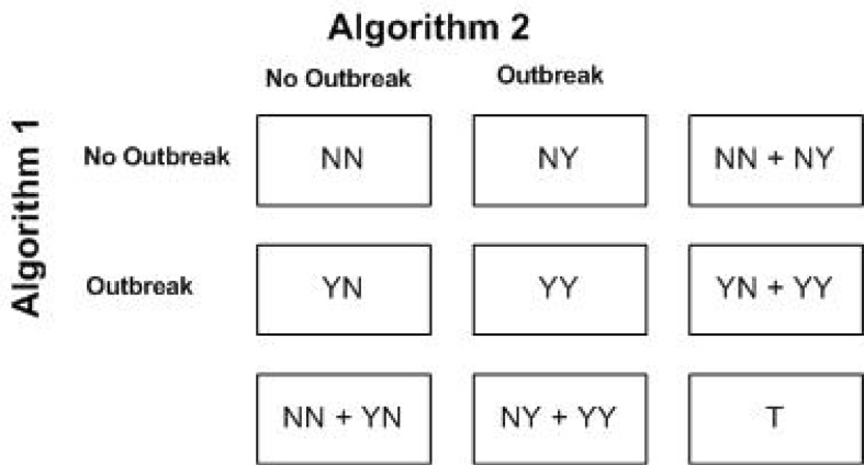
Cohen's kappa coefficient approach [4] can be used to generate kappa coefficient matrix. Consider a 2×2 table capturing decision outcomes by two different algorithms being compared as shown in Figure 4.

Figure 4.

Kappa coefficient: 2 by 2 table

The following formula was used to compute the kappa coefficient between any two algorithms:

$$\begin{array}{l}\kappa =\frac{(P_o-P_c)}{(1-P_c)}\\ P_o=\frac{NN+YY}{T},\\ P_c=\frac{NN+NY}{T}*\frac{NN+YN}{T}+\frac{NY+YY}{T}*\frac{YN+YY}{T}\end{array}$$

where P_o is the relative observed agreement and P_c is the probability that the agreement is due to chance.

_ρkappa, the agreement matrix based on kappa coefficients, is obtained using the above formulas as follows:

$${\rho }_{\mathit{kappa}}=\left(\begin{array}{cccc}{\kappa }_{11}& {\kappa }_{12}& \dots & {\kappa }_{1n}\\ {\kappa }_{21}& {\kappa }_{22}& \dots & {\kappa }_{2n}\\ {\kappa }_{n1}& {\kappa }_{n2}& \dots & {\kappa }_{nn}\\ & & & \end{array}\right)$$

where κ_XY is the kappa coefficient for algorithm X against algorithm Y and n is the number of algorithms in the candidate set.

Once the kappa matrix has been computed, it is necessary to consider the significance of obtained agreement values between any pair of algorithms. Landis and Koch [5] give the following table for interpreting the significance of the κ value. Although inexact, this table provides a useful benchmark on the significance of the above matrix.

κ	Interpretation
Negative	Poor agreement
0.0 ≤ 0.20	Slight agreement
0.21 ≤ 0.40	Fair agreement
0.41 ≤ 0.60	Moderate agreement
0.61 ≤ 0.80	Substantial agreement
0.81 ≤ 1.00	Almost perfect agreement

Based on the results and table above, the minimum agreement threshold based on kappa $T_A^{kappa}$ can be deduced, which can be set to 0.5 based on the above table. This is the value that will be used in the next step of the framework to identify nearest neighbors for each algorithm based on the strength of the relationships.

Step 3: Minimal Set Identifier

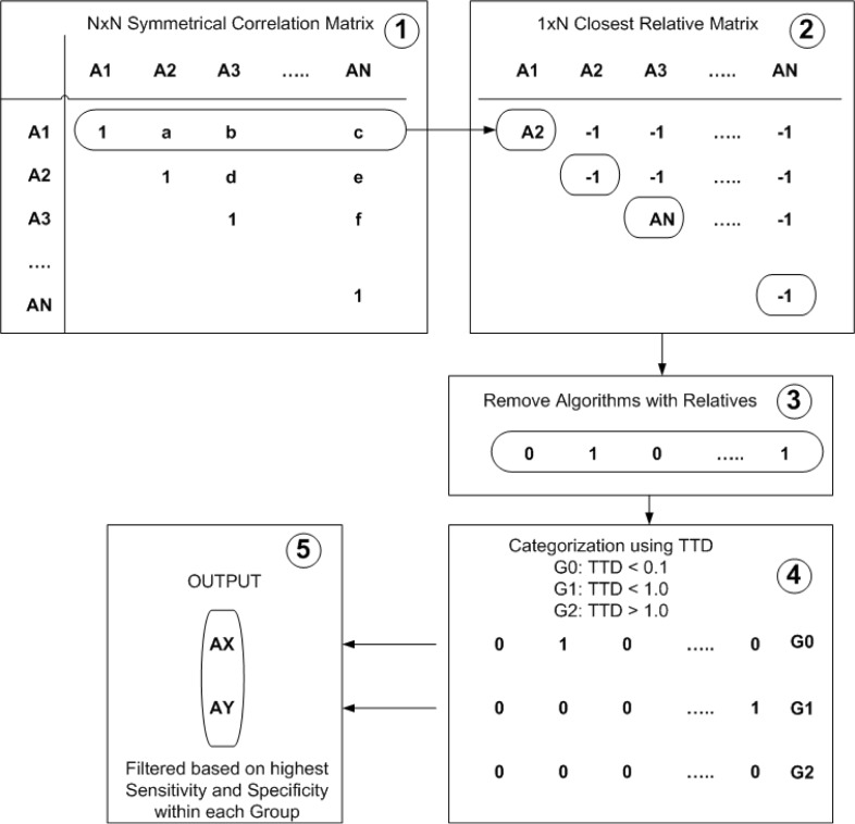
Once the sensitivity, specificity and time to detect parameters are well established for each algorithm and the agreement levels between every possible algorithm pair is known, a minimal set of algorithms can be identified that would be sufficient to produce quantifiable confidence value for the overall decision. Figure 5 illustrates a five-step process developed to identify this minimal set based on results from the previous two steps of the proposed framework.

Figure 5.

Minimal Set Identification Process

• Task 1: This task is basically setting up the agreement matrix ρ generated from Step 2 of the framework. That is, initialize ρ with computed ρ_correlation or ρ_kappa values. Note that only the upper triangle of the matrix needs to be analyzed to avoid any recursive relationships between two algorithms. That is, if A1 highly correlated to A2, then A2 is highly correlated with A1.

• Task 2: The next task deals with setting up the closest relative matrix. A closest relative to a specific algorithm X is algorithm Y that has an agreement value of at least some minimum agreement threshold (T_A) and has the highest agreement value with respect to X against all other algorithms within the set. The idea is that for each algorithm in the set, a corresponding algorithm with highest agreement value must be identified. It is entirely possible that a specific algorithm will not have a closest relative. In that case, the algorithm would be considered as an independent and thus needs to be included for next filtration task. For example, in the illustrated figure, A2 is closest relative to A1 as AN is to A3. However, algorithms A2 and AN are independent.

• Task 3: This task simply formalizes the algorithms that were selected in the previous task by removing all the algorithms from the closest relative matrix that have relatives identified, that is, the non-independent algorithms. This produces a working set of algorithms identified as 1 in the 1xN matrix.

• Task 4: The next task is to categorize the algorithms from the working set into three groups based on TTD value. The TTD was divided into three sets: close to zero days (TTD ≤ 0.1), less than one day (0.1 ≤ TTD ≤ 1.0) and greater than one day (TTD ≥ 1.0). This categorization makes intuitive sense because typically one would be interested in TTD value of less than a day. Optimally, TTD should be as close to zero as possible, but realistically, public health individuals typically identify an outbreak more than a day later.

• Task 5: Once the groups have been identified, the final task deals with identifying the minimal set of algorithms through one more stage of filtration using specificity and sensitivity values obtained from step one of the framework. This task scans through each of the groups and attempts to flag algorithms that have both highest sensitivity and highest specificity when compared to other algorithms in the same group. If one algorithm has higher sensitivity but some other algorithm has higher specificity, then both the algorithms need to be considered.

This step of the framework yields a minimal subset of candidate algorithms that have minimal relation with each other and thus, form close to an independent minimal set that would be sufficient to deduce a confidence measure for an outbreak decision for a given day.

Step 4: Point-based Confidence Evaluator

The final step of the proposed framework deals with pulling together the findings from the first three steps and working out a scheme that produces a value that corresponds to overall confidence. There are three main parameters that need to be investigated.

Parameters of Interest: Rise Rate

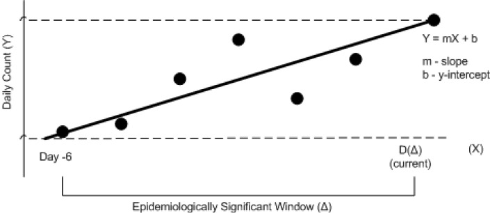
The first parameter is the rate of change (referred to as rise rate) of actual daily count values over a specific time period, which provides some basic knowledge of the positive or negative trend over the last few days and also yields the speed with which the change is occurring.

Figure 6 illustrates a typical snapshot from daily counts data where the y-axis represents daily raw count and the x-axis represents the day with D(Δ) representing the current day. The rate of change (λ) is computed using basic linear regression method [6] to define a line that fits the daily count values in best possible manner:

$$\lambda =\frac{n\sum xy-\sum x\sum y}{n\sum x^2-{(\sum x)}^2}$$

where n is the number of points being considered, x is the day and y is the count.

Figure 6.

Rise rate analysis

To be effective, the computation of rate is limited to a specific time frame referred to as an epidemiologically significant window, Δ, which is defined in number of days.

Parameters of Interest: Count Delta

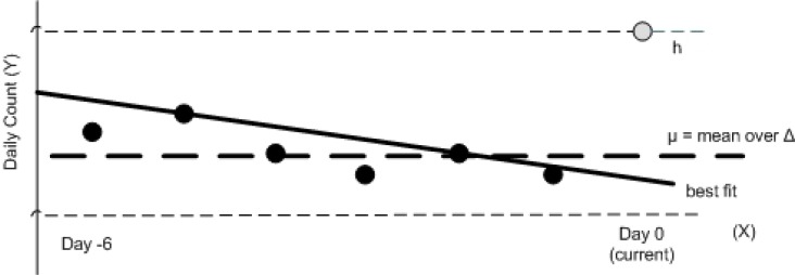
Next parameter of interest is analyzing the importance of the current day's count with respect to Δ. That is, does today's count follow a typical trend identified by the linear regression or is it drastically different and thus deserves special attention. As shown in Figure 7, there could be a scenario where past (Δ − 1) values yield a negative direction, however current day's value (h) is very high but cannot influence the linear regression formula to produce a positive slope which is more accurate in this case.

Figure 7.

Count delta

For such cases, the framework takes into account a second parameter of interest called count delta (ω). This value is simply the ratio between current day value, h, and the average value over Δ.

$$\omega =\frac{h}{\frac{1}{\mathrm{\Delta }}\sum _{i=I-\mathrm{\Delta }+1}^{i=I}{X}_i}$$

where I is the current day and X_i is the time series for daily counts.

Parameters of Interest: Outbreak Decisions

Based on the output of step three of the framework, the individual outbreak decision flags need to be considered. These provide the third parameter of interest, ϕ_i, where i refers to the algorithms in the minimal set. Each ϕ_i can have one of two values: true representing an outbreak has been detected by algorithm i and false representing no outbreak decision by algorithm i.

Point System: Rules

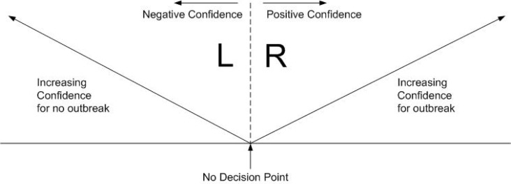
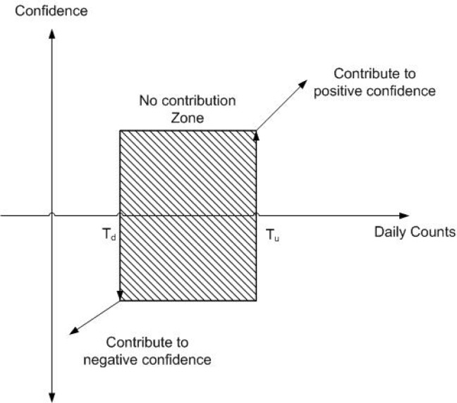
The overall objective of the framework is to produce a set of algorithms, that is as minimal as possible, to evaluate an aberration decision for any given day with some confidence value. Due to availability of multiple algorithms, a system that facilitates incremental confidence building based on contributions from various algorithms needs to be developed. A bimodal approach to confidence evaluation is proposed to address this issue as shown in Figure 8.

Figure 8.

Point assignment scheme

This bimodal approach is based on the concept of contribution to positive and negative confidence of a decision. The fundamental premise of the proposed scheme is a rule set, which is defined as the set of rules that collectively contribute to either positive or negative confidence. Positive confidence is a measure of collective strength of rules that contribute to a decision that supports identification of start of an outbreak. On the other hand, negative confidence is a measure of collective strength of rules that contribute to a decision that is against the decision of start of an outbreak. Rule sets are made of weighted combination of identified parameters of interest. Further discussion on details of rule sets will follow shortly. Once the rule set has been identified, appropriate weights (or points) are assigned to the members of the rule set contributing to either side. A set of rules that contribute to positive confidence by collective summation of all of their respective points (p) are referred to as the R set. On the contrary, a set of rules that contribute to negative confidence by collective summation of all of their respective points (n) are referred to as the L set. That is, each side adds its collective contribution followed by (p − n) to come up with overall confidence with 0 as the no decision point.

The following rules contribute to incremental positive confidence (R side rules):

$$\left[\begin{array}{cc}{\phi }_i=true& \forall i\in K\\ {\lambda }_d>T_u*{\lambda }_{d-1}& \\ {\omega }_d>T_u*{\omega }_{d-1}& \\ & \end{array}\right]$$

where d is the current day and K is the number of algorithms in the minimal set. That is, there are K + 2 rules that contribute to positive confidence with each rule having a point magnitude of p_k, where k ∈ (K+2).

The following rules contribute to incremental negative confidence (L side rules):

$$\left[\begin{array}{cc}{\phi }_i=false& \forall i\in K\\ {\lambda }_d<T_d*{\lambda }_{d-1}& \\ {\omega }_d<T_d*{\omega }_{d-1}& \\ & \end{array}\right]$$

where d is the current day and K is the number of algorithms in the minimal set. That is, there are K + 2 rules that contribute to positive confidence with each rule having a point magnitude of p_k, where k ∈ (K+2).

The use of λ and ω requires introduction of some threshold value that defines the decision points in both the upward and downward directions. Thus, the scheme makes use of T_u parameter for the positive (or upside) threshold value and T_d for the negative (or downside) threshold value. Both of these values can be computed using sophisticated approaches like neural networks, however, a simple intuitive approach using hysteresis (Figure 9) was adopted. That is, λ and ω would contribute to positive confidence if the current day values were at least T_u times bigger than the previous day values. However, they would only contribute to negative confidence if the current day values were less than T_d times previous day values. This approach assists in identifying abrupt rises and falls in the count values with respect to immediate history. The proposed rule of thumb is to use T_u ≈ 3 * T_d.

Figure 9.

Threshold hysteresis

To summarize, there are total of Z = 2(K + 2) rules that define a specific rule set ζ_i for a given point assignment i. In an attempt to simply the representation of rules and associated point assignments for L and R rules, a concise convention was designed as follows:

$${\zeta }_i=\langle 1_{L_{p1}}^{R_{p1}}{,2}_{L_{p2}}^{R_{p2}}{,3}_{L_{p3}}^{R_{p3}}{,4}_{L_{p4}}^{R_{p4}}{,5}_{L_{p5}}^{R_{p5}},\dots ,V_{L_{pV}}^{R_{pV}}\rangle$$

where numbers 1 to V represent the V (= K +2) rules, L_pV is the point assignment for the Vth Left rule and R_pV is the point assignment for the Vth Right rule.

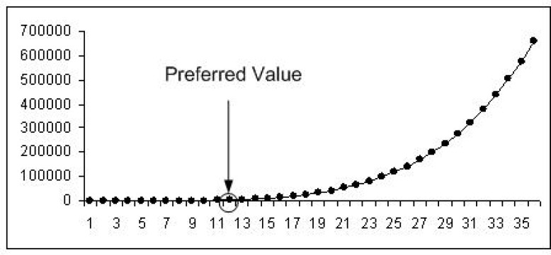
With $\frac{Z}{2}$ possible rules on each side, the most obvious choice is a balanced system with the maximum number of points for negative confidence and the maximum number of points for positive confidence to equal multiple of $\frac{Z}{2}$. That is, if both sides matched in their outcomes, then the overall confidence value would equate to 0, an indecisive line. To facilitate wider base of different points and associated effects on overall decision, a system that exercises the point assignment with an unbiased (random) allocation of points is necessary. However, before such a system can be developed, the value of maximum points for each side (M) needs to be established. This can be achieved as follows:

$$\sum _{i=1}^Z{p}_i=M$$

where p_i represents point allocation for i^th rule.

In Figure 10, x-axis represents M and y-axis represents the total number of point assignment possibilities for Z = 12 (that is, K = 6). In this specific case, M = 12 seems reasonable as it is located at the knee of the rising curve and provides 6188 assignment possibilities, a number that is quite reasonable for simulation purposes.

Figure 10.

Maximum number of points

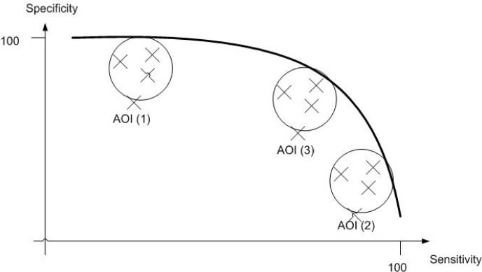
Now that the rules and point assignment method have been designed, there is a need for devising a system that interprets outcomes of the application of identified rules and associated points and yields an optimal point assignment that produces desired outcome. The proposed approach is to group sensitivty and specificity values obatined using numerous random point assignments into clusters of interest as shown in Figure 11. The idea is to identify specific areas of interest (AOI) on this scatter plot that produce outcome that is superior when compared to any single algorithm. That is, three AOIs are identified as follows: high specificity (left top); high sensitivity (bottom right) and maximum sensitivity/specificity (knee).

Figure 11.

Clusters

Any of the commonly used clustering techniques may be used to identify AOIs. The proposed approach utilizes k-means clustering [7] technique as it allows identification of initial centroids of desired clusters, which is attractive since, as discussed above, typically one would like to look at very specific clusters that provide, for instance, high specificity and high sensitivity - that is, AOI(3).

The objective of k-means approach is to minimize total intra-cluster variance, or, the squared error function:

$$V=\sum _{i=1}^k\sum _{x_j\in S_i}|x_j-{\mu }_i{|}^2$$

where there are k clusters S_i (∀i ∈ k), x_j is the sensitivity/specificity pair on the scatter plot corresponding to ζ_i and μ_i is the centroid or mean point of all the points within cluster i.

Application of clustering methodology yields a multitude of rule sets ζ_i each of which produce a sensitivty/specificity pair ν_ζi yielding:

$${\psi }_k=\left\{{\nu }_{{\zeta }_i}\right\},{\forall }_{i\in k}$$

Once ψ_k has been figured out, the idea is to then pick an appropriate rule set in a given cluster k that falls in the desired AOI and use it for computing the overall confidence value. Note that one could develop an algorithm to identify an optimal point assignment within a cluster.

4. Nomenclature

The proposed CAIF framework utilizes a number of variables as follows:

• N is the number of algorithms in the candidate set.

• ρ is the agreement matrix between all pairs of algorithms within the candidate set.

• T_A is the minimum agreement threshold used to identify nearest neighbors.

• K is the number of algorithms in the minimal set.

• Z is the total number of positive and negative rules.

• M is the maximum number of points typically a multiple of $\frac{Z}{2}$.

• T_u is the positive (or upside) threshold value for point assignment scheme.

• T_d is the negative (or downside) threshold value for point assignment scheme.

• Δ is the epidemiologically significant window in days.

• λ is the rate of change of actual daily count values over a specific time period Δ.

• ω is the relation of the current day's count with respect to Δ.

• ϕ_j is the individual algorithm's outbreak decision flag based for a specific algorithm j within the minimal set.

• ζ_i is the rule set based on minimal set and specific point assignment i.

• ν_ζi is the sensitivity/specificity pair computed for a specific rule set i.

• ψ_k is a set of sensitivity/specificity pairs computed for all point assignments within a cluster k.

Based on this list, the following set, referred to as CAIF Parameters, needs to be populated using various steps of the framework:

$$CAIF\hspace{0.17em}Variables=\left\{N,\rho ,T_A,K,Z,T_u,T_d,\mathrm{\Delta }\right\}$$

with following parameters:

$$CAIF\hspace{0.17em}Parameters=\left\{\lambda ,\omega ,{\phi }_j\right\}$$

and following output values:

$$CAIF\hspace{0.17em}Outputs=\left\{{\zeta }_i,{\nu }_{{\zeta }_i},{\psi }_k\right\}$$

Using the above nomenclature, the proposed four-step framework can be outlined as follows:

• Step 1:

  1. Identify outbreak data set(s)
  2. Initialize candidate algorithm set
     Define N
  3. Compute sensitivity, specificity and time-to-detect for each algorithm
• Step 2:

  • Compute agreement analyzer ρ ← (ρ_correlation or ρ_kappa)
    Define ρ and T_A
• Step 3:

  • Execute Minimal set identification process
    Define K, Z and M
• Step 4:

  1. Setup inputs to point assignment scheme:
     Define T_u, T_d, Δ
  2. Compute λ, ω and ϕ_j
  3. Execute randomized strategy to obtain ζi
     Compute specificity/sensitivity pairs ν_ζi
  4. Apply clustering technique(s) to generate ψ_k
  5. Compute overall confidence value utilizing one of the rules sets in ψ_k

5. Simulation results

A simulation environment was setup that comprised of custom simulator for some aspects of the proposed approach as well as an open source package (R [8]) to compute various statistical and epidemiological parameters used in the proposed approach. The data for simulation were obtained from CDC [2].

Nine candidate algorithms were selected based on literature review of most commonly used aberration detection algorithms: 3-day (MA3), 5-day (MA5) and 7-day (MA7) moving average, weighted moving average (WMA), exponentially weighted moving average (EWMA), cumulative sum (CUSUM) and early aberration reporting system C1-C3 [9]. The epidemiological parameters (sensitivity, specificity and time to detect) were computed using the simulation environment. A minimal set using Step 3 of the proposed framework was identified as [WMA, CUSUM, C1, C3].

The CAIF variable list was found to be:

$$\left\{N=9,\rho ={\rho }_{kappa},T_A=0.5,K=4,Z=6,T_u=1.15,T_d=0.5,M=12,\mathrm{\Delta }=7\right\}$$

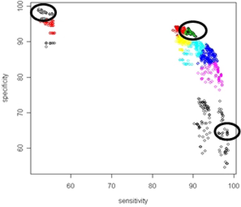
The CAIF simulator was setup to perform numerous iterations to produce a large variety of point assignment using randomized point assignment strategy where only unique combinations of points for each set were allowed. This produced a scatter plot of specificity against sensitivity, over which k-means clustering was applied to identify points that lie within the desired AOIs (Figure 12).

Figure 12.

Identified areas of interest

From Table 1, the three clusters of interest representing the AOIs were 2, 5 and 10 with the following centroids (98.35, 53.42), (66.50, 94.63) and (86.89, 94.41). For AOI(1), none of the point assignments provided a better result than simply running WMA algorithm which yielded (99.17, 52.12) as the specificity and sensitivity values. Thus, the conclusion was that the proposed framework does not provide any benefit in cases when highest possible specificity is desired. On the other hand, for AOI(2), the identified centroid of (66.50, 94.63) provided a cluster with about 125 point assignments some of which provided better results than any single algorithm.

Table 1.

Cluster centres

Cluster	Specificity (%)	Sensitivity (%)
1	92.94	88.15
2	98.35	53.42
3	84.93	92.50
4	90.15	87.38
5	66.50	94.63
6	88.28	90.78
7	94.52	54.74
8	89.10	54.39
9	81.46	95.92
10	86.89	94.41

For AOI(3), the identified centroid of (86.89, 94.41) is quite close to the result produced by EARS C3 algorithm. However, this cluster has over 200 point assignments some of which yield higher sensitivity and specificity values than EARS C3 which provides the best pair from all algorithms in the candidate set. For example, the following rule set yields (86.39, 95.50):

$$\langle 1_1^0{,2}_6^0{,3}_1^2{,4}_0^3{,5}_3^5{,6}_1^2\rangle$$

which translates to positive confidence associated with the following rules,

$$\left[\begin{array}{ll}{1}^R\hspace{0.17em}:\hspace{0.17em}NA\to 0\hspace{0.17em}points\hfill & \hfill \\ 2^R\hspace{0.17em}:\hspace{0.17em}NA\to 0\hspace{0.17em}points\hfill & \hfill \\ 3^R\hspace{0.17em}:\hspace{0.17em}{\phi }_{WMA}=true\to 2\hspace{0.17em}points\hfill & \hfill \\ 4^R\hspace{0.17em}:\hspace{0.17em}{\phi }_{C1}=true\to 3\hspace{0.17em}points\hfill & \hfill \\ 5^R\hspace{0.17em}:\hspace{0.17em}{\lambda }_d>T_u*{\lambda }_{d-1}\to 5\hspace{0.17em}points\hfill & \hfill \\ 6^R\hspace{0.17em}:\hspace{0.17em}{\omega }_d>T_d*{\omega }_{d-1}\to 2\hspace{0.17em}points\hfill & \hfill \\ \hfill & \hfill \end{array}\right]$$

Negative confidence points associated with the following rules,

$$\left[\begin{array}{ll}{1}_L\hspace{0.17em}:\hspace{0.17em}{\phi }_{CUSUM}=false\to 1\hspace{0.17em}point\hfill & \hfill \\ 2_L\hspace{0.17em}:\hspace{0.17em}{\phi }_{C3}=false\to 6\hspace{0.17em}points\hfill & \hfill \\ 3_L\hspace{0.17em}:\hspace{0.17em}{\phi }_{WMA}=false\to 1\hspace{0.17em}point\hfill & \hfill \\ 4_L\hspace{0.17em}:\hspace{0.17em}NA\to 0\hspace{0.17em}points\hfill & \hfill \\ 5_L\hspace{0.17em}:\hspace{0.17em}{\lambda }_d<T_u*{\lambda }_{d-1}\to 3\hspace{0.17em}points\hfill & \hfill \\ 6_L\hspace{0.17em}:\hspace{0.17em}{\omega }_d<T_d*{\omega }_{d-1}\to 1\hspace{0.17em}point\hfill & \hfill \\ \hfill & \hfill \end{array}\right]$$

Note that each side of the rule set contributes a maximum of M = 12 points providing an overall confidence measure ranging from −12 (100% negative confidence) to +12 (100% positive confidence).

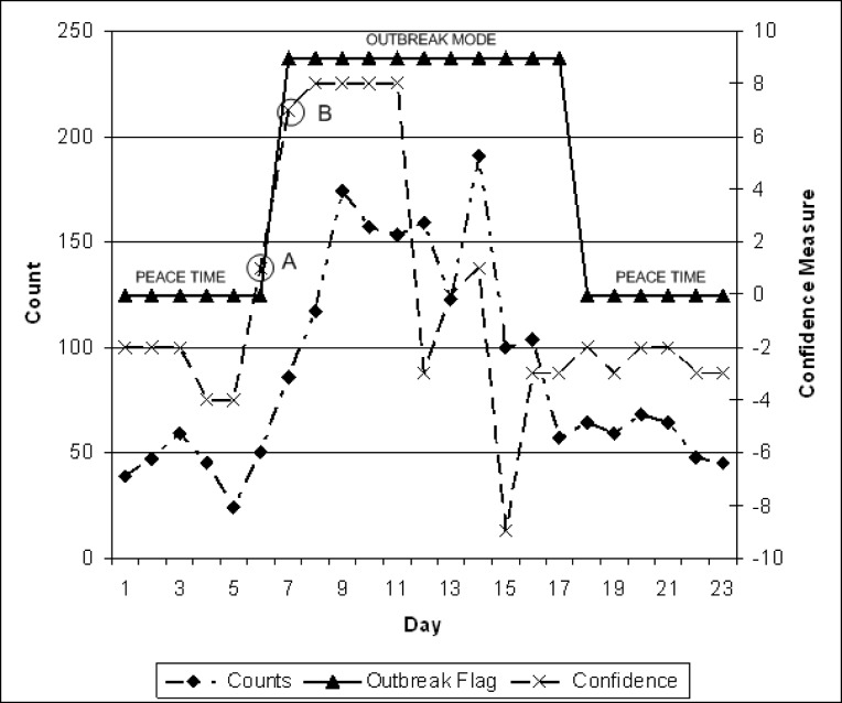
Next, one of the rule sets from the AOI(3) cluster were applied to a sample outbreak within the simulated data sets and confirm its effectiveness. (Figure 13) illustrates a snapshot that superimposes daily counts during outbreak mode along with computed confidence measure using the above rule set.

Figure 13.

Simulated outbreak analysis

As shown, the framework suggests an outbreak day with confidence measure of +1 ( $\frac{1}{12}$or 8.33% positive confidence) on day 6, a day before an outbreak is going to start (point A). Although a false positive decision, it is a weak false positive that aids in planning for the following day which will have a strong positive confidence measure of +7 translating to $\frac{7}{12}$ or 58.3% positive confidence (point B). This is exactly what the aim of this framework was set to be, that is, identify start of an outbreak with some level of confidence measure at an early stage. Further to note, as the outbreak progresses, the confidence seems to drop to negative values. This is because the framework is intended to monitor initial start of an outbreak. As the values stabilize during an outbreak, the confidence measure of start of an outbreak will diminish as expected.

A detailed step by step simulation results for the proposed framework have been provided in [10].

6. Real scenario

The rule set for AOI (3) from previous section was applied to a subset of real emergency room visit data from the Canadian Early Warning System (CEWS).

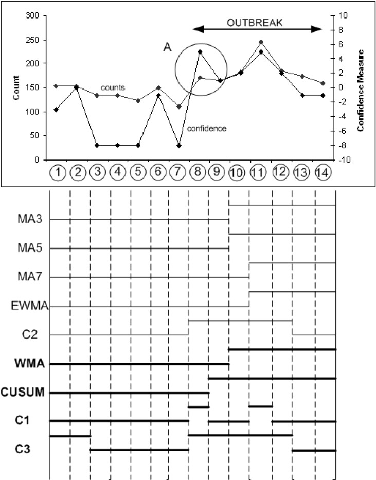
As shown in Figure 14, one of the key observations is that the indication that an outbreak is going to occur in the next few days was identified by a higher confidence value on Day 8, which was most likely the first day of an outbreak curve with peak on Day 11. Further, the confidence measure was computed based on a minimal set identified by the proposed framework and not the entire set of nine algorithms. That is, the minimal set identified by the proposed framework was sufficient to detect the start of an event a few days earlier than it was actually detected.

FIGURE 14.

Application of CIAF to Real Scenario

The following is some analysis of some of the days with interesting observations.

• Day 8: Three of nine algorithms suggest an outbreak out of which two are from the identified minimal set. Looking at this at face value would produce a biased decision that we had no signs of start of an outbreak on day 8. However, considering only the minimal set, there is a split decision, and using the proposed point assignment system a confidence measure of +5 translating to 5/12 or 41.7% positive confidence is produced. Thus, there were clear signs for start of an outbreak on that day as suggested by a strong confidence value.

• Day 9: The confidence value drops drastically to just above the 0 or no decision line. This is due to the actual count staying at similar level as the count for previous day thus the λ and ω values did not change much and did not contribute to the overall confidence value as strongly as they did on the previous day. However, the confidence value still stayed above zero point indicating some level of activity.

• Day 11: This is the day when the counts of cases during an outbreak are the highest. All four algorithms of the minimal set declare an outbreak, however, the framework produces confidence measure of only +5. This is because the framework is monitoring start of an outbreak and not necessarily the peak. At the peak, both λ and ω do not contribute their portion to the overall confidence measure since neither the recent most count nor the count delta satisfy the rules as defined in the positive set.

Using the proposed framework, the identification with significant confidence would have been detected on Day 8 and initial start of some activity instead of delayed identification which most likely occurred on Day 11.

7. Limitations

The following list highlights some limitations of the proposed framework and thus potential areas for future research:

1. Identification of Optimal Rule: The proposed framework employs basic techniques for clustering and point identification. Use of more sophisticated clustering techniques as well as optimal point identification systems to come up with best rule to use within a given area of interest.

2. Further Generalization: It would be useful to implement of other versions of exponential smoothing schemes which include seasonality corrected approach and apply to the overall framework.

3. Time Effect: Taking into account time of day, day of week, week of month and month of year within the framework and use it to deduce further redundancy between various algorithms.

4. Data Labeling: A feedback mechanism for public health specialists to close the loop for labeling outbreaks and no-outbreak decisions. This will extend the framework to allow for other techniques for evaluation purposes.

5. Invariant Minimal Set: There is no question that some algorithms are better than others when looking at different disease outbreaks. Applying a variety of outbreak types to the data (beyond log normal, daily spikes, etc) will help in figuring out if the minimal set produced by the framework is invariant.

8. Conclusion

A novel aberration interpretation framework has been proposed for producing a confidence based system decision focusing on high confidence values at the start of an outbreak. The framework comprises of multiple steps to allow identification of a subset of algorithms as well as a dynamic point assignment scheme for computing a balanced decision.

The proposed framework provides a multitude of benefits:

• Savings in the computation effort by identifying only a smaller subset of algorithms that are necessary and sufficient for a sound system decision.

• Provides a mechanism to derive confidence value based on dynamic point assignment system.

• Produces a superior overall system decision within desired AOI when compared to any single algorithm.

• Provides a framework for future research to investigate optimal point allocation systems as well as analysis of new algorithms and their effects on the overall decision.

The proposed framework is also adaptable or extensible. It captures the essential elements of a confidence based decision process.

References

- 1.Jackson M, Baer A, Painter I, Duchin J. A simulation study comparing aberration detection algorithms for syndromic surveillance. BMC Medical Informatics and Decision Making. 2007;7 doi: 10.1186/1472-6947-7-6. [DOI] [PMC free article] [PubMed] [Google Scholar]
- 2.Centre for Disease Control (CDC) Data Sets. Available at: http://www.bt.cdc.gov/surveillance/ears/datasets.asp.
- 3.Trochim W. Correlation. Available at: http://www.socialresearchmethods.net/kb/statcorr.htm.
- 4.Jacob C. A coefficient of agreement for nominal scales. Educational and Psychological Measurement. 1960;20:37–46. [Google Scholar]
- 5.Landis J, Koch G. The measurement of observer agreement for categorical data. Biometrics. 1977;33(1):159–174. [PubMed] [Google Scholar]
- 6.Waner S, Costenoble S. Linear Regression. Available at: http://people.hofstra.edu/faculty/stefan_waner/realworld/tutorialsf0/frames1_5.html.
- 7.Wikipedia K-Means Algorithm. Available at: http://en.wikipedia.org/wiki/K-means_algorithm.
- 8.The R Package for Statistical Computing. Available at: http://www.r-project.org/
- 9.Hutwagner L, Thompson W, Seeman G, Treadwell T. The Bioterrorism Preparedness and Response Early Aberration Reporting System (EARS) Journal of Urban Health: Bulletin of the New York Academy of Medicine. 2003;80(2, Supplement 1):i89–i96. doi: 10.1007/PL00022319. [DOI] [PMC free article] [PubMed] [Google Scholar]
- 10.Mukhi S. PhD Thesis. University of Manitoba; Jun, 2007. An Integrated approach to Real-Time Biosurveillance in a Federated Data Source Environment. [Google Scholar]