Statistical shape analysis of the corpus callosum in Schizophrenia

Abstract

We present a statistical shape-analysis framework for characterizing and comparing morphological variation of the corpus callosum. The midsagittal boundary of the corpus callosum is represented by a closed curve and analyzed using an invariant shape representation. The shape space of callosal curves is endowed with a Riemannian metric. Shape distances are given by the length of shortest paths (geodesics) that are invariant to shape-confounding transformations. The statistical framework enables computation of shape averages and covariances on the shape space in an intrinsic manner (unique to the shape space). The statistical framework makes use of the tangent principal component approach to achieve dimension reduction on the space of corpus callosum shapes. The advantages of this approach are – it is fully automatic, invariant, and avoids the use of landmarks to define shapes.

We applied our method to determine the effects of sex, age, schizophrenia and schizophrenia-related genetic liability on callosal shape in a large sample of patients and controls and their first-degree relatives (N=218). Results showed significant age, sex, and schizophrenia effects on both global and local callosal shape structure.

Introduction

The corpus callosum is the largest inter-hemispheric commissural pathway in the brain. It is composed of an aggregated bundle of neural fibers of varying thicknesses that clusters to form a mass at the midline and extends to topographically homologous regions in each hemisphere. The corpus callosum has been widely investigated for its role in hemispheric communication and in lateralized brain function and behaviors. Callosal morphology varies with individual differences such as age, sex and intellectual ability (Luders et al., 2010, 2011). Several neurodevelopmental disorders also directly or indirectly affect the structural integrity and connectivity of the corpus callosum. For example, variations in callosal size and shape are associated with disease processes in autism and schizophrenia (Frazier and Hardan, 2009; Innocenti et al., 2003; Narr et al., 2000; Paul et al., 2007). In schizophrenia, the structural integrity and shape of the callosum reflect a genetic predisposition for the illness (Knöchel et al., in press; Narr et al., 2000, 2002). Bookstein et al. (2002b, 2007) and Downhill et al. (2000) have shown abnormalities in callosal anatomy due to neuro-toxicological insults to the fetus caused by prenatal alcohol exposure, resulting in fetal alcohol syndrome (FAS). In addition to the structural abnormalities linked with many neurological and psychiatric conditions, certain genetic disorders give rise to complete or partial agenesis (lack of development) (Paul et al., 2007) of the corpus callosum in early development. There are additional callosal malformations classified as dysgenesis (abnormal development) (Kendall, 1983), hypogenesis (partial development) (Van Bon et al., 2008) and hypoplasia (under-development) (Bodensteiner et al., 1994). Although the callosal fibers project widely into each cerebral hemisphere, the callosal midsagittal boundary of the cross-section is most widely studied (e.g., Downhill et al., 2000; Dutt et al., 2011; John et al., 2008; Luders et al., 2007, 2009; Narr et al., 2000; Rotarska-Jagiela et al., 2008; Walterfang et al., 2008; Weber et al., 2007; Witelson, 1989), both because there are reported relationships between fiber number and callosal area (Aboitiz et al., 1992; Riise and Pakkenberg, 2011) and due to the convenience in identification, representation, and analysis. This two-dimensional representation reduces the anatomical complexity resulting from the divergent extensions of the fiber branches to an efficient planar form, leading to straightforward and highly reproducible measurements of important structural properties such as the width, thickness, and area. In this paper we focus on the geometry of the midsagittal callosal boundary, propose a method for representing the shape of the corpus callosum, and also provide a statistical framework for performing morphometric analysis. Specifically, these methods were applied to confirm and extend prior findings concerning effects of sex and age and callosal shape abnormalities in schizophrenia and disease-related genetic liability.

Background

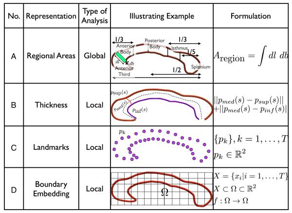
Over the past decade, several researchers have proposed different methods for representation and analysis of the cross-sectional boundary of the corpus callosum. We summarize some of the prominent boundary-based approaches in this section. Fig. 1 illustrates these approaches. An early morphometric approach by Witelson subdivides the corpus callosum into seven regions to examine parcellated midsagittal areas (Witelson, 1989). A similar approach (Clarke and Zaidel, 1994; Hofer and Frahm, 2006) also obtains a regional parcellation of the corpus callosum based on the topographical structure of the fibers with respect to their connections with cortical regions. For example, Fig. 1(A) shows a typical regional subdivision scheme (Clarke and Zaidel, 1994; Rajapakse et al., 1996; Witelson, 1989) that divides the callosal boundary into the splenium (temporal, inferior, and occipital nerve fibers), the isthmus (superior temporal, posterior parietal), the posterior midbody (posterior, parietal), the anterior body (motor), and the anterior third (prefrontal fibers). Another approach (Fig. 1(B)) measures the width or the thickness of the callosal boundary by calculating the distance to the medial line of the superior and the inferior boundaries (Luders et al., 2010; Thompson et al., 2003). A follow-up to this approach (Adamson et al., 2011) solves the Laplace equation between the superior and inferior boundaries and computes streamlines to measure thickness. Alternately one can discretize the callosal shape by identifying point landmarks on the boundary, and normalize the landmarks by centering and scaling them appropriately (Fig. 1(C)). This allows one to conduct the shape analysis by performing a Procrustes-based alignment of the landmarks (Bookstein et al., 2002a) and computing mean landmark shapes, or by embedding the landmarks in a two-dimensional planar region (Fig. 1(D)), and warping the whole region using methods such as thin plate splines (Bookstein et al., 2002a) or diffeomorphic non-rigid registration (Guo et al., 2004). In addition, there are other approaches (El-Baz et al., 2011) that represent the corpus callosum using a three-dimensional surface representation instead of a two-dimensional boundary.

Fig. 1.

Different approaches for boundary analysis of the corpus callosum.

Approach

Here, we represent the mid-sagittal boundary of the corpus callosum by a closed curve and analyze its shape, by imposing appropriate geometric invariances including rigid motions and scaling on the curve. We also provide a framework for dimension reduction of the population shape variables through principal component analysis (PCA) in the tangent space of the mean shape. This not only allows local geometric shape analysis via tangent vectors to the geodesics to characterize infinitesimal changes along the boundary, but also highlights global changes in shape covariates using the dominant modes of population variation. The key advantage of this approach is that it permits the use of callosal shape as a geometric phenotype in more sophisticated multivariate analyses investigating the influence of sexual dimorphism, development, and disease on the structure of the corpus callosum.

We suggest that there is a difference between methods that perform registration as a prelude to shape analysis, and those that perform intrinsic statistical shape analysis. The goal of registration methods is to establish correspondences (one-to-one) between pairs of shapes, usually in an ambient Euclidean space after factoring out affine/rigid/non-rigid motions and/or uniform scaling. The resulting statistical analysis is then carried out in the ambient space where the template is either selected as a predetermined observation from the population, or constructed using Euclidean averages. The aim of an intrinsic shape analysis framework is to additionally achieve accurate registration and correspondences between shapes and to focus on the representation of the shape and the underlying shape space, thereby allowing the computation of all the statistical estimates native to the space. Thus the objectives of such an intrinsic statistical shape analysis framework encompass correspondence-based registration methods while simultaneously integrating the tools for statistical analysis into a nonlinear registration framework.

Our approach is fundamentally different from previously proposed approaches that represent shapes as parametric contours using b-spline snakes (Brigger et al., 2000) or active contour models for which a) the underlying representation is finite-dimensional (b-spline coefficients, or landmarks for active contours), b) the primary focus is on registration or segmentation, c) intrinsic statistical shape analysis is not possible. Thus to our knowledge, this is the first approach where the corpus callosum is represented by an invariant parameterized curve and directly analyzed by the shape of its boundary. Here, we outline a comprehensive computational framework for corpus callosum shape as applied to the study of a large number of subjects (N=218) including patients with schizophrenia, unaffected relatives of patients and community comparison subjects. This framework provides i) nonlinear elastic matching between callosal shapes for accurate local shape correspondences, ii) a full path of deformations between callosal shapes that highlights local shape differences, iii) an efficient computation of geodesics in the shape space of corpus callosum curves, iv) a tangent vector that not only encodes the shape changes between curves, but also helps to locally linearize the shape space, and most importantly v) tools for computing shape means and covariances that enable a full statistical analysis of the morphology of the corpus callosum that may associate it with individual differences such as sex, age and disease state.

This paper is organized as follows. The callosal shape representation, the pre-shape space, and the metric on the tangent space are described in the Corpus callosum shape representation section. The methods for shape matching, representing invariances, and computing the geodesics by factoring out nuisance variables are described in the Invariance to nuisance variables and Corpus callosum shape matching sections. The intrinsic statistical shape analysis framework is discussed in the Karcher mean section that outlines the procedure for the computation of the Karcher mean, performing the tangent principal component analysis (TPCA) at the mean shape, and for reconstructing and synthesizing the shapes from the TPCA model. In the Results section we will present the application of this to a sample of 218 shapes to examine the effects of sex, age, schizophrenia and schizophrenia-related genetic predisposition.

Methods

This section describes the curve-based boundary representation for the corpus callosum as an element in a shape space, endowed with a differentiable geometric metric. Quantitative differences between different boundaries are obtained by computing shortest paths or geodesics between them on the shape space. These geodesics also provide a smooth minimal energy deformation path from one boundary to another. The advantage of these paths are twofold, i) the length of the path yields a single scalar value quantifying the difference between two shapes, and ii) the gradual local changes of deformations along the path provides a visual representation of the structural differences between the shapes. Additionally geodesics are also useful in the construction of manifold averages for populations of shapes, an important requirement in statistical analysis of shapes.

Corpus callosum shape representation

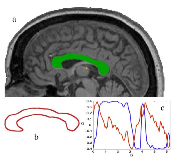
We represented the two-dimensional boundary of the corpus callosum by a contour corresponding to four mid-sagittal planar boundary in the brain MRI image. To reduce noise we averaged the contour tracings of the para-sagittal boundaries and used the average contour as the callosal boundary. Fig. 2(a) shows a mid-sagittal slice of an MRI image with the corpus callosum shown as a green mask. The boundary of the callosal region is extracted and shown as a curve (Fig. 2(b)). Mathematically the corpus callosum curve is parameterized (Joshi et al., 2007a, 2007b; Srivastava et al., 2011) by a closed continuous curve β, such that $\beta :[0,2\pi ]\to {\mathbb{R}}^2$, and its shape is defined by the function $q:[0,2\pi ]\to {\mathbb{R}}^2$ as

$$q\left(s\right)=\frac{\stackrel{.}{\beta }\left(s\right)}{\sqrt{\Vert \stackrel{.}{\beta }\left(s\right)\Vert {\mathbb{R}}^2}}\in {\mathbb{R}}^2.$$ (1)

Fig. 2.

a) Mid-sagittal slice of a T1 MRI image with the corpus callosum region highlighted in green, (b) a two-dimensional manual tracing of the boundary of the corpus callosum, and (c) two components of the vector valued function q over the boundary.

This vector valued function measures the tangent vector normalized by the square-root of the instantaneous speed along the curve and is a local descriptor of the geometry of the curve. The quantity s,s∈[0,2π] is the parameterization of the curve, and is a function itself. The instantaneous velocity of the curve is given by the derivative $\stackrel{.}{\beta }\left(s\right)$. As an example, Fig. 2(c) shows the plot of the function q for the curve β in Fig. 2(b). The original curve β can be reconstructed up to a translation using $\beta \left(s\right)={\int }_0^s\Vert q\left(t\right)\Vert q\left(t\right)dt$. Throughout this paper we denote the callosal curve as a coordinate function given by the curve β, and the callosal shape given by the vector valued function q. Since we are exclusively interested in modeling the geometric shape of the corpus callosum, we factor out the size or scale from the representation by normalizing the function q. The scale invariant shape representation is given by normalizing the function q by its magnitude as $\frac{q}{\sqrt{{\int }_0^{2\pi }{\left(q\right(s),q(s\left)\right)}_{{\mathbb{R}}^2}ds}}$. The norm in the denominator is a Euclidean norm, and ${(.,.)}_{{\mathbb{R}}^2}$ is the standard Euclidean inner-product in ${\mathbb{R}}^2$. Throughout this paper, the function q refers to this scale-invariant form unless indicated otherwise. Due to this unit-scaling constraint, the space of all translation and scale-invariant shapes becomes a Hilbert sphere denoted by $\mathcal{Q}$. Formally, the space $\mathcal{Q}$ is defined as

$$Q\equiv \left\{q\in {\mathbb{L}}^2\left({\mathbb{R}}^2\right)\mid {\int }_0^{2\pi }{\left(q\right(s),q(s\left)\right)}_{{\mathbb{R}}^2}ds=1,q\left(s\right):{\mathbb{S}}^1\leftarrow {\mathbb{R}}^2\phantom{\mid }\right\}.$$ (2)

To represent closed boundaries, we impose an additional closure constraint on the callosal curves. This closure constraint is written as ${\int }_0^{2\pi }\stackrel{.}{\beta }\left(s\right)ds=0$, in terms of the coordinate function, and is speci fied as ${\int }_0^{2\pi }q\left(s\right)\Vert q\left(s\right)\Vert ds$ in terms of the callosal shape function. We then define the set of such translation, scale-invariant, and closed representations as the pre-shape space of the corpus callosum shapes and denote it by

$$\mathcal{C}\equiv \left\{q\mid q\in Q,{\int }_0^{2\pi }q\left(s\right)\Vert q\left(s\right)\Vert ds=0\right\}.$$ (3)

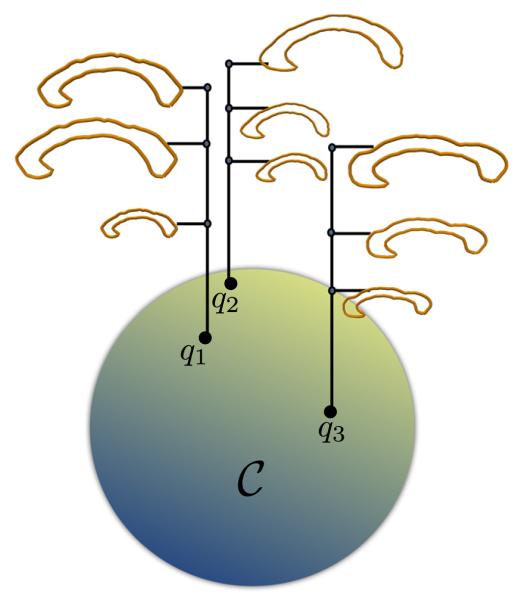
This pre-shape space $\mathcal{C}$ is actually a subset of an in finite-dimensional unit-sphere as a result of the scale-invariant constraint and represents all closed elastic curves invariant to translation and uniform scaling. Fig. 3 shows a schematic of the callosal boundary representation on the pre-shape space. Each corpus callosum curve with varying size, but having the same shape is projected as a single element of the pre-shape space $\mathcal{C}$. An important geometrical construct for the statistical analysis of the callosal shapes is the definition of a tangent space. The tangent space allows for local linearization of the shape space and enables the use of Euclidean shape statistics for a population. The tangent space of $\mathcal{C}$ is de fined by the collection of all tangent vectors perpendicular to the normal space of$\mathcal{C}$. The span of the gradient vector field of the closure constraint of q defines the normal space of all closed curves. The closure constraint on the curves is ${\int }_0^{2\pi }\left[\begin{array}{c}\hfill q^1\left(s\right)\hfill \\ \hfill q^2\left(s\right)\hfill \end{array}\right]\Vert q\left(s\right)\Vert ds=0$, where q¹(s), and q²(s) are the two components of q. Then the normal space of all closed curves at q given by the span of the directional derivative of the closure condition as

$$N_q\left(\mathcal{C}\right)=\text{span}\left\{\frac{q^1\left(s\right)}{\Vert q\left(s\right)\Vert }q\left(s\right)+\Vert q\left(s\right)\Vert \left[\begin{array}{c}\hfill 1\hfill \\ \hfill 0\hfill \end{array}\right],\frac{q^2\left(s\right)}{\Vert q\left(s\right)\Vert }q\left(s\right)+\Vert q\left(s\right)\Vert \left[\begin{array}{c}\hfill 0\hfill \\ \hfill 1\hfill \end{array}\right]\right\}.$$ (4)

Fig. 3.

Schematic of the pre shape space of scale and translation invariant curves.

The tangent space of $\mathcal{C}$ at q, denoted by $T_q\left(\mathcal{C}\right)$ is given by

$$T_q\left(\mathcal{C}\right)\equiv \left\{v\mid v\perp Q,v\perp N_q\left(\mathcal{C}\right)\right\}.$$ (5)

As described in (Joshi et al., 2007a, 2007b), we equip the tangent space of $\mathcal{C}$ with a smoothly varying metric that measures in finitesimal lengths on the pre-shape space. This inner product is first defined generally on the space of all q functions and then induced on the tangent space of $\mathcal{C}$. Given a pair of tangent vectors $u,v\in T_q\left(\mathcal{C}\right)$ the metric is defined as,

$$\langle u,v\rangle ={\int }_0^{2\pi }\left(u\right(s),v(s\left)\right){{}_{\mathbb{R}}}^{2}ds.$$ (6)

Invariance to nuisance variables

The main ingredients for matching the anatomy of the corpus callosum on the shape space are i) identification of geometrical confounds or nuisance variables that do not affect the shape, ii) modeling the nuisance variables using suitable mathematical structures, and finally iii) constructing geodesics or shortest-distance paths on the shape space by factoring out the nuisance variables. Since the corpus callosum is a closed curve, the starting point or origin on the curve is arbitrary. Thus irrespective of whether the boundary of the shape is manually traced or automatically detected, the shapes for different subjects are not assumed to have their arbitrary origins or starting points registered. Likewise the corpus callosum boundaries may not always be consistently oriented across subjects. Lastly, callosal curves can be parameterized by non-uniform speeds without changing their shape. This non-uniformity usually arises from the tracing or the extraction protocol used. Moreover all of the above nuisance variables are also affected by volumetric registrations that may be applied at various preprocessing stages to normalize the original MRI images. An important point to note here is that the geometric shape is not affected by the registration results so long as they are rigid-body (6-parameter) registrations with or without the addition of uniform scaling. Importantly, while performing the actual shape matching, rather than fixing the values of these nuisance variables or obtaining a canonical representation for them in advance, we treat the nuisance variables as elements of equivalence classes under the respective transformations. This is achieved as follows. Translation and scaling are automatically removed due to the shape representation by the q function. A rigid rotation of a curve is a shape-preserving operation, also considered as a group action by a 2×2 rotation matrix O∈SO(2) applied to q, and is defined as O·q(s)=Oq(s), ∀s∈[0,2π]. A change in the starting point of the curve $q\in \mathcal{C}$ is represented by the action of a unit circle S¹ on q, according to r·q(s)=q((s–r)_{mod 2π}) for r∈[0,2π]. This action due to the placement of the origin simply shifts the shape by the quantity r. Lastly, the reparameterization of a curve that traveled at arbitrary speeds is represented by a non-linear differentiable map γ (with a differentiable inverse) also referred to as a diffeomorphism. We define $\mathcal{D}=\{\gamma :{\mathbb{S}}^1\to {\mathbb{S}}^1\}$ as the space of all orientation-preserving diffeomorphisms. Then the resulting variable speed parameterizations of the curve can be thought of as diffeomorphic group actions of $\gamma \in \mathcal{D}$ on the curve and given as $q\cdot \gamma =\sqrt{\stackrel{.}{\gamma }}(q°\gamma )$. Table 1 lists the nuisance variables that affect the pose, translation, orientation, and reparameterization of the callosal curve while leaving its shape unchanged.

Table 1.

Geometrical confounds for corpus callosum shape analysis

Shape confound	Source	Symbol	Space
Translation	Head position/scanner	T	${\mathbb{R}}^3$
Scaling	Head volume/scanner	a	${\mathbb{R}}_{+}$
Rotation	Head position/scanner	$O\in {\mathbb{R}}^{2\times 2}$	SO(2)
Starting point/origin	Tracing/extraction	r∈[0,2π)	${\mathbb{S}}^1$
Reparameterization	Representation/tracing/extraction	γ∈[0,2π)	$\mathcal{D}$

Ultimately, we are interested in analyzing callosal shapes in the invariant space of shapes given by the quotient space of $\mathcal{C}$ modulo shape preserving transformations including change in origins, rigid rotations and reparameterizations. Consequently, the provision of the reparameterization operation facilitates elastic shape analysis of callosal curves. Thus the elastic shape space is defined as the quotient space

$$S=C∕\left({\mathbb{S}}^1\times \mathrm{SO}\left(2\right)\times \mathcal{D}\right).$$ (7)

Corpus callosum shape matching

In this section, we describe the shape matching procedure between corpus callosum boundaries. Specifically we outline a procedure for computing geodesics between a pair of corpus callosum shapes under the Riemannian metric defined in the Corpus callosum shape representation section. For a better understanding, we describe the procedure for computing geodesics in the ambient space $\mathcal{Q}$ and the pre-shape space $\mathcal{C}$ of all closed callosal curves first.

Shape matching in the space of q functions of callosal boundaries

As noted earlier, the space of scale-invariant q functions of callosal boundaries is a Hilbert sphere. Thus the translation and scale-invariant geodesic distance between a pair of callosal shapes q₁ and q₂ in the space $\mathcal{Q}$ is given by

$${\chi }_t(q_1;f)=\mathit{cos}\left(t{\mathit{cos}}^{-1}\langle q_1,q_2\rangle \right)q_1+\mathit{sin}\left(t{\mathit{cos}}^{-1}\langle q_1,q_2\rangle \right)f,$$ (8)

where the initial tangent vector $f\in T_{q_1}\left({\mathbb{S}}^q\right)$ is given by f=q₂–⟨q₁,q₂⟩ q₁. Eq. 8 is the analytical solution of a geodesic on the sphere. The tangent space projection of the vector f at q₁ is obtained as $f=\frac{\theta \cdot f}{\sqrt{\langle f,f\rangle }}$, where θ=arccos{⟨q₁,q₂⟩}. The successive shapes along the geodesic are obtained by taking incremental steps in the direction of f for short time intervals dt, while projecting the tangent vector f on the tangent space at the subsequent shape. Then the geodesic distance between the two shapes q₁ and q₂ in $\mathcal{Q}$ is given by

$$d(q_1,q_2)={\int }_0^1\sqrt{\langle {\stackrel{.}{\chi }}_t,{\stackrel{.}{\chi }}_t\rangle }dt.$$ (9)

The quantity χ_t is also referred to as the velocity vector along the geodesic path χ_t. It is also noted that χ₀(q₁)=q₁, and χ₁(q₁)=q₂.

Shape matching in the pre-shape space C of closed callosal boundaries

Since the pre-shape space $\mathcal{C}$ consists of shapes of closed callosal curves, the geodesics are constructed by first initializing a path between q₁ and q₂ in the space of open curves $\mathcal{Q}$, and then successively modifying it to form a geodesic in $\mathcal{C}$.

We denote an arbitrary path between two shapes in $\mathcal{C}$ by ${\alpha }_t:t\in [0,1]\to \mathcal{C}\mid {\alpha }_0=q_1,{\alpha }_1=q_1$, such that the velocity vector along the path is given by ${\stackrel{.}{\alpha }}_t,t\in [0,1]$. Then α is a geodesic if it minimizes the energy $E=\frac{1}{2}{\int }_0^1\langle {\stackrel{.}{\alpha }}_t,{\stackrel{.}{\alpha }}_t\rangle dt$. We use a path-straightening flow that employs gradient descent to iteratively minimize the energy E and find the geodesic in $\mathcal{C}$. Then the geodesic distance between the shapes q₁, and q₂ in the pre-shape space $\mathcal{C}$ is given as

$$d_c(q_1,q_2)={\int }_0^1\sqrt{\langle {\stackrel{.}{\alpha }}_t,{\stackrel{.}{\alpha }}_t\rangle }dt.$$ (10)

It is important to note that a geodesic in $\mathcal{C}$ may be longer than a geodesic in $\mathcal{Q}$ since $\mathcal{C}$ excludes those regions of $\mathcal{Q}$ corresponding to non-closed curves.

Shape matching in the space $\mathcal{S}$ of invariant callosal shapes

To obtain fully invariant shape matching with regard to the nuisance variables listed in Table 1, correspondence between a pair of shapes is calculated using a geodesic between the respective equivalence classes on the shape space $\mathcal{S}$. This is achieved by first constructing a geodesic in the pre-shape space $\mathcal{C}$, and then optimizing over the placement of origin, the rotation, and the reparameterization of the shape. This is realized by first finding a geodesic in the quotient space $\mathcal{C}∕\left({\mathbb{S}}^1\times \mathrm{SO}\left(2\right)\right)$, and then optimizing over origin placement, rotation and reparameterization group in the quotient space $\mathcal{C}∕\left({\mathbb{S}}^1\times \mathrm{SO}\left(2\right)\right)∕\mathcal{D}$, described briefly as follows. The optimal placement of origin is given by

$$\widehat{r}=\underset{r}{\mathrm{arginf}}{\int }_0^{2\pi }{\langle q_1-r^{.}{q}_2,q_1-r^{.}{q}_2\rangle }^2,$$ (11)

and in practice found by keeping q₁ fixed, and exhaustively searching over all points of the shape q₂. The optimal rotation $\left(\widehat{O}\right)$ is found by carrying out a singular value decomposition (Rohlf and Slice, 1990)

$$\widehat{O}={\mathit{ADB}}^T={\int }_0^{2\pi }{q}_1\left(s\right)q_2{\left(s\right)}^{T}ds,$$ (12)

where A and B are left and right unitary matrices, and D is a matrix given by

$$D=\left[\begin{array}{cc}\hfill 1\hfill & \hfill 0\hfill \\ \hfill 0\hfill & \hfill \mid A\mid \mid B\mid \hfill \end{array}\right].$$ (13)

Lastly the optimal reparameterization $\widehat{\gamma }$ is found as the minimizer

$$\widehat{\gamma }=\underset{\gamma }{\mathrm{argmin}}\left({\int }_0^{2\pi }\left[{\Vert q_1-{\gamma }^{.}{\tilde{q}}_2\Vert }^2+{\Vert {\tilde{q}}_2-{\gamma }^{-1.}{q}_1\Vert }^2\right]ds\right),$$ (14)

where ${\tilde{q}}_2=\widehat{r}\cdot \widehat{O}{q}_2$. Eq. 14 is solved using dynamic programming. After the optimal geodesic is found by optimizing over the nuisance variables, the distance between two shapes is given by

$$d_S(q_1,q_2)=d_C\left(q_1,\left({\widehat{r}}^{.}\widehat{O}{q}_2\right)\cdot \widehat{\gamma }\right),$$ (15)

where d_C is given by Eq. 10. The optimal geodesic path can also be denoted by a one-parameter flow Ψ and the tangent vector ${\stackrel{.}{\alpha }}_t$, such that

$${\Psi }_t:t\in [0,1]\to S\mid {\Psi }_0(q_1,{\stackrel{.}{\alpha }}_t)=q_1,{\Psi }_1(q_1,{\stackrel{.}{\alpha }}_t)=\left(\widehat{r}\cdot \widehat{O}{q}_2\right)\cdot \widehat{\gamma }\phantom{\mid }.$$ (16)

Alternatively, the optimal tangent vector can be written from Eq. 16 as

$${\stackrel{.}{\alpha }}_t-{\psi }_1^{-1}\left(q_1,\left(\widehat{r}\cdot \widehat{O}{q}_2\right)\cdot \widehat{\gamma }\right).$$ (17)

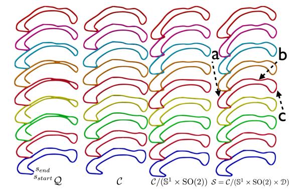
We note that the procedure for finding geodesics between two corpus callosum shapes not only provides the optimal elastic correspondence between them, but also provides an intrinsic framework for statistical shape analysis by locally capturing the non-linearity of the shape space. As an example, Fig. 4 shows geodesic paths (top to bottom) between two shapes in different spaces. To illustrate the effect of different constraints on shapes, we purposefully select two shapes that have a small opening at the genu where the operator performing manual tracing chose end points for the closed curves that were somewhat distant from the starting points. The first column of Fig. 4 shows the path in the space $\mathcal{Q}$ of all q functions. We observe that the intermediate shapes along the geodesic cause the gap to widen reflecting the absence of a closed curve constraint in $\mathcal{Q}$ and also result in an abnormal reduction in the thickness of the corpus callosum. The second column shows the geodesic in $\mathcal{C}$. Due to the closure constraint, the intermediate shapes are now closed, and there is no compression of thickness. The third column shows a geodesic after optimizing over origin placement and rotation, whereas the last column shows the fully invariant geodesic. Comparing the last two columns, we note that the optimization over the reparameterization makes a noticeable difference in the intermediate shapes along the path. Due to the elastic matching, important features such as the shape of the genu (label a), the contraction in the mid-posterior section (label b), and the bulbous region (label c) of the splenium are preserved along the path. Fig. 5 shows selected correspondences between the top and bottom shapes in Fig. 4 with lines drawn between corresponding points of the two shapes matched in spaces C/(S¹×SO(2)) and S. We observe that the elastic matching in S yields a better homological correspondence compared to the non-elastic matching. For example, neither the tip of the genu, nor the posterior region is correctly matched in the non-elastic case, whereas in the elastic case, salient features in both the shapes are in correspondence due to the optimal non-linear matching. Fig. 5(C) shows the non-linear correspondence function $\widehat{\gamma }$ between the two shapes compared with the linear case (γ=s).

Fig. 4.

Geodesic paths (top to bottom) between two shapes in different pre-shape spaces, and the shape space S. The labeled arrows point to regions where noticeable changes in the shape along the path in S compared to the path in $\mathcal{C}∕\left({\mathbb{S}}^1\times \mathrm{SO}\left(2\right)\right)$ are observed. In the column $\mathcal{Q}$, s_tart, and s_end are the end-points of the shape respectively.

Fig. 5.

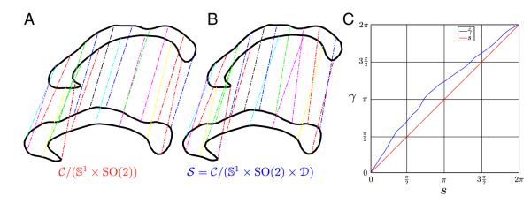
Correspondence between shapes using non-elastic matching (A), and elastic matching (B). The optimal elastic ($\widehat{\gamma }$) correspondence function is overlaid on the linear (γ=s) matching function (C).

Using this optimal matching, our primary objective is to model the underlying statistical shape variability of the corpus callosum in a given population as detailed in the next section.

Statistical shape analysis

Since the shape space is non-linear and infinite dimensional, conventional multivariate statistical methods cannot be applied in a straightforward manner. A computational framework that adapts the statistical tools to our shape space is thus required. The statistical shape average is computed as a first step towards this goal. The tangent vectors corresponding to geodesics from the average shape to each individual shape encode the first order linear variations of the shapes in the population about the mean shape. This means that the original shape is recoverable by constructing a one-parameter flow along its tangent vector from the mean. Therefore the collection of tangent vectors along the geodesics for the entire population represent a locally linearized version of the shape space at the mean shape and form a population-based linear basis of the shape observations in the dataset. The tangent-space representation circumvents the need to explicitly model the non-linearity of the shape space. Finally, to overcome the difficulty in modeling the conceptually infinite dimensionality of the tangent vectors and hence of the tangent space, dimensional reduction in the tangent space is performed using principal component analysis (PCA). This computational technique, also known as tangent PCA (TPCA), has also been previously used for dimension reduction on non-linear manifolds in different settings (Fletcher and Joshi, 2004; Vaillant et al., 2004). In the following sections, we outline the framework for performing statistical shape analysis for corpus callosum shapes.

Karcher mean

We use the notion of the intrinsic mean (Bhattacharya and Patrangenaru, 2002; Le, 2001; Woods, 2003) for computing shape averages on the manifold. Numerous advantages of the intrinsic approach over the more conventional extrinsic approach are detailed in the literature (Fletcher and Joshi, 2004; Vaillant et al., 2004), and we only outline the main differences briefly. The extrinsic approach relies on a Euclidean embedding of the shapes in the ambient space and projects the Euclidean average on the shape space. It is very simple and efficient to compute, but it does not account for the nonlinear nature of the shape space. Specifically the extrinsic average ignores the underlying Riemannian metric and does not achieve optimal matching between shapes. On the other hand, the intrinsic approach builds upon the local metric and relies exclusively on the distances defined on the shape space. This approach is invariant to rotations, translations, scaling, and reparameterizations and is thus a preferred choice for computing statistical estimates on shapes. The intrinsic mean is also known as the Karcher mean (Le, 1995; Srivastava et al., 2005) and is defined for a set of shapes {q_i},i=1,…,N as

$$\mu =\underset{q_{\mu }}{\mathit{arg}\mathit{min}}\sum _{i=1}^N{d}_e{\left(q_{\mu },q_i\right)}^2,i=1,\dots ,N.$$ (18)

The Karcher mean is computed numerically by an optimization procedure that starts by setting the initial estimate of the mean to the extrinsic average projected on the shape space. The procedure then calculates geodesics between all the individual shapes in the population to the current estimate of the mean and averages the tangent vectors corresponding to the geodesics. A one-parameter flow given by Eq. 16 is then constructed at the current estimate of the mean in the direction of the average tangent vector to obtain the refined estimate of the mean shape. Repeated application of this procedure until the mean estimate converges, minimizes the geodesic variance expressed as the sum of squared geodesic distances from the individual shapes to the mean.

Tangent space PCA for shapes

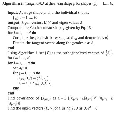
The Karcher mean captures the characteristic corpus callosum shape for a given population. It also serves as a common reference template for registering the individual shapes to perform a group analysis. Instead of being a subject-specific template, it is a statistical template that minimizes the shape variance during its reconstruction. The main advantage of this approach is that it also allows us to explore the covariance structure of the corpus callosum shapes in an intrinsic manner. Using the inverse exponential maps given by Eq. 17, we can represent each individual shape q_i in the shape space by its tangent vector ${{\alpha }_t}^i$ from the mean shape μ. Thus for a collection of N shapes, we compute geodesics from the mean shape to each individual and represent their tangent vectors as $\left\{{{\alpha }_t}^i\right\},i=1,\dots ,N$. Fig. 6 shows a schematic of this process where the geodesics from the mean shape μ to an individual shape q_i are represented by tangent vectors in the Euclidean space $T_{\mu }\left(\mathcal{S}\right)$. The tangent space $T_{\mu }\left(\mathcal{S}\right)$ can be represented using a Fourier basis. To derive a covariance structure for the population, we first orthogonalize the tangent vectors using the Gram Schmidt (Golub and Van Loan, 1996) process to obtain a set of orthogonalized tangent vectors denoted by {Y_i},i=1,…,N. The Gram Schmidt process uses the Riemannian metric on the tangent space and is described in Algorithm 1 for completeness.

Fig. 6.

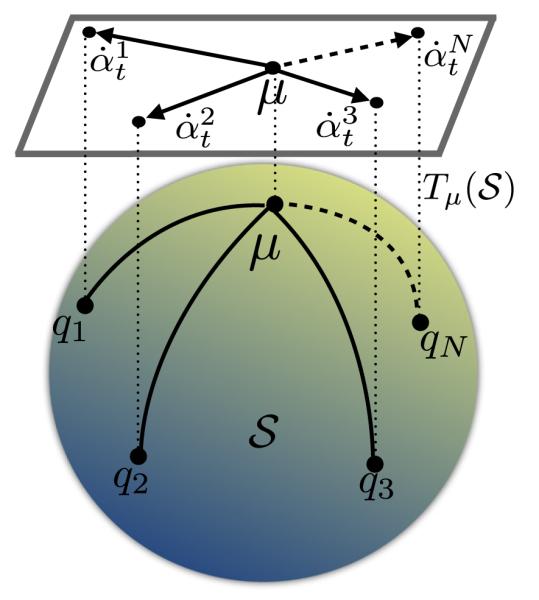
Projection of geodesics from the shape space S to the tangent space T_μ(S) at the mean shape μ.

The orthogonalized tangent vectors form a tangent space basis at the mean shape for the population. To reduce their dimensions for statistical analysis, we first project the tangent vectors to the orthogonal basis and compute the covariance matrix of the projections. For a tangent vector ${{\alpha }_t}^i$, its projection to the orthogonal basis is given by

$$X_{\mathrm{proj}}^i=\sum _{j=1}^N\langle {{\stackrel{.}{\alpha }}_t}^i,Y_j\rangle Y_j,i=1,\dots ,N.$$ (19)

We then compute the covariance matrix $\mathcal{C}$ as

$$\mathcal{C}=E\left[{\left(X_{\mathrm{proj}}-E\left[X_{\mathrm{proj}}\right]\right)}^T\left(X_{\mathrm{proj}}-E\left[X_{\mathrm{proj}}\right]\right)\right]$$ (20)

and compute the singular value decomposition to obtain the principal eigen vectors and eigen values as

$$\mathcal{C}={\mathit{USV}}^T.$$ (21)

The eigen vectors of the matrix $\mathcal{C}$ given by {U_i},i=…k,k⪡N form the basis of the reduced dimensional subspace at the mean shape μ. Fig. 7 illustrates this procedure using a schematic. It shows the mean shape μ and the tangent vectors to the individual shapes in the top panel. The middle panel of Fig. 7 shows the orthogonalized tangent vectors, whereas the bottom panel shows the eigen vectors after the TPCA decomposition. Algorithm 2 describes this procedure in detail. The set of k eigen vectors {U_i},i=1,…,k,k⪡N captures the callosal shape variability in the population. The choice of k is determined empirically by observing the decay in the variance captured by the eigen vectors. Finally for the purpose of statistical analysis each shape covariate is represented by the projection of the tangent vectors on the k-dimensional eigen basis in the tangent space. For a single eigen projection j, the scalar value $e_j^i$ represents the observation for shape i and is given by

$$e_j^i={\left(X_{\mathrm{proj}}^i\right)}^T{U}_j,j=1,\dots ,k.$$ (22)

Fig. 7.

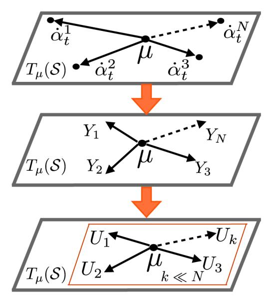
Illustration of the TPCA procedure. Top: original tangent vectors from the mean shape to individuals on the tangent space. Middle: orthogonalized tangent vectors on the tangent space. Bottom: principal eigen vectors after TPCA decomposition.

Shape synthesis and reconstruction

To visually verify that the TPCA model does indeed capture the underlying shape variability, we reconstruct eigen shapes from the model for prominent eigen directions, and find the corresponding native corpus callosum shapes closest to the eigen projections. Algorithm 3 presents the procedure for reconstructing eigen shapes as well as the closest original shapes in the population from a TPCA model for a given eigen direction.

Results

In this section, we present results from the statistical analysis performed to assess the shape variation of the corpus callosum in association with sex, age, schizophrenia and genetic predisposition for schizophrenia.

Data

The population data included structural MRI scans from 218 subjects enrolled in the UCLA Family Study (Nuechterlein et al., 2002; Yang et al., 2010) (age: 39.16±16 years, sex: 116 males, 102 females) – obtained after approval by the UCLA Institutional Review Board (IRB). Specifically, the subjects included 48 patients with a DSM-IV diagnosis of schizophrenia (36 M/13 F; mean age: 31.8±8.9 SD), 66 unaffected first-degree relatives of patients (29 M/41 F; 46.84±16.13), and 104 community comparison (C) subjects and their first-degree relatives (50 M/55 F; 37.52±16.53) sampled from 96 separate families. Table 2 shows the demographic and clinical details of subjects. Groups defined by biological risk for schizophrenia (schizophrenia patients, patient relatives and controls) differed in age (F(5, 215)=15.04, p<.001) and gender (χ²(5, 215)=11.56, p<.001), but not handedness or years of education completed. These subjects underwent high-resolution T1-weighted structural MRI scanning on a Siemens 1.5 T Sonata system using a 3D MPRAGE sequence (FOV= 256; TR/TE=1900 ms/28 ms; voxel size=1 mm×1 mm×1 mm; TI=1100; matrix size=256×256×160; flip angle: 15°, averages: 4). The corpus callosum was manually contoured on the sagittal slices for each subject. Intra and inter-rater reliability for manual tracing, determined by repeat contouring of the callosum in six randomly chosen brain volumes, was r₁>0.98. Additionally, using the parcellation scheme provided by Freesurfer, the callosum was also separated into five subregions to determine the effects of sex, age and schizophrenia for midsagittal callosal area.

Table 2.

Demographic and MRI measures for schizophrenia patients, non-psychotic relatives of patients, C (community comparison) probands, and non-psychotic relatives of C probands

	Schizophrenia patients		Patient relatives				C probands		Relatives of C probands
			Siblings		Parents				Siblings		Parents
	(N=48)		(N=24)		(N=42)		(N=27)		(N=38)		(N=39)
	Mean	SD	Mean	SD	Mean	SD	Mean	SD	Mean	SD	Mean	SD
Demographic measures
Age (years)a	31.8	9.0	31.8	13.3	55.6	9.6	26.4	7.1	26.9	9.4	56.1	8.0
Handedness (L/R)	4/44		2/22		3/39		2/25		1/37		3/36
Gender (M/F)a	35/13		13/11		14/28		19/8		18/20		17/22
MRI measures (cm3)
Brain volumea	1427.3	135.9	1408.7	153.6	1329.8	148.7	1398.4	114.5	1418.0	164.7	1381.8	152.8
Gray matter volumea,b	667.1	42.4	677.0	42.0	625.8	42.4	707.3	38.1	709.0	41.3	618.7	45.0
White matter volumea,b	537.5	35.0	532.8	39.7	544.6	37.9	517.0	24.1	511.5	34.9	536.9	34.1

^aIndicates significant group difference.

^bDenotes that volumes were corrected for total brain volume, sex and age.

Mean shapes for population

The procedures described in the Karcher mean section were applied to the corpus callosum traces for healthy controls, schizophrenia patients, and all of the subjects together. The resulting mean shapes are displayed in Fig. 8, where the top panels show the mean shapes for each group separately and the bottom panel shows the three mean shapes overlaid for better comparison. The callosal shapes for healthy controls appear flatter, whereas those for the schizophrenia patients are more arched.

Fig. 8.

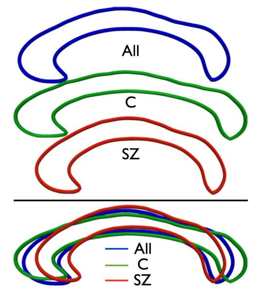
Top panel: mean shapes for all subjects, controls, and schizophrenia patients. Bottom panel: mean shapes overlaid on each other.

TPCA variation

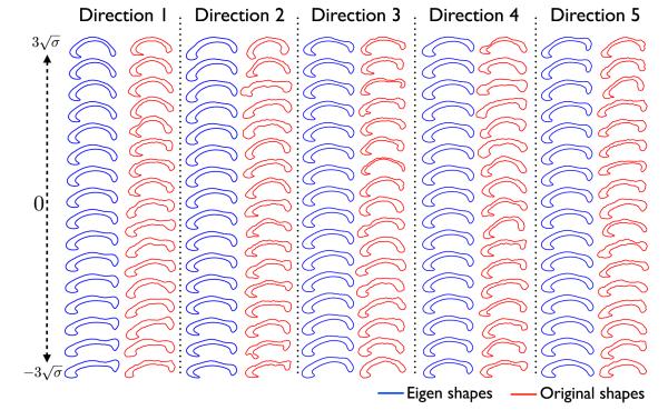
Visualization of the group mean shapes of the different subsets is qualitative and not instructive about the directions in the underlying shape variation in the population. To analyze the covariance structure of shapes, we applied the tangent principal component analysis described in the Tangent space PCA for shapes section above. The first ten (k=10) eigen-projections (accounting for around 70% of the variance) were included as shape covariates for each subject for subsequent statistical analysis. The cut-off choice k=10 was chosen to reduce the possibility of type II errors for the statistical analysis. The distribution of the eigen values was heavy-tailed, suggesting that the shape analysis method was highly sensitive to local changes in shape. Algorithm 3 above was used to visualize the eigen shape variation from the TPCA model. Fig. 9 shows the eigen shape variation for ±3 standard deviations about the mean shape, as well as the closest corresponding original shapes from the population for the first five eigen directions. As illustrated in this figure, each direction captures specific morphological characteristics of the underlying population shape variation. For example, going from top to bottom, the first eigen mode reflects arching of the corpus callosum and also the extent to which the splenium is bulbous in shape. The second eigen mode reflects the shape of the genu becoming more bulbous, when going from bottom to top. The closest original shapes corresponding to the eigen shapes exhibit similar morphological variation thus confirming that the TPCA model captures salient shape characteristics in the population. To visualize the effect of the extreme eigen shape variation, Fig. 10 overlays the eigen shapes at the two extremities $(\pm 3\sqrt{\sigma })$.

Fig. 9.

Eigen shape variation and the corresponding variation of the original shapes in the population for ±3 standard deviations about the mean shape for eigen directions 1–5.

Fig. 10.

Eigen shapes at the two extremities $(\pm 3\sqrt{\sigma })$ overlaid on top of each other.

Mixed effects modeling

Linear regression and mixed model analyses were used to examine genetic-liability effects by comparing schizophrenia patients, relatives of patients, and control subjects and their relatives. To examine effects of schizophrenia, patients with schizophrenia were compared to community comparison subjects and their relatives. Sex and age were included as covariates in all statistical analyses. Since some subjects were biologically related, family membership was included as a random factor for all analyses including related individuals. Significant schizophrenia effects were followed-up by examining effects of disease-related genetic liability (comparing patient relatives to controls) and disease-specific processes (comparing patients and patient relatives) in pairwise contrasts. Examining the first five PCA sources describing callosal shape variation, significant sex effects were observed for the first (p=0.04), second (p=0.014), and the third (p=0.025) eigen projections. Significant age effects were observed for the first and the fourth eigen projections (p<0.0001). Significant schizophrenia effects (schizophrenia patients versus C subjects) were observed for the first eigen projection (p=0.023). Additionally, the first eigen projection showed a significant disease-specific effect (p=0.004) when schizophrenia probands were compared with non-psychotic first-degree relatives of patients. The third eigen projection showed both significant genetic liability effects (p=0.021) when non-psychotic patient siblings were compared to healthy control probands and siblings, as well as disease-specific effects (p=0.019). The statistical results highlighting main effects for age, sex, and schizophrenia are summarized in Table 3.

Table 3.

Summary of significant main effects (highlighted in red) for age, sex, schizophrenia (patients compared to controls and control relatives), genetic liability (patient relatives compared to controls and control relatives) and disease-related effects (patients compared to patient relatives).^a

	Sex		Age		Schizophrenia effect		Genetic liability effect		Disease-specific effect
					Patients vs controls		Patient relatives vs controls		Patients vs patient relatives
	F	p	F	p	t	p	t	p	t	p
PCA 1	8.37	0.04	12.85	< 0.0001	−2.30	0.023	0.65	0.599	−2.90	0.004
PCA 2	6.10	0.014	0.033	0.855	−0.99	0.326	0.05	0.960	−0.98	0.329
PCA 3	5.07	0.025	1.67	0.198	0.29	0.765	2.35	0.021	2.37	0.019
PCA 4	2.39	0.124	41.52	< 0.0001	0.87	0.385	−1.63	0.110	−0.74	0.459
PCA 5	1.04	0.310	0.70	0.404	−0.48	0.636	−0.48	0.633	−0.01	0.990

^aNegative values of t indicate patients>controls, patient relatives>controls, and patients>patient relatives

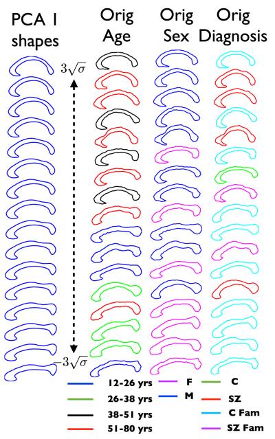
To visualize the corpus callosum shape variation related to sex, age, and biological risk for schizophrenia, we color-coded the original shapes closest to the first eigen projection according to their gender, age, and diagnosis (Fig. 11). Subject age was divided into four quartiles over the total age range of 12–80 years, while diagnosis was coded according to whether a subject was a healthy control, a control relative, a schizophrenia patient, or a patient relative. From Fig. 11, we observe that the tail end of the first eigen projection indicated that older male subjects and predominantly patients were more likely to show an arching of the callosum.

Fig. 11.

Original shape variation in the population along eigen direction 1, color coded according to age, sex, and diagnosis. The eigen shape variation is displayed in the first column for comparison.

To determine the effect of sex, age and diagnosis on local shape changes in the corpus callosum, we chose the first eigen projection and reconstructed the callosal shapes using Algorithm 3 described above. Since the shape is reconstructed from the average, we computed the magnitude of the deformation field from the mean shape to the generated shape. This deformation field is computed at each poin talong the shape and thus represents a local measure of distortion of the shape about the mean. We then used the general linear model at each point to test the main effects of sex, age, and biological risk for schizophrenia on the local changes in shape, including each of the other remaining covariates in the model. We found significant effects for both sex and age for the local shape changes reflected in the deformation field due to the first eigen direction. Additionally, we analyzed the residual contributions for eigen projections 2–10 using the same statistical model including false discovery rate (FDR) correction. Significant age (p_FDR=0.00018) and sex (p_FDR=0.0043) effects were found locally along the shape for the first eigen projection. We also found significant age (p_FDR=0.0052) and sex (p_FDR=0.00625) effects for local shape when analyzing the residual variation for the remaining (2–10) eigen projections. Though some locations showed significant effects of diagnosis, the results did not survive the threshold for multiple comparisons. Fig. 12 shows the significant p-values overlaid on the mean shape for sex and age for the first eigen projection as well as the residual (2–10) projections. While we observe significant effects due to sex almost all over the shape for the dominant eigen projection, the effects are localized to the genu and partially to the splenium for age.

Fig. 12.

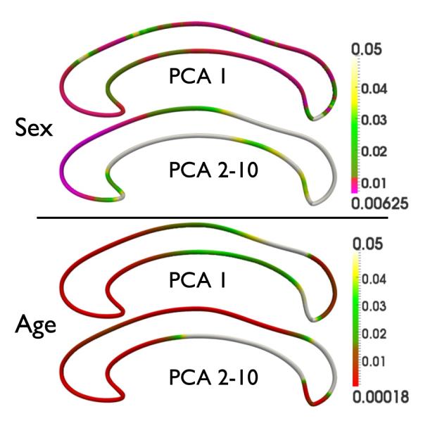
Significant local shape changes in the corpus callosum for sex (top panel), and age (bottom panel). Results are corrected for multiple comparisons by thresholding with FDR.

Comparison with callosal thickness

We computed the local thickness (see Luders et al., 2010; Narr et al., 2000; Nasrallah et al., 1986 for the description of methods) of the callosal shape and projected it at each point along the contour. We used the same models previously used for the analysis of local deformation fields for analyzing thickness, but we failed to find any significant effects for sex, age and biological risk for schizophrenia.

Comparison with regional callosal areas

We compared our results with previously established regional measures of callosal anatomy by partitioning the corpus callosum into the posterior, mid-posterior, central, mid-anterior, and the anterior regions using Freesurfer (Dale et al., 1999). The regional areas as well as the total callosal area that have been used in prior studies in schizophrenia (Downhill et al., 2000) were measured for each subject. We used the same statistical models to examine sex, age, and schizophrenia effects and biological risk for the total and partitioned callosal areas. Whole brain and tissue volume measurements were also compared for descriptive purposes. Only significant age effects for the mid-anterior (p<0.0001), central (p<0.0001), the mid-posterior (p=0.001), and the total area (p=0.012) were observed. Without correction for brain volume, males had larger callosal areas than females (p<0.0001).

Shape correlation with sub-regional callosal areas

We also assessed the relationship of the intrinsic statistical shape covariates with the callosal area measures across the population. Significant associations were observed between the posterior region and the scores from the first (r=0.191, p=0.005), sixth (r=0.196, p=0.004), seventh (r=0.319, p<1e–5), and the eighth (r=−0.159, p=0.0019) eigen projections. In particular, eigen projection four was significantly correlated with the mid-posterior (r=−0.420, p<1e–5), central (r=−0.289, p<1e–5), mid-anterior (r=−0.3, p<1e–5), and anterior (r=−0.338, p<1e–5) regions as well as the total area (r=−0.354, p<1e–5). Similarly we observed significant correlations for the remaining regions with scores from multiple eigen shape projections as shown in Table 4. Importantly we also observed significant correlations of total white matter volume with the first (r=0.168, p=0.013), fourth (r=−0.201, p=0.003), and the tenth (r=0.138, p=0.042) eigen projections, as well as significant correlations of the cerebrospinal fluid (CSF) volume with the second (r=−0.249, p<1e–5), third (r=−0.221, p=0.001), fourth (r=0.179, p=0.008), and the ninth (r=−0.196, p=0.004) eigen shape projections.

Table 4.

Summary of significant (highlighted in red) correlations of eigen shape projections with corpus callosum regional areas

		PCA 1	PCA 2	PCA 3	PCA 4	PCA 5	PCA 6	PCA 7	PCA 8	PCA 9	PCA 10
Posterior	r	0.191	0.054	−0.019	−0.103	−0.071	0.196	0.319	−0.159	−0.020	0.110
	p	0.005	0.424	0.785	0.131	0.293	0.004	< 0.00001	0.019	0.767	0.106
Mid posterior	r	−0.069	0.041	0.068	−0.420	0.169	−0.015	−0.132	−0.034	0.266	0.002
	p	0.309	0.543	0.318	< 0.00001	0.013	0.831	0.051	0.613	< 0.00001	0.971
Central	r	−0.336	0.07	0.215	−0.289	0.138	0.076	−0.141	−0.032	0.155	0.062
	p	< 0.00001	0.298	0.001	< 0.00001	0.042	0.263	0.08	0.636	0.022	0.362
Mid anterior	r	−0.038	0.076	0.134	−0.300	0.000	0.055	−0.137	−0.048	0.154	−0.019
	p	0.578	0.267	0.048	< 0.00001	0.996	0.421	0.043	0.481	0.023	0.784
Anterior	r	0.295	−0.228	−0.054	−0.338	−0.200	0.106	−0.269	0.069	0.081	−0.05
	p	< 0.00001	0.001	0.425	< 0.00001	0.003	0.118	< 0.00001	0.311	0.236	0.459
Total area	r	0.041	−0.014	0.072	−0.354	−0.12	0.115	−0.264	−0.049	0.145	0.027
	p	0.545	0.838	0.291	< 0.0001	0.855	0.090	< 0.00001	0.475	0.033	0.687

Discussion and conclusion

We have presented a computational approach for the shape analysis of corpus callosum curves. The shape analysis framework uses the square-root velocity (Joshi et al., 2007a, 2007b) parameterization for continuous closed callosal curves and constructs a shape space of such representations. The shape analysis is invariant to common confounds such as rigid motions, scale and reparameterizations due to placement of the starting point, and changes in speed. This differential geometric framework for corpus callosum shape representation and matching naturally provides the means to perform intrinsic statistical analysis on the shape space. A Riemannian metric is induced on the shape space via its tangent space, and callosal geodesics are computed under this metric. Our work therefore provides, i) an invariant representation of the callosal shape boundary, ii) an intrinsic framework for statistical shape analysis, and iii) an intrinsic framework for population dimension reduction using PCA on the tangent space of shapes. While the choice of PCA including the Fourier basis for representing the tangent space was made for computational convenience, it is important to note that PCA yields a basis that maximizes the feature variance in the population along each projection. The maximization of shape variance does not explicitly encode discriminatory rules that classify the data. Additionally, even if the shape analysis is performed locally on the boundary, the principal component projections capture global shape properties in the data, and hence need to be interpreted appropriately. However it should be noted that the method is not restricted to the choice of PCA as the reduced dimensional basis for shapes. In the future, one could use a wavelet basis with a nonuniform energy compaction in conjunction with independent component analysis (ICA) for dimension reduction that can result in even more efficient representation.

The application of our analysis to a sizable population of shapes demonstrates both global and local effects of age, sex and biological risk status for schizophrenia on corpus callosum shape variation. Specifically, we show that callosal shape profiles predict individual differences in age, and sex and disease status that are independent of callosal size. Though to a lesser extent, variations in callosal shape were also shown to be associated with schizophrenia and genetic liability for schizophrenia. Age-related variations in callosal shape reflect a pronounced narrowing and arching of the corpus callosum with increasing age (Fig. 11), in addition to changes in other local shape characteristics. These observations may correspond to widely reported reductions in the callosal area and changes in white matter integrity measured with diffusion tensor imaging (DTI), which occur during mid and late adulthood (e.g. Hasan et al., 2008). Our findings also show differences in callosal shape in males and females. These observations are compatible with early reports suggesting that females exhibit a more bulbous splenium (DeLacoste-Utamsing and Holloway, 1982), though our results also indicate more rounded anterior aspects of the corpus callosum in females (Fig. 11). Statistical shape analysis also showed significant effects of schizophrenia and schizophrenia-related genetic vulnerability. However, age (see Figs. 11 and 12) appears to exhibit larger and more distributed effects on callosal shape than on biological risk for schizophrenia. These findings are in line with previous reports using linear and curvature measurements to show more bowing of the corpus callosum particularly in male patients as well as provide additional support to the idea that callosal shape may indicate genetic risk for schizophrenia (Narr et al., 2000, 2002). In this study, we compared our results with established corpus callosum morphometry measures such as local thickness and regional areas. The analysis of thickness failed to find significant differences in the population for sex, age, or biological risk for schizophrenia after controlling for brain size; only age effects were observed for callosal areas. These findings agree with prior studies of healthy adults (Luders et al., 2006), though findings in schizophrenia remain mixed (e.g., Narr et al., 2000; Nasrallah et al., 1986; Woodruff et al., 1995). While our shape measures showed significant correlations with the regional callosal areas, observations of shape variations reflecting a more bowed corpus callosum in male patients with schizophrenia as well as more subtle schizophrenia genetic liability effects are in line with previous reports using linear and curvature measurements (Narr et al., 2000, 2002). Cumulatively these results suggest that our method, which allows for a detailed morphological characterization of callosal shape, provides a more sensitive approach for dissociating individual differences in age, sex and clinical status.

References

- Aboitiz F, Scheibel A, Fisher R, Zaidel E. Fiber composition of the human corpus callosum. Brain Res. 1992;598(1–2):143–153. doi: 10.1016/0006-8993(92)90178-c. [DOI] [PubMed] [Google Scholar]
- Adamson CL, Wood AG, Chen J, Barton S, Reutens DC, Pantelis C, Velakoulis D, Walterfang M. Thickness profile generation for the corpus callosum using Laplace’s equation. Hum. Brain Mapp. 2011;32(12):2131–2140. doi: 10.1002/hbm.21174. [DOI] [PMC free article] [PubMed] [Google Scholar]
- Bhattacharya R, Patrangenaru V. Nonparametric estimation of location and dispersion on Riemannian manifolds. J. Stat. Plann. Inference. 2002;108(1–2):23–35. [Google Scholar]
- Bodensteiner J, Schaefer G, Breeding L, Cowan L. Hypoplasia of the corpus callosum: a study of 445 consecutive MRI scans. J. Child Neurol. 1994;9(1):47–49. doi: 10.1177/088307389400900111. [DOI] [PubMed] [Google Scholar]
- Bookstein FL, Sampson PD, Connor PD, Streissguth AP. Midline corpus callosum is a neuroanatomical focus of fetal alcohol damage. Anat. Rec. Adv. Integr. Anat. Evol. Biol. 2002a;269(3):162–174. doi: 10.1002/ar.10110. [DOI] [PubMed] [Google Scholar]
- Bookstein FL, Streissguth AP, Sampson PD, Connor PD, Barr HM. Corpus callosum shape and neuropsychological deficits in adult males with heavy fetal alcohol exposure. Neuroimage. 2002b;15(1):233–251. doi: 10.1006/nimg.2001.0977. [DOI] [PubMed] [Google Scholar]
- Bookstein FL, Connor PD, Huggins JE, Barr HM, Pimentel KD, Streissguth AP. Many infants prenatally exposed to high levels of alcohol show one particular anomaly of the corpus callosum. Alcohol. Clin. Exp. Res. 2007;31(5):868–879. doi: 10.1111/j.1530-0277.2007.00367.x. [DOI] [PubMed] [Google Scholar]
- Brigger P, Hoeg J, Unser M. B-spline snakes: a flexible tool for parametric contour detection. IEEE Trans. Image Process. 2000;9(9):1484–1496. doi: 10.1109/83.862624. [DOI] [PubMed] [Google Scholar]
- Clarke J, Zaidel E. Anatomical-behavioral relationships: corpus callosum morphometry and hemispheric specialization. Behav. Brain Res. 1994;64(1–2):185–202. doi: 10.1016/0166-4328(94)90131-7. [DOI] [PubMed] [Google Scholar]
- Dale AM, Fischl B, Sereno MI. Cortical surface-based analysis. I. Segmentation and surface reconstruction. Neuroimage. 1999;9(2):179–194. doi: 10.1006/nimg.1998.0395. [DOI] [PubMed] [Google Scholar]
- DeLacoste-Utamsing C, Holloway R. Sexual dimorphism in the human corpus callosum. Science. 1982;216(4553):1431–1432. doi: 10.1126/science.7089533. [DOI] [PubMed] [Google Scholar]
- Downhill J, Buchsbaum M, Wei T, Spiegel Cohen J, Hazlett E, Haznedar M, Silverman J, Siever L. Shape and size of the corpus callosum in schizophrenia and schizotypal personality disorder. Schizophr. Res. 2000;42(3):193–208. doi: 10.1016/s0920-9964(99)00123-1. [DOI] [PubMed] [Google Scholar]
- Dutt A, Shaikh M, Ganguly T, Nosarti C, Walshe M, Arranz M, Rifkin L, McDonald C, Chaddock C, McGuire P, et al. COMT gene polymorphism and corpus callosum morphometry in preterm born adults. Neuroimage. 2011;54(1):148–153. doi: 10.1016/j.neuroimage.2010.07.048. [DOI] [PubMed] [Google Scholar]
- El-Baz A, Elnakib A, Casanova M, GimelÕfarb G, Switala A, Jordan D, Rainey S. Accurate automated detection of autism related corpus callosum abnormalities. J. Med. Syst. 2011;35(5):929. doi: 10.1007/s10916-010-9510-3. [DOI] [PubMed] [Google Scholar]
- Fletcher P, Joshi S. Principal geodesic analysis on symmetric spaces: statistics of diffusion tensors. Comput. Vision Math. Methods Med. Biomed. Image Anal. 2004;3117:87–98. [Google Scholar]
- Frazier T, Hardan A. A meta-analysis of the corpus callosum in autism. Biol. Psychiatry. 2009;66(10):935–941. doi: 10.1016/j.biopsych.2009.07.022. [DOI] [PMC free article] [PubMed] [Google Scholar]
- Golub G, Van Loan C. Matrix Computations. vol. 3. Johns Hopkins Univ Pr.; 1996. [Google Scholar]
- Guo H, Rangarajan A, Joshi S, Younes L. Non-rigid registration of shapes via diffeomorphic point matching. IEEE International Symposium on Biomedical Imaging: Nano to Macro. IEEE. 2004:924–927. [Google Scholar]
- Hasan K, Kamali A, Kramer L, Papnicolaou A, Fletcher J, Ewing-Cobbs L. Diffusion tensor quantification of the human midsagittal corpus callosum subdivisions across the lifespan. Brain Res. 2008;1227:52–67. doi: 10.1016/j.brainres.2008.06.030. [DOI] [PMC free article] [PubMed] [Google Scholar]
- Hofer S, Frahm J. Topography of the human corpus callosum revisited–comprehensive fiber tractography using diffusion tensor magnetic resonance imaging. Neuroimage. 2006;32(3):989–994. doi: 10.1016/j.neuroimage.2006.05.044. [DOI] [PubMed] [Google Scholar]
- Innocenti G, Ansermet F, Parnas J. Schizophrenia, neurodevelopment and corpus callosum. Mol. Psychiatry. 2003;8(3):261–274. doi: 10.1038/sj.mp.4001205. [DOI] [PubMed] [Google Scholar]
- John J, Shakeel M, Jain S. Corpus callosal area differences and gender dimorphism in neuroleptic-naive, recent-onset schizophrenia and healthy control subjects. Schizophr. Res. 2008;103(1–3):11–21. doi: 10.1016/j.schres.2008.04.035. [DOI] [PMC free article] [PubMed] [Google Scholar]
- Joshi SH, Klassen E, Srivastava A, Jermyn I. A novel representation for Riemannian analysis of elastic curves in Rn. Proceedings of the IEEE Computer Society Conference on Computer Vision and Pattern Recognition. 2007a:1–7. doi: 10.1109/CVPR.2007.383185. [DOI] [PMC free article] [PubMed] [Google Scholar]
- Joshi SH, Klassen E, Srivastava A, Jermyn I. Energy Minimization Methods in Computer Vision and Pattern Recognition. Springer; 2007b. Removing shape-preserving transformations in square-root elastic (SRE) framework for shape analysis of curves; pp. 387–398. [DOI] [PMC free article] [PubMed] [Google Scholar]
- Kendall B. Dysgenesis of the corpus callosum. Neuroradiology. 1983;25(4):239–256. doi: 10.1007/BF00540236. [DOI] [PubMed] [Google Scholar]
- Knöchel C, Oertel-Knöchel V, Schönmeyer R, Rotarska-Jagiela A, van de Ven V, Prvulovic D, Haenschel C, Uhlhaas P, Pantel J, Hampel H, Linden DE. Interhemispheric hypoconnectivity in schizophrenia: Fiber integrity and volume differences of the corpus callosum in patients and unaffected relatives. Neuroimage. 2012;59(2):926–934. doi: 10.1016/j.neuroimage.2011.07.088. [DOI] [PubMed] [Google Scholar]
- Le H. Mean size-and-shapes and mean shapes: a geometric point of view. Adv. Appl. Probab. 1995;27(1):44–55. [Google Scholar]
- Le H. Locating Fréchet means with application to shape spaces. Adv. Appl. Probab. 2001;33(2):324–338. [Google Scholar]
- Luders E, Narr K, Zaidel E, Thompson P, Toga A. Gender effects on callosal thickness in scaled and unscaled space. Neuroreport. 2006;17(11):1103–1106. doi: 10.1097/01.wnr.0000227987.77304.cc. [DOI] [PubMed] [Google Scholar]
- Luders E, Narr K, Bilder R, Thompson P, Szeszko P, Hamilton L, Toga A. Positive correlations between corpus callosum thickness and intelligence. Neuroimage. 2007;37(4):1457–1464. doi: 10.1016/j.neuroimage.2007.06.028. [DOI] [PMC free article] [PubMed] [Google Scholar]
- Luders E, Narr K, Hamilton L, Phillips O, Thompson P, Valle J, Del’Homme M, Strickland T, McCracken J, Toga A, et al. Decreased callosal thickness in attention-deficit/hyperactivity disorder. Biol. Psychiatry. 2009;65(1):84–88. doi: 10.1016/j.biopsych.2008.08.027. [DOI] [PMC free article] [PubMed] [Google Scholar]
- Luders E, Thompson P, Toga A. The development of the corpus callosum in the healthy human brain. J. Neurosci. 2010;30(33):10985–10990. doi: 10.1523/JNEUROSCI.5122-09.2010. [DOI] [PMC free article] [PubMed] [Google Scholar]
- Luders E, Thompson P, Narr K, Zamanyan A, Chou Y, Gutman B, Dinov I, Toga A. The link between callosal thickness and intelligence in healthy children and adolescents. Neuroimage. 2011;54(3):1823–1830. doi: 10.1016/j.neuroimage.2010.09.083. [DOI] [PMC free article] [PubMed] [Google Scholar]
- Narr K, Thompson P, Sharma T, Moussai J, Cannestra A, Toga A. Mapping morphology of the corpus callosum in schizophrenia. Cereb. Cortex. 2000;10(1):40–49. doi: 10.1093/cercor/10.1.40. [DOI] [PubMed] [Google Scholar]
- Narr K, Cannon T, Woods R, Thompson P, Kim S, Asunction D, van Erp T, Poutanen V, Huttunen M, Lönnqvist J, et al. Genetic contributions to altered callosal morphology in schizophrenia. J. Neurosci. 2002;22(9):3720–3729. doi: 10.1523/JNEUROSCI.22-09-03720.2002. [DOI] [PMC free article] [PubMed] [Google Scholar]
- Nasrallah H, Andreasen N, Coffman J, Olson S, Dunn V, Ehrhardt J, Chapman S. A controlled magnetic resonance imaging study of corpus callosum thickness in schizophrenia. Biol. Psychiatry. 1986;21(3):274–282. doi: 10.1016/0006-3223(86)90048-x. [DOI] [PubMed] [Google Scholar]
- Nuechterlein K, Asarnow R, Subotnik K, Fogelson D, Payne D, Kendler K, Neale M, Jacobson K, Mintz J. The structure of schizotypy: relationships between neurocognitive and personality disorder features in relatives of schizophrenic patients in the UCLA Family Study. Schizophr. Res. 2002;54(1):121–130. doi: 10.1016/s0920-9964(01)00359-0. [DOI] [PubMed] [Google Scholar]
- Paul L, Brown W, Adolphs R, Tyszka J, Richards L, Mukherjee P, Sherr E. Agenesis of the corpus callosum: genetic, developmental and functional aspects of connectivity. Nat. Rev. Neurosci. 2007;8(4):287–299. doi: 10.1038/nrn2107. [DOI] [PubMed] [Google Scholar]
- Rajapakse J, Giedd J, Rumsey J, Vaituzis A, Hamburger S, Rapoport J. Regional MRI measurements of the corpus callosum: a methodological and developmental study. Brain Dev. 1996;18(5):379–388. doi: 10.1016/0387-7604(96)00034-4. [DOI] [PubMed] [Google Scholar]
- Riise J, Pakkenberg B. Stereological estimation of the total number of myelinated callosal fibers in human subjects. J. Anat. 2011;218(3):277–284. doi: 10.1111/j.1469-7580.2010.01333.x. [DOI] [PMC free article] [PubMed] [Google Scholar]
- Rohlf F, Slice D. Extensions of the Procrustes method for the optimal superimposition of landmarks. Syst. Biol. 1990;39(1):40–59. [Google Scholar]
- Rotarska-Jagiela A, Schönmeyer R, Oertel V, Haenschel C, Vogeley K, Linden D. The corpus callosum in schizophrenia-volume and connectivity changes affect specific regions. Neuroimage. 2008;39(4):1522–1532. doi: 10.1016/j.neuroimage.2007.10.063. [DOI] [PubMed] [Google Scholar]
- Srivastava A, Joshi S, Mio W, Liu X. Statistical shape analysis: clustering, learning, and testing. IEEE Trans. Pattern Anal. Mach. Intell. 2005;27(4):590–602. doi: 10.1109/TPAMI.2005.86. [DOI] [PubMed] [Google Scholar]
- Srivastava A, Klassen E, Joshi SH, Jermyn I. Shape analysis of elastic curves in euclidean spaces. IEEE Trans. Pattern Anal. Mach. Intell. 2011;33(7):1428–1451. doi: 10.1109/TPAMI.2010.184. [DOI] [PubMed] [Google Scholar]
- Thompson P, Narr K, Blanton R, Toga A. The Parallel Brain: The Cognitive Neuroscience of the Corpus Callosum. MIT Press; Cambridge, Massachusetts: 2003. Mapping structural alterations of the corpus callosum during brain development and degeneration; pp. 93–130. [Google Scholar]
- Vaillant M, Miller M, Younes L, Trouvé A. Statistics on diffeomorphisms via tangent space representations. Neuroimage. 2004;23:S161–S169. doi: 10.1016/j.neuroimage.2004.07.023. [DOI] [PubMed] [Google Scholar]
- Van Bon B, Koolen D, Borgatti R, Magee A, Garcia-Minaur S, Rooms L, Reardon W, Zollino M, Bonaglia M, De Gregori M, et al. Clinical and molecular characteristics of 1qter microdeletion syndrome: delineating a critical region for corpus callosum agenesis/hypogenesis. J. Med. Genet. 2008;45(6):346–354. doi: 10.1136/jmg.2007.055830. [DOI] [PubMed] [Google Scholar]
- Walterfang M, Yung A, Wood A, Reutens D, Phillips L, Wood S, Chen J, Velakoulis D, McGorry P, Pantelis C. Corpus callosum shape alterations in individuals prior to the onset of psychosis. Schizophr. Res. 2008;103(1–3):1–10. doi: 10.1016/j.schres.2008.04.042. [DOI] [PubMed] [Google Scholar]
- Weber B, Luders E, Faber J, Richter S, Quesada C, Urbach H, Thompson P, Toga A, Elger C, Helmstaedter C. Distinct regional atrophy in the corpus callosum of patients with temporal lobe epilepsy. Brain. 2007;130(12):3149–3154. doi: 10.1093/brain/awm186. [DOI] [PMC free article] [PubMed] [Google Scholar]
- Witelson S. Hand and sex differences in the isthmus and genu of the human corpus callosum. Brain. 1989;112(3):799–835. doi: 10.1093/brain/112.3.799. [DOI] [PubMed] [Google Scholar]
- Woodruff P, McManus I, David A. Meta-analysis of corpus callosum size in schizophrenia. J. Neurol. Neurosurg. Psychiatry. 1995;58(4):457–461. doi: 10.1136/jnnp.58.4.457. [DOI] [PMC free article] [PubMed] [Google Scholar]
- Woods R. Characterizing volume and surface deformations in an atlas framework: theory, applications, and implementation. Neuroimage. 2003;18(3):769–788. doi: 10.1016/s1053-8119(03)00019-3. [DOI] [PubMed] [Google Scholar]
- Yang Y, Nuechterlein K, Phillips O, Hamilton L, Subotnik K, Asarnow R, Toga A, Narr K. The contributions of disease and genetic factors towards regional cortical thinning in schizophrenia: the UCLA Family Study. Schizophr. Res. 2010;123(2–3):116–125. doi: 10.1016/j.schres.2010.08.005. [DOI] [PMC free article] [PubMed] [Google Scholar]
Associated Data
This section collects any data citations, data availability statements, or supplementary materials included in this article.