A GENERATIVE MODEL FOR MULTI-ATLAS SEGMENTATION ACROSS MODALITIES

Abstract

Current label fusion methods enhance multi-atlas segmentation by locally weighting the contribution of the atlases according to their similarity to the target volume after registration. However, these methods cannot handle voxel intensity inconsistencies between the atlases and the target image, which limits their application across modalities or even across MRI datasets due to differences in image contrast. Here we present a generative model for multi-atlas image segmentation, which does not rely on the intensity of the training images. Instead, we exploit the consistency of voxel intensities within regions in the target volume and their relation to the propagated labels. This is formulated in a probabilistic framework, where the most likely segmentation is obtained with variational expectation maximization (EM). The approach is demonstrated in an experiment where T₁-weighted MRI atlases are used to segment proton-density (PD) weighted brain MRI scans, a scenario in which traditional weighting schemes cannot be used. Our method significantly improves the results provided by majority voting and STAPLE.

1. INTRODUCTION

In traditional atlas-based segmentation[1, 2], a template volume (henceforth “atlas”) is registered (i.e. spatially aligned) to a target scan. The resulting deformation is then used to propagate the associated manual labels (either deterministic or probabilistic) and obtain the final segmentation. The main disadvantage of this technique is that a single deformation is limited in representing the whole population of potential target cases. This issue can be addressed by registering multiple atlases to the target volume. The question is then how to combine the “opinions” of different atlases. This problem is known as label fusion.

Majority voting[3], in which the mode of the propagated labels is selected as the final segmentation for each voxel, is widely used in medical imaging because it is straightforward to implement and, thanks to the maturity of registration methods, often yields good results. However, majority voting might not be able to correctly segment features that are present but underrepresented in the training dataset. STAPLE[4] weighs the propagated labels according to an estimated accuracy level, while incorporating consistency constraints. Neither majority voting nor STAPLE consider image intensities after registration. Higher segmentation accuracy can be achieved by considering the intensity of the images in label fusion, giving higher weights to the atlases which are more similar to the target volume, locally or globally[5, 6].

Weighted label fusion relies on the consistency of voxel intensities across scans. This represents a limitation in MRI, in which intensities depend heavily on the pulse sequence, acquisition settings and hardware. Mutual information has successfully been used for registration in such scenarios, but its inherent non-locality limits its application for local label fusion. Intensity normalization can ameliorate this problem, but only if the atlases and the target image are not acquired with different MRI contrast (e.g. T₁- vs. T₂-weighted).

Here we present a generative model for multi-atlas segmentation, which exploits the intensities of the target volumes by modeling their consistency within the regions to be segmented and their relation to the propagated labels. The intensities of the deformed templates are not considered in label fusion, so the set of atlases can include different modalities. As in [6], the registrations are assumed to be known (i.e. regarded as preprocessing), and we define a latent field that assigns each target voxel to a training volume. We assume that the image intensities for each label are samples from a Gaussian mixture model (GMM), modulated by a low-frequency bias field. Segmentation is formulated as finding the most likely labels in this framework. The algorithm is related to classical single atlas models[7], with two major differences: 1. we use a subject-specific prior probability for the labels computed in target space (as opposed to atlas space); and 2. the probabilistic model for the labels has a different structure.

2. METHODS

2.1. Generative Model

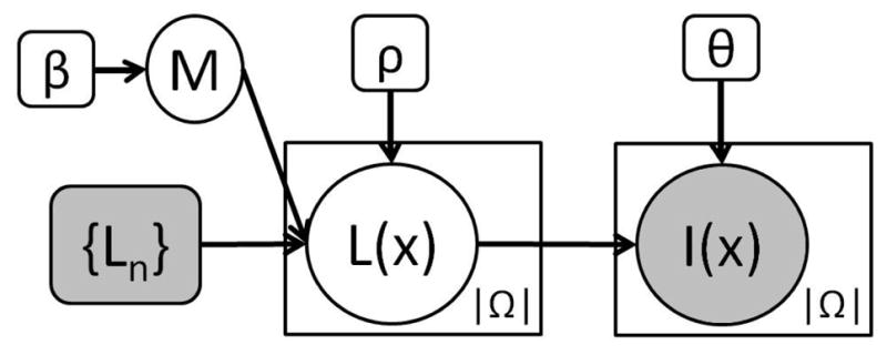
The generative model is depicted in Figure 1, and the corresponding equations are listed in Table 1. {L_n}, n = 1,…, N, represents the propagated labels from N available registered atlases. For a given voxel x ∈ Ω (where Ω is the image domain), L(x) is the underlying segmentation label we are trying to estimate, which takes discrete values between 1 and . L(x) is generated by the M(x)^th atlas through a logOdds model[8] (Equation 2 in Table 1). The slope ρ of the model is assumed to be fixed and known. $D_n^l(x)$ represents the signed distance transform for atlas n and label l.

Fig. 1.

Proposed graphical model. Plates indicate replication, shaded variables are observed.

Table 1.

Equations corresponding to the model in Figure 1.

$M~\frac{1}{Z(\beta )}{\prod }_{x\in \mathrm{\Omega }}exp\left(\beta {\sum }_{y\in {\mathcal{N}}_x}\delta (M(x)=M(y))\right)$ $L(x)~\frac{exp\left(\rho D_{M(x)}^{L(x)}(x)\right)}{{\sum }_{l^{\prime }=1}^{\mathcal{L}}exp\left(\rho D_{M(x)}^{l^{\prime }}(x)\right)}$ $I^{\ast }(x)~{\sum }_{k=1}^{{\mathcal{C}}_{L(x)}}\frac{w_{L(x),k}}{\sqrt{(2\pi {\sigma }_{L(x),k}^2)}}exp\left[-\frac{{(I^{\ast }(x)-{\mu }_{L(x),k})}^2}{2{\sigma }_{L(x),k}^2}\right]$ $I(x)=I^{\ast }(x)exp\left[-{\sum }_p{c}_p{\psi }_p(x)\right]$

The indices M(x) are not independent across voxels, but distributed according to a Markov Random Field (MRF) with smoothness parameter β (see Equation 1 in Table 1, where δ represents Kronecker’s delta and is the 6-neighborhood of voxel x). Now, given the labels L(x), the “true”, underlying intensities I* (x) are assumed to be samples of a GMM with components and parameters ${\mathrm{\Gamma }}_{L(x)}=\{\{w_{L(x),k}\},\{{\mu }_{L(x),k}\},\{{\sigma }_{L(x),k}^2\}\}$ (Equation 3 in Table 1). These underlying intensities are corrupted by a multiplicative bias field to yield the observed intensities I(x) (Equation 4 in the table, where {ψ_p(x)} is a set of spatially smooth basis functions). We use Θ to summarize all these image intensity parameters i.e., Θ = {{Γ_l}, {c_p}}. The bias field basis functions {ψ_p(x)}, as well as the parameters β and { } are assumed to be fixed and known. Note that the bias field is explicitly modeled as an exponential, which guarantees that it is greater than zero.

Some popular segmentation frameworks are particular cases of the proposed method. If β = 0, the model becomes very similar to a classical atlas-based segmentation method, e.g. [7], with the difference that here the label priors are built in subject space. Also, if β = ∞, the labels are generated only by the atlas that is closest to the target volume, which is close to best template selection. Another particular case of interest would be β = 0, ${\sigma }_{l,k}^2=\infty$, ∀l, k, in which case the algorithm simplifies to majority voting.

2.2. Segmentation

We formulate the segmentation as an optimization problem:

$$\begin{array}{l}\{\widehat{L},\widehat{\mathrm{\Theta }}\}=arg\underset{L,\mathrm{\Theta }}{max}p(L,\mathrm{\Theta }\mid I,\{L_n\})\\ =arg\underset{L,\mathrm{\Theta }}{max}log[p(I\mid L,\mathrm{\Theta })p(L\mid \{L_n\})]\end{array}$$

where we assume p(Θ) ∝ 1. We solve this problem using coordinate ascent, iteratively optimizing for L and Θ until convergence (often after 5–10 iterations).

2.2.1. Optimizing Θ for fixed L

The problem simplifies to Θ̂ = arg max_Θ log p(I|L, Θ). Again, we use coordinate ascent within this step, alternatively optimizing for the parameters of the GMMs {Γ_l} and the bias field {c_p}. Updating {Γ_l} is closed-form and amounts to computing sample means and variances (if = 1) or a simple 1-D EM algorithm if > 1 (we use = 1 for all labels except the background). To update {c_p}, setting the derivatives equal to zero leads to a nonlinear system of equations that has no closed-form solution. Instead we use a numerical gradient ascent scheme with line search.

2.2.2. Optimizing L for fixed Θ

Here the problem is:

$$\begin{array}{l}\widehat{L}=arg\underset{L}{max}log[p(I\mid L,\mathrm{\Theta })p(L\mid \{L_n\})]\\ =arg\underset{L}{max}log\left[p(I\mid L,\mathrm{\Theta })\sum _{M}p(L\mid M,\{L_n\})p(M)\right]\end{array}$$

which is intractable because M(x) includes interdependencies between neighboring voxels. Instead, we use variational EM to maximize a lower bound. Given that the Kullback- Leibler divergence KL(A,B) ≥ 0, we define:

$$\begin{array}{l}J=log[p(I\mid L,\mathrm{\Theta })p(L\mid \{L_n\})]-KL(q(M),p(M\mid I,\mathrm{\Theta },\{L_n\},L))\\ =H(q)+\sum _{M}q(M)logp(M,L,I\mid \mathrm{\Theta },\{L_n\})\end{array}$$

where H(A) represents the entropy and q(M) is an arbitrary distribution on M. To maximize J, we use the standard computational trick that q is constrained to have the structure: q(M) = Π_x∈Ω q_x(M(x)). Then, variational EM maximizes J by iterating between an expectation (E) step which updates q(M) and a maximization (M) step which optimizes L.

E step: in the E step, we look for the q(M) which maximizes J, which happens when the KL divergence between q(M) and the posterior p(M|I,Θ, {L_n}, L) is minimized:

$$\widehat{q}=arg\underset{q}{min}\sum _{M}q(M)log\frac{q(M)}{p(I,L\mid M,\mathrm{\Theta },\{L_n\})p(M)}$$

where p(L, I|Θ, {L_n}) is omitted because it does not depend on M or q. Now, given the structure of q(M) and also:

$$p(I,L\mid M,\mathrm{\Theta },\{L_n\})=\prod _{x\in \mathrm{\Omega }}p(I(x)\mid {\mathrm{\Gamma }}_{L(x)},\{c_p\})p(L(x)\mid L_{M(x)}(x))$$

it can be shown that the problem becomes:

$$\begin{array}{l}arg\underset{q}{min}{\mathbb{E}}_q[-logp(M)]+\sum _{x\in \mathrm{\Omega }}{\mathbb{E}}_{q_x}[log{q}_x(M(x))]-\dots \\ \dots -{\mathbb{E}}_{q_x}[logp(I(x)\mid {\mathrm{\Gamma }}_{L(x)},\{c_p\}+logp(L(x)\mid L_{M(x)}(x)))]\end{array}$$

with the constraint that q_x(m) lies on the probability simplex. Writing the Lagrangian, taking derivatives with respect to q_x and setting them to zero yields:

$$q_x(M(x))=e^{\lambda (x)}p(L(x)\mid L_{M(x)}(x))e^{{\sum }_{y\in {\mathcal{N}}_x}{q}_y(M(x))}$$

where λ(x) is the multiplier that ensures Σ_m q_x(m) = 1.

The equation can be solved with fixed point iterations.

M step: the goal of the M step is to maximize J with respect to L assuming q(M) constant. Since we can discard the term H(q), and because of the structure of q(M), the maximization can be carried out voxel by voxel using exhaustive search over labels:

$$\widehat{L}(x)=arg\underset{l}{max}\sum _{m=1}^N{q}_x(m)log[p(I(x)\mid {\mathrm{\Gamma }}_l,\{c_p\})p(l\mid L_m(x))]$$

As in most label fusion methods, the resulting label map is not guaranteed to preserve the topology of the different structures. However, this seldom happens in practice and can always be corrected with post-processing.

3. EXPERIMENTS AND RESULTS

3.1. Data

Two datasets (training and test) were used in this study. The test dataset consists of FLASH PD-weighted brain scans from eight healthy subjects (1.5T, TR=20ms, TE=min, α = 3°, 1 mm. isotropic voxels). A total of 36 structures were manually labeled using the protocol described in [9]. The human raters took advantage of higher contrast, co-registered T₁-weighted data that we did not use in this study. As in [6], we only used a representative subset of the 36 structures for evaluation in this study: white matter (WM), cerebral cortex (CT), lateral ventricle (LV), hippocampus (HP), thalamus (TH), caudate (CA), putamen (PU), pallidum (PA), and amygdala (AM).

The training dataset consists of 39 T₁-weighted brain MRI scans (MP-RAGE, 1.5T, TR=9.7ms, TE=4.ms, TI=20ms, α = 10°, 1 mm. isotropic resolution) and corresponding manual delineations of the same brain structures (same labeling protocol). We note that these are the same subjects that were used to construct the probabilistic segmentation atlas in FreeSurfer[10]. These scans were bias-field corrected and skull-stripped using FreeSurfer, and then ITK (www.itk.org) was used to register them to the PD-weighted data with a nonrigid transform (a grid of control points and b-splines) and mutual information as metric.

3.2. Experimental setup

We segmented the eight target volumes using majority voting, STAPLE, and the proposed method with β = 0 (local fusion) and β = 0.75, which represents the general case. We arbitrarily chose this value for β to match that from Sabuncu et al[6]. The same motivation was used to set ρ = 1. Three mixture components were used for the background class, and a single Gaussian for all other classes. The basis functions {ψ_p} were set to a third order polynomial, which in 3D yields 20 coefficients. We set the number of atlases to N = 15; the presented results are an average over five runs with different, randomly selected atlases from the pool of 38. The accuracy of the segmentation is evaluated using Dice scores ( $\mathit{Dice}(A,B)=\frac{2\mid A\cap B\mid }{\mid A\mid +\mid B\mid }$), and statistical significance is assessed with one-tailed, paired t-tests.

3.3. Results

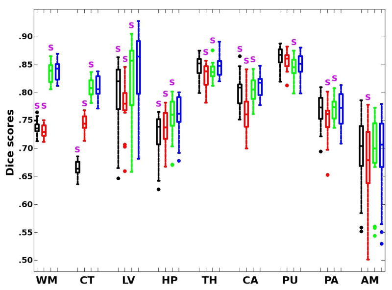
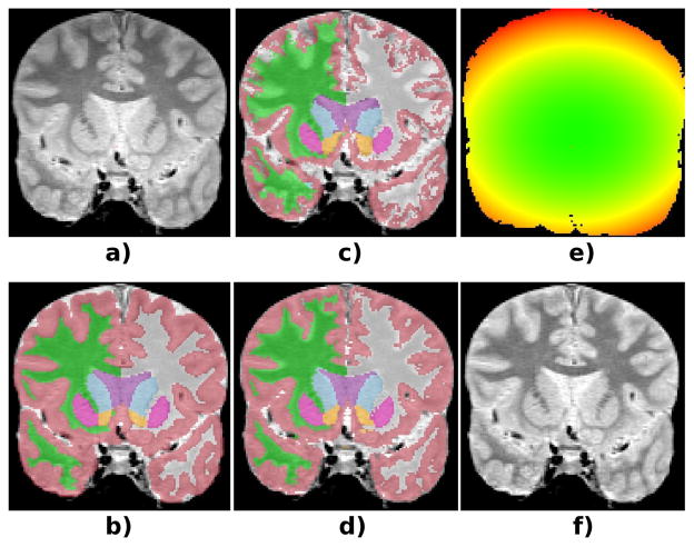
Figure 2 shows the Dice scores for the different methods and structures of interest, whereas Table 2 shows the averages across all structures. STAPLE and majority voting provide comparable results. The proposed method (for β = 0.75) significantly outperforms STAPLE for all brain structures except for the putamen. Compared with majority voting, the scores when β = 0.75 are significantly higher for WM, CT, LV, HP and CA, though not significantly different for TH, PU, PA and AM. The hippocampus, pallidum and especially the amygdala seem particularly difficult to segment in the PD-weighted dataset, since there is very little image contrast around them. When we compare the results from our method for β = 0 and β = 0.75, the difference is not large in absolute terms (approximately 0.6%), but it is statistically very significant; the higher β seems to fix some consistent mistakes that are made when the voxels are considered independently. Finally, Figure 3 shows a sample coronal slice of a target scan, illustrating the segmentations given by majority voting and the proposed method, as well as the estimated bias field.

Fig. 2.

Box plot of Dice scores for majority voting (black), STAPLE (red), β = 0 (green) and β = 0.75 (blue). The box has lines at the three quartile values. Whiskers extend to the most extreme values within 1.5 times the interquartile range from the ends of the box. Samples beyond those points are marked with circles. The purple S denotes that the scores are significantly lower than for our method at p=0.025.

Table 2.

Average Dice score across all structures for each method. The p-values correspond to a paired t-test which assesses whether the proposed method (at β = 0.75) produces a higher Dice score than each of the other algorithms.

Method	Maj.Vot.	STAPLE	β = 0	β = 0.75
Dice	0.766	0.762	0.796	0.802
p	2e-13	9e-22	3e-8	N/A

Fig. 3.

Coronal slice of a test subject. a) Original. b) Ground truth segmentation. c) Majority voting. d) Proposed method (β = 0.75). e) Bias field estimated by the proposed method (green=1.0, red=1.25). f) Bias-field corrected.

4. CONCLUSION

A method to perform inter-modality label fusion has been presented in this paper. The method exploits the intensities of the target image and, despite the low number of test subjects, achieves statistical significance when compared with majority voting and STAPLE in a challeging PD-weighted dataset. The MRF prior has a positive effect on the peformance of the method, significantly improving the Dice scores. We hypothesize that, as the number of available atlases grows, increasing β would be beneficial. As N → ∞, there would always be a training volume (almost) identical to the target case, and β = ∞ would provide a perfect segmentation.

The proposed inference method for the model can be improved by marginalizing over the labels when optimizing for the parameters, at the cost of introducing another level of complexity in the model. This will be addressed in future work, which will also include incorporating the registration in the optimization process, sweeping the parameters to assess their impact on segmentation accuracy, explicitly optimizing for ρ and testing the model on T₁ and multi-spectral data.

References

- 1.Collins DL, Holmes CJ, Peters TM, Evans AC. Automatic 3-d model-based neuroanatomical segmentation. Hum Brain Mapp. 1995;3:190–208. [Google Scholar]
- 2.Yeo BTT, Sabuncu MR, Desikan R, Fischl B, Golland P. Effects of registration regularization and atlas sharpness on segmentation accuracy. Med Image Anal. 2008;12(5):603–615. doi: 10.1016/j.media.2008.06.005. [DOI] [PMC free article] [PubMed] [Google Scholar]
- 3.Heckemann RA, Hajnal JV, Aljabar P, Rueckert D, Hammers A. Automatic anatomical brain mri segmentation combining label propagation and decision fusion. NeuroImage. 2006;33(1):115–126. doi: 10.1016/j.neuroimage.2006.05.061. [DOI] [PubMed] [Google Scholar]
- 4.Warfield SK, Zou KH, Wells WM. Simultaneous truth and performance level estimation (staple): an algorithm for the validation of image segmentation. IEEE Trans Med Im. 2004;23(7):903–921. doi: 10.1109/TMI.2004.828354. [DOI] [PMC free article] [PubMed] [Google Scholar]
- 5.Isgum I, Staring M, Rutten A, Prokop M, Viergever MA, van Ginneken B. Multi-atlas-based segmentation with local decision fusion: application to cardiac and aortic segmentation in ct scans. IEEE Trans Med Im. 2009;28(7):1000–1010. doi: 10.1109/TMI.2008.2011480. [DOI] [PubMed] [Google Scholar]
- 6.Sabuncu MR, Yeo BTT, Van Leemput K, Fischl B, Golland P. A generative model for image segmentation based on label fusion. IEEE Trans Med Im. 2010;29(10):1714–1729. doi: 10.1109/TMI.2010.2050897. [DOI] [PMC free article] [PubMed] [Google Scholar]
- 7.Ashburner J, Friston KJ. Unified segmentation. Neuroimage. 2005;26(3):839–851. doi: 10.1016/j.neuroimage.2005.02.018. [DOI] [PubMed] [Google Scholar]
- 8.Pohl K, Fisher J, Shenton M, McCarley R, Grimson W, Kikinis R, Wells W. Logarithm odds maps for shape representation. MICCAI. 2006:955–963. doi: 10.1007/11866763_117. [DOI] [PMC free article] [PubMed] [Google Scholar]
- 9.Caviness VS, Jr, Filipek PA, Kennedy DN. Magnetic resonance technology in human brain science: blueprint for a program based upon morphometry. Brain Dev. 1989;11(1):1–13. doi: 10.1016/s0387-7604(89)80002-6. [DOI] [PubMed] [Google Scholar]
- 10.Freesurfer wiki. http://surfer.nmr.mgh.harvard.edu.