Improving the Accuracy and Efficiency of Partitioning Heritability into the Contributions of Genomic Regions

Abstract

Quantifying heritability, the amount of genetic contribution in a complex trait, has been of fundamental interest to geneticists for decades. Recently, partitioning the heritability accounted for by common variants into the contributions of genomic regions has received a lot of attention given its important applications for understanding the genetic architecture of complex traits. Current methods partition the total heritability by jointly estimating the contributions of all regions. However, these methods are computationally intractable and can be inaccurate when the number of regions is large. In this paper, we present an alternative approach that partitions the total heritability into the contributions of an arbitrary number of regions. We demonstrate by using simulations that our approach is more accurate and computationally efficient than current approaches. Using a data set from a genome-wide association study on human height, we demonstrate the utility of our method by estimating the heritability contributions of chromosomes and subchromosomal regions.

Introduction

Quantifying heritability, the amount of genetic contribution in a complex trait, has been of fundamental interest to geneticists for decades.^1,2 Heritability, in the “narrow sense,”³ quantifies the influence of the additive genetics relative to the environment. Prior to the availability of genotyping technologies, heritabilities were estimated in studies of related individuals with known pedigrees, such as classical twin studies.⁴ These studies use a pedigree to infer the genetic relationship among the individuals; this relationship corresponds to the covariance structure among the individuals’ genetic effects. These studies are susceptible to confounding due to cryptic relatedness across families, which can lead to inaccurate heritability estimates.⁵

Recently developed genomic technologies have created new possibilities for estimating heritability.⁶ Information on millions of SNPs can be collected cost effectively from thousands of individuals. Using the realized genetic relationships inferred from the observed SNP data, a set of recently proposed methods have estimated the heritability of human height accounted for by common variants or rare variants in linkage disequilibrium (LD) with common variants.^7,8 These estimates using the common variants explain a large fraction of the total-heritability estimates obtained from twin studies.⁹ Furthermore, a recent genome-partitioning approach¹⁰ has estimated the heritability contributions of common variants in the autosomes by using the realized local genetic relationships among the individuals at each autosome.

Partitioning heritability into the contributions of genomic regions is a general problem with many applications, which include providing insights into the genetic architecture of a trait,¹⁰ quantifying the amount of population structure in a study cohort,^10,11 quantifying the effect of genes with a certain functional annotation in comparison to other genes,¹¹ quantifying the phenotypic variation explained by genic versus intergenic regions,¹⁰ and estimating the amount of corresponding variation within a previously identified quantitative-trait locus compared to the rest of the genome.¹² The current approach, implemented in the widely used method GCTA (Genome-wide Complex Trait Analysis),¹³ estimates the heritability contributions of all regions jointly. However, this approach becomes computationally intractable when the number of regions is large and the regions themselves are smaller than chromosomes.

In this paper, we present an alternative approach for estimating the contributions of an arbitrary number of regions to the total heritability. Using a linear mixed-model approach, we estimate the heritability contribution of each region separately. For each region, we partition the total heritability into the contribution of the region and its genomic complement and repeat this procedure for all regions similarly to the approach presented in Hayes et al.¹⁴ An advantage of our approach is that in addition to performing the computations in parallel, we also take advantage of spectral decomposition to efficiently estimate the variance components.^15,16 Overall, our approach is more efficient, especially when the number of regions increases.

Using simulations, we demonstrate that our proposed approach is more accurate than the current approach when the number of regions is over 100. In our simulations, we partition the genome into a large number of regions and consider different scenarios of heritability contributions from these regions. We further apply the proposed and current approaches to a data set from a large-scale genome-wide association study (GWAS) on human height.¹⁷ Both approaches estimate the same genome-wide heritability for height (62%) but estimate different heritability contributions from genomic regions. We also use our approach to estimate the proportion of the observed heritability accounted for as a result of population structure.

Material and Methods

GWAS Samples and Quality Control

We used the height measurements and the genotype data available from the Northern Finland Birth Cohort of 1966¹⁷ from 5,319 unrelated individuals who were phenotyped for height at 31 years of age. We adjusted the height measurements for sex. The data set contains 331,450 autosomal SNPs after application of the exclusion criteria of Hardy-Weinberg equilibrium (p < 10⁻⁴), genotyping completeness (<95%), and minor allele frequency (<1%).

Linear Mixed Model for Partitioning the Genome-wide Heritability

Using a linear mixed model, we attribute the phenotypic variation to additive-genetic effects and the environment,

$$\begin{array}{c}y=X{\beta }_f+\sum _{i\in \mathcal{G}}{\beta }_i{x}_i+e,\end{array}$$ (Equation 1)

where y is the n × 1 vector of the observed phenotypic values from n individuals, X is the n × p covariate matrix including the intercept, and ${\beta }_f$ is the p × 1 vector of the (unknown) fixed-effect parameters including the population mean. Let $\mathcal{G}$ denote the set of the observed SNPs across the genome. $x_i$, where $i\in \mathcal{G}$, denotes the n × 1 normalized genotype vector of SNP i with effect ${\beta }_i$, and the components of $x_i$ are encoded as $\{2-2p_i/\sqrt{2p_i\left(1-p_i\right)},1-2p_i/\sqrt{2p_i\left(1-p_i\right)},-2p_i/\sqrt{2p_i\left(1-p_i\right)}\}$ for minor allele homozygous, heterozygous, and major allele homozygous ($p_i$ is the observed minor allele frequency). We follow the standard approach and assume that the SNP effects are independent and normally distributed: ${\beta }_i\stackrel{\text{iid}}{\sim }\mathcal{N}\left(0,{\sigma }^2\right)$. Finally, e denotes the n × 1 vector of environmental effects in the trait; $e\sim \mathcal{N}\left(0,{\sigma }_e^{2}I\right)$, in which $I$ is the identity matrix. This model can be succinctly expressed as

$$\begin{array}{c}y=X{\beta }_f+g+e,\end{array}$$ (Equation 2)

where $g$ is the n × 1 vector of genetic effect such that $g\sim \mathcal{N}\left(0,{\sigma }^{2}K\right)$ and $K={\sum }_{i\in \mathcal{G}}{x}_i{x}_i^T$. The narrow-sense heritability accounted for by the genetic effect is defined and can be estimated as

$$\begin{array}{l}{h}_g^2=\frac{\text{Var}\left(g\right)}{\text{Var}\left(g+e\right)},\\ {\hat{h}}_g^2=\text{E}\left[h_g^2\right]\approx \frac{{\hat{\sigma }}^2\text{Tr}\left(PK\right)}{{\hat{\sigma }}^2\text{Tr}\left(PK\right)+n{\hat{\sigma }}_e^2},\end{array}$$ (Equation 3)

where $P=I-(1/n){11}^T$ and $\text{Tr}(·)$ denotes the matrix trace.

Given a genomic region defined by the set of SNPs $\mathcal{R}$, where $\mathcal{R}\subset \mathcal{G}$, we estimate the contribution of the region to the heritability by using the following model:

$$\begin{array}{c}y=X{\beta }_f+\sum _{r\in \mathcal{R}}{\beta }_r{x}_r+\sum _{b\in \mathcal{G}\setminus \mathcal{R}}{\beta }_b{x}_b+e,\end{array}$$ (Equation 4)

where ${\beta }_r\stackrel{\text{iid}}{\sim }\mathcal{N}\left(0,{\sigma }_r^2\right)$ and ${\beta }_b\stackrel{\text{iid}}{\sim }\mathcal{N}\left(0,{\sigma }_b^2\right)$. Equivalently,

$$\begin{array}{c}y=X{\beta }_f+r+b+e,\end{array}$$ (Equation 5)

where $r$ and $b$ are n × 1 vectors denoting the genetic effects of the region and its genomic background. Both genetic effects follow a multivariate normal distribution, $r\sim \mathcal{N}\left(0,{\sigma }_r^2{K}_r\right)$ and $b\sim \mathcal{N}\left(0,{\sigma }_b^2{K}_b\right)$, where $K_r={\sum }_{x_r\in \mathcal{R}}{x}_r{x}_r^T$ and $K_b={\sum }_{x_b\in \mathcal{G}\setminus \mathcal{R}}{x}_b{x}_b^T$ are the realized genetic relationship matrices (GRMs) among the individuals for the region and the genetic background calculated from SNP data, respectively. We note that inherent to our model is the assumption that $\text{Cov}\left(r,b\right)=0$, i.e., ${\sum }_{\forall x_r,\forall x_b}{x}_r\text{Cov}\left({\beta }_r,{\beta }_b\right)x_b^T=0$, given that $\text{Cov}\left({\beta }_r,{\beta }_b\right)=0$. We discuss this assumption in more detail in the Discussion. Finally, the phenotype vector follows a multivariate normal distribution,

$$\begin{array}{c}y\sim \mathcal{N}\left(X{\beta }_f,{\sigma }_r^2{K}_r+{\sigma }_b^2{K}_b+{\sigma }_e^{2}I\right).\end{array}$$ (Equation 6)

The total covariance due to additive genetics can be expressed as ${\sigma }_r^2{K}_r+{\sigma }_b^2{K}_b={\sigma }_g^2{K}_g$, where $K_g=\omega K_r+\left(1-\omega \right)K_b$. We determine the unknown variance scalars ${\sigma }_r^2=\omega {\sigma }_g^2$, ${\sigma }_b^2=\left(1-\omega \right){\sigma }_g^2$, and ${\sigma }_e^2$ by using the following approach that iterates over the parameter ω. For given ω, we transform the model to a coordinate system in which the covariance matrix ${\sigma }_g^2{K}_g+{\sigma }_e^{2}I$ is diagonal, which lets us find the maximum-likelihood parameters efficiently by speeding up the computationally expensive matrix inversion. We use the spectral transformation, $Q^T$, where $K_g=Q\Lambda Q^T$ is the eigendecomposition of the covariance structure of the genetic effect. The spectrally transformed model is

$$\begin{array}{c}\tilde{y}\sim \mathcal{N}\left(\tilde{X}{\beta }_f,{\sigma }_g^2\Lambda +{\sigma }_e^{2}I\right),\end{array}$$ (Equation 7)

where $\tilde{y}=Q^{T}y$ and $\tilde{X}=Q^{T}X$. We estimate the unknown variance parameters by using the restricted log-likelihood that takes into account the degrees-of-freedom loss that results from estimating the fixed-effect parameters,^18,19

$$\mathrm{ℒ}{\mathrm{ℒ}}_R\left({\sigma }_g^2,{\sigma }_e^2|\omega \right)=-\frac{1}{2}\left(\left(n-p\right)\log \left(2\pi \right)-\log \left(\left|{\tilde{X}}^T\tilde{X}\right|\right)+\log \left(\left|{\tilde{X}}^T{V}^{-1}\tilde{X}\right|\right)+\log \left(\left|V\right|\right)+{\left(\tilde{y}-\tilde{X}{\hat{\beta }}_f\right)}^T{V}^{-1}\left(\tilde{y}-\tilde{X}{\hat{\beta }}_f\right)\right),$$ (Equation 8)

where $V={\sigma }_g^2\Lambda +{\sigma }_e^{2}I$ and ${\hat{\beta }}_f={\left({\tilde{X}}^T{V}^{-1}\tilde{X}\right)}^{-1}{\tilde{X}}^T{V}^{-1}\tilde{y}$. In particular, the restricted log-likelihood can be expressed as an analytic function of $\delta ={\sigma }_e^2/{\sigma }_g^2$ and solved with Brent’s method for determining the global maximum likelihood.^15,16,20,21

Finally, the heritability contribution of the region is calculated as

$$\begin{array}{c}{\hat{h}}_r^2=\frac{{\hat{\sigma }}_r^2\text{Tr}\left(P{K}_r\right)}{{\hat{\sigma }}_g^2\text{Tr}\left(P{K}_g\right)+n{\hat{\sigma }}_e^2}.\end{array}$$ (Equation 9)

Normalization of the Heritability Contributions

One of the difficulties of partitioning the heritability into the contributions of genomic regions is the LD structure of the genome. When HEIDI (Heritability Estimations Distributed) estimates the heritability contribution of a region, the background model can inadvertently capture a portion of the heritability as a result of the inclusion of markers in the background GRM (these markers are in LD with markers in the region).

We utilize the following normalization procedure to improve the accuracy of the estimates obtained from HEIDI, which mitigates the effect of LD. First, we estimate the total heritability and subsequently estimate the contributions of the autosomes and scale their contributions such that their sum equals the total heritability. The advantage of these estimates is that they are not affected by LD. We then estimate the heritability contributions of the regions and normalize the regions’ contributions in each chromosome such that their sum equals the normalized chromosomal contribution.

Simulation Model

In our simulations, we partitioned each of the 22 autosomes into five regions of equal numbers of SNPs and used the following model to generate phenotype values:

$$\begin{array}{c}y=1\mu +\sum _{i=1}^{110}{r}_i+e,\end{array}$$ (Equation 10)

where $r_i\sim \mathcal{N}\left(0,{\sigma }_i^2{K}_i\right)$and $i\in \left\{1,\dots ,110\right\}$ are the variance components, each with the covariance matrix $K_i$, accounting for the chromosome regions, and $e\sim \mathcal{N}\left(0,{\sigma }_e^{2}I\right)$ is the error term. The total heritability and the contributions of the regions in the total heritability are determined by the selection of variance scalars, ${\sigma }_i^2$’s and ${\sigma }_e^2$, accordingly. Finally, phenotype values are generated via sampling from the corresponding multivariate normal distribution,

$$y_{\text{sim}}\sim \mathcal{N}\left(1\mu ,\sum _{i=1}^{110}{\sigma }_i^2{K}_i+{\sigma }_e^{2}I\right).$$ (Equation 11)

Results

HEIDI Is More Accurate Than the Current Approach

We compare HEIDI to the widely used method, GCTA,¹³ which partitions the heritability into the contributions of genomic regions. Using a linear mixed model, GCTA assigns a variance component to each region and jointly estimates their heritability contributions.

Our approach estimates these contributions separately for each region in two stages. First, we partition the phenotypic variation to that attributable to the total additive genetic effect of the whole genome and the environment. This allows us to estimate the genome-wide heritability, as well as predict the total genetic effect. Next, we estimate the heritability contribution of a region by breaking the total genetic effect into the effects of the region and the rest of the genome. This step is repeated for each region separately and can be performed in parallel for improving the computational efficiency. Finally, the contributions of the chromosomes are normalized to that of the total heritability, and the contributions of regions in each chromosome are normalized to that of the whole chromosome.

We performed simulations by using the genotype data available from the Northern Finland Birth Cohort.¹⁷ The data consist of 331,450 common SNPs that passed various exclusion criteria on 5,319 unrelated individuals (see Material and Methods). We partitioned each of the 22 autosomes into five regions, which each contained an equal number of SNPs. We utilized the same number of markers per region to minimize any possible bias that might result from using a different number of markers for computing the GRMs in each chromosome. We used the same approach as in the GCTA software to estimate the GRMs. For our simulations, we generated phenotypes by sampling from a multivariate normal distribution with a covariance matrix, which is the environmental noise plus the sum of the GRMs weighted by their region contributions in the heritability. We generated three panels of simulations, each with 100 replicates. In these simulations, we set the genome-wide heritability to 50%.

In the first panel, each region had the same heritability contribution. In the second panel, chromosomes contributed to the heritability proportionally to their sizes; the contributions of each chromosome ranged from 6.96%–0.32% of the total heritability, and the contributions of the five regions in each chromosome ranged from 32%–8% of the chromosome’s contribution itself. In this scenario, there was a wide range of heritabilities for different regions. In the third panel, we simulated a scenario in which chromosomal regions 2 and 4 did not contribute to the heritability but in which regions 1, 3, and 5 had equal contributions.

We compared the accuracy of the two methods across the simulations with respect to their mean absolute error (MAE). In a region, the absolute error is the magnitude of the difference between the estimated heritability contribution of the region and its true value. In each method, we obtained the absolute errors of the regions in each simulation replicate. The MAE per region is the average of the absolute errors over the replicates. Note that the unit of MAE is heritability. In the first simulation panel, in which the regions had the same contribution, the MAE values were 0.33 for HEIDI and 0.37 for GCTA. In the second panel, in which the contributions changed with chromosome size, the MAE values were 0.32 for HEIDI and 0.34 for GCTA. In the third panel, in which the contributions were sparse, the MAE values were 0.32 for HEIDI and 0.34 for GCTA. Our results suggest that, on average, HEIDI is over 5% more accurate than GCTA in partitioning the total heritability. Figures 1–3 show the MAE of each method in each region. In terms of computation, HEIDI can estimate the contribution of each region in parallel, which significantly facilitates estimating the heritability contributions of many regions.

Figure 1.

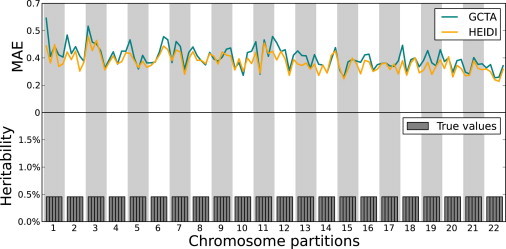
Simulations Using Uniform Heritability Contributions

MAE values obtained by HEIDI and GCTA are shown in each region in the simulations where the total heritability is 50% and each region has the same heritability contribution. In this scenario, the accuracy of HEIDI is 8.76% higher than that of GCTA.

Figure 2.

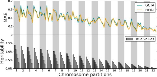
Simulations Using Varying Heritability Contributions

MAE values obtained by HEIDI and GCTA are shown in each region in the simulations where the total heritability is 50% and the regions have heritability contributions that vary across the genome. In this scenario, the accuracy of HEIDI is 3.64% higher than that of GCTA.

Figure 3.

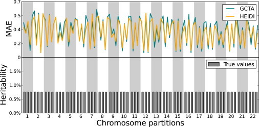
Simulations Using Sparse Heritability Contributions

MAE values obtained by HEIDI and GCTA are shown in each region in the simulations where the total heritability is 50% and in each chromosome, the second and fourth regions do not contribute to the heritability, and the first, third, and fifth regions have equal contributions. In this scenario, the accuracy of HEIDI is 3.36% higher than that of GCTA.

Partitioning the Heritability of Human Height and Estimating the Contribution of Population Structure

We applied both approaches to the height phenotype collected from the Northern Finland Birth Cohort GWAS data.¹⁷ We estimated the total heritability, the contributions of the autosomes, and their partitions accounted for by common variants in the genome. We used the same approach to estimate the GRMs as in the GCTA software.

For the unpartitioned genome, both approaches estimated 62.4% heritability, which is expected given that they use the same underlying model. We partitioned the genome-wide heritability into the contributions of the 22 autosomes, shown in Figure 4. Both methods estimated similar contributions with high concordance. However, when heritability was partitioned into contributions from smaller regions, differences between GCTA and HEIDI emerged. In Figure 5, the heritability contributions of each autosome are split into five regions of equal numbers of SNPs.

Figure 4.

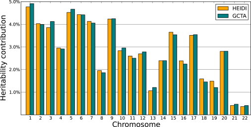
Partitioning the Heritability of Height into Chromosomes

HEIDI- and GCTA-estimated heritability contributions of the 22 autosomal chromosomes to height are shown.

Figure 5.

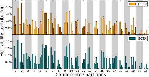
Partitioning the Heritability of Height into Chromosomal Regions

The heritability of height is partitioned into the contributions of chromosomal regions. For many regions, GCTA estimates no heritability contribution.

One of the main applications of partitioning the heritability into contributions from genomic regions is that it allows us to estimate the contribution of population structure to the observed heritability. Both population structure and cryptic relatedness are known to increase estimates of heritability.^10,22 We compared HEIDI and GCTA in performing the analysis described in Yang et al.,¹⁰ where they partitioned the heritability into chromosomes and compared these estimates to those of the heritability by using only one variance component corresponding to the GRM from the chromosome. The idea is that in the presence of population structure or cryptic relatedness, an estimate from a single chromosome will capture part of the heritability from the rest of the genome. The lengths of the regions are then regressed on the difference between these estimates, as shown in Figure 6. Yang et al.¹⁰ interpreted the intercept as corresponding to a measure of the cryptic relatedness and the slope as corresponding to a measure of the population structure. The reasoning behind the hypothesized linear relationship between the length of the region and the difference in heritability estimates is due to the number of ancestral informative markers present in a region; this number of informative markers is in turn proportional to the length of the region if one assumes that the markers are evenly spaced. HEIDI estimates the slope and intercept of the graph at 7.51 × 10⁻⁵ and 0.0116, respectively, whereas GCTA estimates the slope and intercept at 6.84 × 10⁻⁵ and 0.0124, respectively. According to the approach described in Yang et al.,¹⁰ these correspond to estimates of the population-structure contributions to heritability of 0.99% for HEIDI and 0.91% for GCTA. We can compare the performance of HEIDI to that of GCTA in these estimates by considering how well the regression line fits the data in Figure 6 by measuring the residual sum of squares (RSS). Intuitively, the better the fit, the better the method captures the population-structure signal from ancestry-informative markers. With an RSS of 5.30 × 10⁻⁴, HEIDI outperforms GCTA, which has an RSS of 5.54 × 10⁻⁴.

Figure 6.

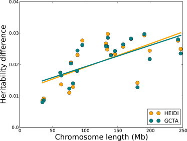
Regression of Differences in Heritability Estimates on Chromosome Length

The difference between the heritability contributions of each chromosome is estimated from heritability partitioning and estimated independently of the rest of the genome; it is regressed against the length of the chromosome.

We also estimated the contribution of population structure by using regions smaller than chromosomes, and the corresponding regression is shown in Figure S1. Although the formula for estimating the population-structure contributions in Yang et al.¹⁰ does not immediately apply to estimates from shorter regions, the heritability estimates of HEIDI (RSS = 1.03 × 10⁻³) fit the linear model better than those of GCTA (RSS = 1.12 × 10⁻³).

Discussion

A fundamental part of genetics is to understand the influence of genetic variation in complex traits. In tackling this task, traditional studies have used related individuals to estimate the influence of genetics relative to the environment. Recently, there has been growing interest in estimating heritabilities from GWAS data sets containing large numbers of unrelated individuals. The total heritability can be partitioned into the contributions of the autosomes by the inclusion of a variance component representing the contribution of each autosome and the joint estimation of their contributions to the trait, as implemented in the widely used method GCTA. However, as the number of regions increase and the regions themselves become smaller, this approach becomes computationally intractable. We propose HEIDI, an alternative method that partitions the heritability into the contributions of an arbitrary number of regions. For each region, HEIDI decomposes the heritability as the sum of the contribution of the region and the contribution of the remainder of the genome. Finally, the heritability contributions are normalized such that their sum equals the genome-wide heritability. Using simulations, we compared the performance of HEIDI to that of GCTA. On average, HEIDI performed over 5% more accurately than GCTA when estimating heritability contributions and could estimate these contributions in parallel.

One explanation for the improved accuracy of our approach is that the search space of the partitioned heritability has over 100 dimensions when we consider five regions per chromosome and that this space contains many local maxima. Whereas GCTA searches the entire space, our approach takes advantage of spectral decomposition to find the maximum-likelihood solutions in a restricted version of the space. Even though the maximum in the space searched by GCTA is higher than HEIDI’s, the fact that HEIDI finds the maximum likelihood of the restricted space efficiently might end up being a better solution than GCTA’s. We compared GCTA to HEIDI when partitioning the heritability into only two regions, and as expected, the two methods found very similar estimates; this is consistent with our explanation because the search space when only two regions are considered is relatively small.

Consistent with current approaches to estimating heritability from unrelated individuals, our approach assumes an additive-genetic model, in which the covariance between any two regions, and by extension any region and its corresponding genomic background, is zero. The presence of gene-gene interactions, or epistatis, will violate this assumption and cause inaccuracies in our estimates of regional heritability contributions similarly to how they affect total heritability estimates.^23,24 In addition, LD between markers in neighboring regions will cause this assumption to be violated and cause the estimate of the heritability contribution of a region to be spread among the region along with the neighboring regions. However, this phenomenon is equivalent to how a causal variant causes neighboring variants in LD to also have elevated statistics in a GWAS and is inherent because of the LD structure of the human genome. HEIDI’s normalization of the region contribution estimates mitigates the effect of LD on the estimates.

Gene-gene interactions are not the only reason for observing deviations from the additive model. The presence of population structure in the sample might lead to inflation of the estimates of heritability of each region when they are estimated individually and cause the sum of the estimates from the regions to differ from the estimate of the total heritability.^8,10 HEIDI reports both the normalized estimates of heritability and the unnormalized estimates and can also be used to estimate the contribution of each region independently by omitting the background model. The differences between these estimates provide evidence of deviation from an additive model, which can be explained by population structure or interaction effects.

Web Resources

The URL for data presented herein is as follows:

• HEIDI, http://genetics.cs.ucla.edu/heritability/

References

- 1.Fisher R.A. The correlation between relatives on the supposition of Mendelian inheritance. Philosophical Transactions of the Royal Society of Edinburgh. 1918;52:399–433. [Google Scholar]
- 2.Falconer D.S., Mackay T.F.C. Benjamin Cummings; New York: 1996. Introduction to Quantitative Genetics. [Google Scholar]
- 3.Visscher P.M., Hill W.G., Wray N.R. Heritability in the genomics era—concepts and misconceptions. Nat. Rev. Genet. 2008;9:255–266. doi: 10.1038/nrg2322. [DOI] [PubMed] [Google Scholar]
- 4.van Dongen J., Slagboom P.E., Draisma H.H.M., Martin N.G., Boomsma D.I. The continuing value of twin studies in the omics era. Nat. Rev. Genet. 2012;13:640–653. doi: 10.1038/nrg3243. [DOI] [PubMed] [Google Scholar]
- 5.Sham P.C., Cherny S.S., Purcell S. Application of genome-wide SNP data for uncovering pairwise relationships and quantitative trait loci. Genetica. 2009;136:237–243. doi: 10.1007/s10709-008-9349-4. [DOI] [PubMed] [Google Scholar]
- 6.Zaitlen N., Kraft P. Heritability in the genome-wide association era. Hum. Genet. 2012;131:1655–1664. doi: 10.1007/s00439-012-1199-6. [DOI] [PMC free article] [PubMed] [Google Scholar]
- 7.Kang H.M., Sul J.H., Service S.K., Zaitlen N.A., Kong S.Y., Freimer N.B., Sabatti C., Eskin E. Variance component model to account for sample structure in genome-wide association studies. Nat. Genet. 2010;42:348–354. doi: 10.1038/ng.548. [DOI] [PMC free article] [PubMed] [Google Scholar]
- 8.Yang J., Benyamin B., McEvoy B.P., Gordon S., Henders A.K., Nyholt D.R., Madden P.A., Heath A.C., Martin N.G., Montgomery G.W. Common SNPs explain a large proportion of the heritability for human height. Nat. Genet. 2010;42:565–569. doi: 10.1038/ng.608. [DOI] [PMC free article] [PubMed] [Google Scholar]
- 9.Silventoinen K., Sammalisto S., Perola M., Boomsma D.I., Cornes B.K., Davis C., Dunkel L., De Lange M., Harris J.R., Hjelmborg J.V.B. Heritability of adult body height: a comparative study of twin cohorts in eight countries. Twin Res. 2003;6:399–408. doi: 10.1375/136905203770326402. [DOI] [PubMed] [Google Scholar]
- 10.Yang J., Manolio T.A., Pasquale L.R., Boerwinkle E., Caporaso N., Cunningham J.M., de Andrade M., Feenstra B., Feingold E., Hayes M.G. Genome partitioning of genetic variation for complex traits using common SNPs. Nat. Genet. 2011;43:519–525. doi: 10.1038/ng.823. [DOI] [PMC free article] [PubMed] [Google Scholar]
- 11.Lee S.H., DeCandia T.R., Ripke S., Yang J., Sullivan P.F., Goddard M.E., Keller M.C., Visscher P.M., Wray N.R., Schizophrenia Psychiatric Genome-Wide Association Study Consortium (PGC-SCZ) International Schizophrenia Consortium (ISC) Molecular Genetics of Schizophrenia Collaboration (MGS) Estimating the proportion of variation in susceptibility to schizophrenia captured by common SNPs. Nat. Genet. 2012;44:247–250. doi: 10.1038/ng.1108. [DOI] [PMC free article] [PubMed] [Google Scholar]
- 12.Signer-Hasler H., Flury C., Haase B., Burger D., Simianer H., Leeb T., Rieder S. A genome-wide association study reveals loci influencing height and other conformation traits in horses. PLoS ONE. 2012;7:e37282. doi: 10.1371/journal.pone.0037282. [DOI] [PMC free article] [PubMed] [Google Scholar]
- 13.Yang J., Lee S.H., Goddard M.E., Visscher P.M. GCTA: a tool for genome-wide complex trait analysis. Am. J. Hum. Genet. 2011;88:76–82. doi: 10.1016/j.ajhg.2010.11.011. [DOI] [PMC free article] [PubMed] [Google Scholar]
- 14.Hayes B.J., Pryce J., Chamberlain A.J., Bowman P.J., Goddard M.E. Genetic architecture of complex traits and accuracy of genomic prediction: coat colour, milk-fat percentage, and type in Holstein cattle as contrasting model traits. PLoS Genet. 2010;6:e1001139. doi: 10.1371/journal.pgen.1001139. [DOI] [PMC free article] [PubMed] [Google Scholar]
- 15.Patterson H.D., Thompson R. Recovery of inter-block information when block sizes are unequal. Biometrika. 1971;58:545–554. [Google Scholar]
- 16.Kang H.M., Zaitlen N.A., Wade C.M., Kirby A., Heckerman D., Daly M.J., Eskin E. Efficient control of population structure in model organism association mapping. Genetics. 2008;178:1709–1723. doi: 10.1534/genetics.107.080101. [DOI] [PMC free article] [PubMed] [Google Scholar]
- 17.Sabatti C., Service S.K., Hartikainen A.-L., Pouta A., Ripatti S., Brodsky J., Jones C.G., Zaitlen N.A., Varilo T., Kaakinen M. Genome-wide association analysis of metabolic traits in a birth cohort from a founder population. Nat. Genet. 2009;41:35–46. doi: 10.1038/ng.271. [DOI] [PMC free article] [PubMed] [Google Scholar]
- 18.Harville D.A. Bayesian inference for variance components using only error contrasts. Biometrika. 1974;61:383–385. [Google Scholar]
- 19.Harville D.A. Maximum likelihood approaches to variance component estimation and to related problems. J. Am. Stat. Assoc. 1977;72:320–338. [Google Scholar]
- 20.Lynch M., Walsh B. Sinauer Associates; Sunderland, MA: 1998. Genetics and Analysis of Quantitative Traits. [Google Scholar]
- 21.Lippert C., Listgarten J., Liu Y., Kadie C.M., Davidson R.I., Heckerman D. FaST linear mixed models for genome-wide association studies. Nat. Methods. 2011;8:833–835. doi: 10.1038/nmeth.1681. [DOI] [PubMed] [Google Scholar]
- 22.Browning S.R., Browning B.L. Population structure can inflate SNP-based heritability estimates. Am. J. Hum. Genet. 2011;89:191–193. doi: 10.1016/j.ajhg.2011.05.025. author reply 193–195. [DOI] [PMC free article] [PubMed] [Google Scholar]
- 23.Zuk O., Hechter E., Sunyaev S.R., Lander E.S. The mystery of missing heritability: Genetic interactions create phantom heritability. Proc. Natl. Acad. Sci. USA. 2012;109:1193–1198. doi: 10.1073/pnas.1119675109. [DOI] [PMC free article] [PubMed] [Google Scholar]
- 24.Bloom J.S., Ehrenreich I.M., Loo W.T., Lite T.L., Kruglyak L. Finding the sources of missing heritability in a yeast cross. Nature. 2013;494:234–237. doi: 10.1038/nature11867. [DOI] [PMC free article] [PubMed] [Google Scholar]
Associated Data
This section collects any data citations, data availability statements, or supplementary materials included in this article.