Segmentation of lung lesions on CT scans using watershed, active contours, and Markov random field

Abstract

Purpose: Lung lesions vary considerably in size, density, and shape, and can attach to surrounding anatomic structures such as chest wall or mediastinum. Automatic segmentation of the lesions poses a challenge. This work communicates a new three-dimensional algorithm for the segmentation of a wide variety of lesions, ranging from tumors found in patients with advanced lung cancer to small nodules detected in lung cancer screening programs.

Methods: The authors’ algorithm uniquely combines the image processing techniques of marker-controlled watershed, geometric active contours as well as Markov random field (MRF). The user of the algorithm manually selects a region of interest encompassing the lesion on a single slice and then the watershed method generates an initial surface of the lesion in three dimensions, which is refined by the active geometric contours. MRF improves the segmentation of ground glass opacity portions of part-solid lesions. The algorithm was tested on an anthropomorphic thorax phantom dataset and two publicly accessible clinical lung datasets. These clinical studies included a same-day repeat CT (prewalk and postwalk scans were performed within 15 min) dataset containing 32 lung lesions with one radiologist's delineated contours, and the first release of the Lung Image Database Consortium (LIDC) dataset containing 23 lung nodules with 6 radiologists’ delineated contours. The phantom dataset contained 22 phantom nodules of known volumes that were inserted in a phantom thorax.

Results: For the prewalk scans of the same-day repeat CT dataset and the LIDC dataset, the mean overlap ratios of lesion volumes generated by the computer algorithm and the radiologist(s) were 69% and 65%, respectively. For the two repeat CT scans, the intra-class correlation coefficient (ICC) was 0.998, indicating high reliability of the algorithm. The mean relative difference was −3% for the phantom dataset.

Conclusions: The performance of this new segmentation algorithm in delineating tumor contour and measuring tumor size illustrates its potential clinical value for assisting in noninvasive diagnosis of pulmonary nodules, therapy response assessment, and radiation treatment planning.

INTRODUCTION

Despite improvements in staging, surgery, radiotherapy, and chemotherapy in the past three decades, lung cancer is still the leading cause of cancer-related death in the United States. The overall 5-yr survival rate remains about 13%.¹ Newer generation targeted therapies have begun to demonstrate clinical promise in lung cancer. However, many of these agents are cytostatic and do not cause rapid tumor shrinkage, or may cause less lesion shrinkage than previous generations of cytotoxic chemotherapy. Such difference in response patterns in successfully treated tumors is challenging to the traditional response assessment metrics which are based on measuring tumor diameters on CT or MR examinations.² These metrics primarily use linear or unidimensional measurements which do not adequately capture changes in tumor burden, especially when tumor changes are small and/or asymmetric. A recent study showed that early change in tumor volume is more sensitive than early diameter change at predicting EGFR mutation in nonsmall cell lung cancer following gefitnib therapy.³ The potential role volumetric CT may play in more timely and accurate therapy response assessment is currently under intensive investigation.⁴

To efficiently and reliably obtain tumor volumes on CT or MRI, computer aided techniques are essential. There are a number of algorithms published for the segmentation of small pulmonary nodules (usually less than 2 cm in diameter) on CT images.^{5, 6, 7, 8, 9, 10} In fact, the majority of segmentation algorithms developed so far aim at quantifying change in small lung nodules detected in CT lung cancer screening programs; where they were validated either visually or using a dataset containing small lung nodules, including a subset of the Lung Image Database Consortium (LIDC) database populated mainly with small nodules.¹¹ Such algorithms may not work up to par when applied to larger lung cancer tumors that are, for example, attached to surrounding structures of lesion density. Zhao et al. proposed to use multicriteria, including density and morphology, to segment and follow-up small pulmonary nodules.^{5, 6, 7} By varying threshold values over a specific density range, the algorithms automatically determined an optimal threshold that best separated a nodule from its surroundings based on surface gradient strength of the nodule candidates detected at different thresholds. Vessels could be removed by a shape constraint using the morphological operator with an automatically determined filter size. The algorithm was later modified for semiautomated segmentation of lung cancer tumors for therapy response assessment,¹² and several similar approaches were subsequently published.^{8, 9, 10} Threshold-morphology based methods have their limitations in segmenting nodules of irregular shapes or nodules that share a large portion of their surface with a surrounding structure (e.g., chest wall, mediastinum) of similar density.

Dehmeshki et al. proposed to use sphericity and contrast-based region-growing on a fuzzy map generated by relative fuzzy connectedness.¹³ The fuzzy map was used to improve the contrast between nodules and surrounding structures, such as blood vessels. The authors provided a subjective evaluation of their algorithm. Wang et al. proposed a method that transformed a nodule volume of interest (VOI) into a 2D image by using a spiral-scanning technique.¹⁴ Nodule boundary was detected on the 2D image by dynamic programming and then transformed back to 3D. Density drops along the radial lines were taken into consideration in the cost function. This method may not be valid for complex lung lesions as it assumes that each scan line intersects the lesion only once and that the nodule is brighter than its background.

Active contours have attracted great attention in the image segmentation research community since the seminal work of Kass et al.¹⁵ Way et al. proposed an explicit active contour method which minimized an energy that took into account 3D gradient, curvature, and penalized contours when growing against chest wall.¹⁶ However, the explicit active contour method is sensitive to initial condition and difficult to reposition the points on the 3D surface periodically.

This work presents a novel method for efficient and accurate lung lesion segmentation. Our approach is to use an edge-based method for solid lesions and a probability-based method for the ground glass opacity (GGO) portion of a lesion. GGO represents an increase of the attenuation of the lung without obscuring the bronchial and vascular margins. We used marker controlled watershed^{17, 18} to obtain an initial surface that was often close to the lesion boundary. We then deformed the initial lesion boundary using an active contour technique to smooth the initial surface while preserving its details. If the lesion was estimated to be part-solid, the GGO region was segmented by Markov random field (MRF). We will describe the segmentation method in detail in Sec. 2, demonstrate segmentation results in Sec. 3, and conclude the paper with discussions in Secs. 4, 5.

METHODS AND MATERIALS

The workflow of the algorithm was illustrated in Fig. 1. After manually selecting an elliptical region-of-interest (ROI) that enclosed a lesion on one slice (the reference slice), a VOI was created and resampled, and the elliptical ROI was extended to an elliptical cylinder. The location and size of the lesion on the reference slice was estimated, based on which the lesion marker (internal marker) was determined, and the tumor was estimated to be solid or part-solid. The region outside the elliptical cylinder and regions with the density of lung parenchyma served as the external markers. Using these markers and suppressing the strength of gradients closer to the center of the lesion, an initial segmentation result was obtained by marker-controlled watershed transform. An active contour model was applied to refine the lesion boundary. For part-solid or GGO lesions, the GGO portion was segmented by MRF and combined with the first segmentation result, followed by morphological opening operations to yield the final segmentation.

Figure 1.

Flowchart of the algorithm.

Initial segmentation by watershed segmentation

Determination of lesion VOI

The algorithm required the user to identify an elliptical ROI on one axial slice (reference slice) of the image series containing the lesion, which involved only a click, drag, and release of the mouse. The click defined the center of the ellipse and the distance between the releasing point and the center point in x and y direction indicated the semimajor and semiminor axis. Letting the elliptical ROI that encloses the lesion [Fig. 2a] center at O_o with semimajor axis a and semiminor axis b, the lesion VOI was defined as a rectangular prism that covers the ellipse in the X-Y plane and the slices within (a + b) × pixel spacing distance from the reference slice along the Z-axis in both directions. The VOI was then isotropically resampled to the in-plane resolution. The subsequent image processing techniques were performed on the resampled VOI.

Figure 2.

Segmentation of a lesion. (a) A lesion with manually drawn ROI, (b) result of applying threshold operation, (c) result after morphological operation and filling holes, (d) map resulted from the distance transformation, the center being the point with maximum distance in the image, (e) estimated lesion size (circle), the “+” indicating the recalculated center O and the length of the radial line indicating R hat, (f) watershed segmentation result with irregular boundary and vessels, and (g) active contour evolution result with the boundary smoothed and vessels detached.

Determination of markers

The marker-controlled watershed divides the image into disjoint regions by identifying watershed lines between adjacent markers.^{17, 18} In our application, the markers were one lesion marker (internal marker) and one or more background markers (external markers). We determined the internal marker by finding a threshold and using distance transform on the reference slice; the external marker(s) was determined from the surrounding parenchyma and the region outside the elliptical cylinder of the VOI.

To determine a threshold that separated the lesion from parenchyma, a Gaussian mixture model was employed. Since the ROI contains both lesion and lung parenchyma pixels, density distribution of the pixels could be modeled by two Gaussian distributions: P(x|nodule) and P(x|paren), where x was the pixel density and paren denoted parenchyma. The mean values and variations of the two Gaussian distributions were then estimated by the expectation-maximization method. The proportions of object P(nodule) and background P(paren) were also estimated. According to the Bayesian decision theory, a pixel with density x could be classified as a lesion pixel if the a posteriori probability P(nodule|x) was greater than P(paren|x), i.e., the threshold T was taken as the x, where

$$P\left(x\right|\mathrm{nodule}\left)P\right(\mathrm{nodule})=P(x\left|\mathrm{paren}\right)P\left(\mathrm{paren}\right).$$ (1)

Figure 3 shows the histogram of a lesion ROI on the reference slice. Two estimated Gaussian distributions were overlaid on the histogram, as was the threshold determined by Eq. 1.

Figure 3.

Threshold estimation for separating lesion from lung parenchyma in the ROI of Fig. 2a. The Gaussian curve to the left representing the density distribution of the lung parenchyma and the Gaussian curve to the right representing that of the lesion.

The regions of higher density than the threshold were considered to be candidates of the lesion [Fig. 2b]. The binary image was morphologically opened then closed to remove noise. The largest object was extracted and holes were filled [Fig. 2c]. To make the algorithm less sensitive to the user-specified center of the ROI, a new center O was calculated. A distance transform was applied to calculate the distance of each object pixel to its nearest background pixel [Fig. 2d].¹⁹ The pixel O that had the local maximum value on the distance image can be found by walking from O_o to its neighbors with the largest distance value until a local maximum was reached. The maximum distance $\widehat{R}$ corresponded to the radius of the maximum inscribed circle centered at the point O. A circle that was centered at O with a radius $\widehat{R}$ was taken as the estimated size of the lesion [Fig. 2e].

The nodules were classified into two types: solid and nonsolid (part-solid or pure GGO). The two types could be differentiated by their densities. If the mean density of the regions above the threshold T, the x that satisfied Eq. 1, was low (less than −150 HU, which is lower than the density of fat and higher than the mean density of GGO), the nodule was considered part-solid; otherwise it was considered solid. For part-solid nodules an extra step, i.e., a MRF model, was employed to segment the GGO portion.

Although the watershed surface was often located at strong continuous edges, it could be attracted by spurious edges far from the lesion boundary if a path with a small gradient connected the object and the background markers. The object marker should preferably be in proximity to the background markers.

The object marker was chosen as a circle, centered at O, with a radius of half of $\widehat{R}$. The ellipse ROI was applied to each slice of the VOI; pixels outside the ellipse were considered background markers. Large regions with densities of typical lung parenchyma (less than −870 HU) or high density regions such as vessels on contrast enhanced scan (greater than 200 HU) were also considered background markers.

Marker controlled watershed segmentation

The watershed transform was applied to a modified gradient image of the VOI. The gradient image was obtained by Sobel operators. In an ideal situation the lesion boundary would be the only edge in the image, but in reality there were often other edges between internal and external markers. To achieve a better result, the strength of those edges could be suppressed by multiplying the gradient image by a bowl-shaped function f(r):

$$f\left(r\right)=\left\{\begin{array}{cc}\hfill {\left(\frac{r}{\widehat{R}}\right)}^2& \hfill \mathrm{if}r<\widehat{R}\\ \hfill 1& \hfill \mathrm{if}r\ge \widehat{R}\end{array}\right.,$$ (2)

where r was the distance of each voxel to the center O. The function was less than 1 inside the ball of the radius $\widehat{R}$ and equal to 1 outside the ball. Inside the ball, the function was proportional to the square of the radius from the center. Applying the edge suppression served to lower the catchment basin for the lesion, so that the watershed method could potentially work better.

The markers were made the only local minimums by morphological reconstruction.¹⁸ A watershed surface was obtained by applying watershed transformation to the reconstructed image. Figure 2f shows a slice of the watershed surface. Though the surface was often close to the lesion boundary, parts of the surrounding structure, such as vessels, may have been segmented as the lesion. In order to refine the surface, a morphological opening operation was carried out with a spherical structural element, the radius of which was selected as 30% of the radius of the maximum inscribed sphere in the watershed surface. The radius was chosen by trial and error; it was adaptive to lesion size and it was a trade-off between detaching nonlesion structures and preserving boundary details. The largest connected component was taken as an initial segmentation of the lesion. The morphological operation could remove some undesired anatomical structures that attach to a lesion, but it could also remove the surface detail of the lesion. An implicit active contour method was employed to evolve the surface to the desired boundary while keeping the surface smooth.

Refinement

Refinement by active contours

Our model was based on the geometric snake model.^{20, 21} In level set representation, the model deforms an initial curve to minimize the weighted length (surface area) of its boundary:

$$\varepsilon \left(\varphi \right)=\int g\delta \left(\varphi \right)\left|\nabla \varphi \right|dxdydz,$$ (3)

where ϕ is the level set representation of the curve and g is an edge detection function, which is a positive and decreasing function of the gradient that has the form

$$g=\frac{1}{1+{\left(\nabla G_{\sigma }*I\right)}^2},$$ (4)

where I is the image and G_σ is a Gaussian Kernel with standard deviation σ. Minimizing ɛ(ϕ) results in the following gradient flow according to the Euler-Lagrange equation:

$${\varphi }_t=g\delta \left(\varphi \right)\kappa +\nabla g·\nabla \varphi \frac{\delta \left(\varphi \right)}{\left|\nabla \varphi \right|},$$ (5)

where δ is the Dirac delta function and κ is the local mean curvature defined as $\kappa =div\left(\frac{\nabla \varphi }{\left|\nabla \varphi \right|}\right)$. δ(ϕ) can be replaced by |∇ϕ| according to Zhao et al.;²² therefore we have

$${\varphi }_t=g\kappa \left|\nabla \varphi \right|+\nabla g·\nabla \varphi .$$ (6)

The first term is a mean curvature flow weighted by the edge detection function. The second term acts as a potential well, which drags the surface back when it crosses the object boundary. From our observation, the potential well was sometimes not deep enough to prevent the surface from passing through the boundary. We strengthened the potential well by increasing its coefficient term α as seen in the following equation:

$${\varphi }_t=g\kappa \left|\nabla \varphi \right|+\alpha \nabla g·\nabla \varphi .$$ (7)

To regulate the shape of the contour, we employed a volume preserving mean curvature flow technique.²³ The mean curvature flow is the evolution of a curve by ϕ_t = κ|∇ϕ|, which is the fastest way to minimize the perimeter (surface area) of an object. By subtracting the mean curvature as in the following equation,

$${\varphi }_t=\left(\kappa -{\kappa }_{\mathrm{mean}}\right)\left|\nabla \varphi \right|,$$ (8)

which will evolve a contour to a round one while preserving the volume. When the curve is a circle, the right term in the above equation is zero and the curve will stop evolving.

With a weighted potential well and volume preserving mean curvature flow, the final evolution formula is

$${\varphi }_t=g\kappa \left|\nabla \varphi \right|+\alpha \nabla g·\nabla \varphi +\beta \left(\kappa -{\kappa }_{\mathrm{mean}}\right)\left|\nabla \varphi \right|.$$ (9)

α and β are a fixed value of 10 throughout the study.

When the evolution stopped, the lesion was taken as the region with ϕ(x, y, z) ⩽ 0. Figure 2g showed one slice of the zero level set.

Further refinement for part-solid and GGO lesions

If the nodule was estimated to be part-solid or GGO, the method described above might segment only the solid portion, leaving GGO region(s) as background. These regions were then segmented by a MRF model. The image Y was viewed as an observation of the label field X degraded by noise (often assumed to be Gaussian for simplicity).^{24, 25} The label field was assumed to have the Markov property: each random variable in the field depends only on its neighboring variables. The maximum a posteriori estimation of the label field X* is the label field that most likely generates an observation of Y, i.e.,

$$X^{*}={\mathrm{argmax}}_{X}P\left(Y|X\right).$$ (10)

The pixel densities were assumed to be taken from three Gaussian distributions: the normal lung parenchyma, the GGO region(s), and the high density regions such as solid tumor, vessels, muscles, etc. By experimenting on 20 part-solid and GGO lesions from patients with advanced lung cancer, the mean and standard deviation for the density distribution of lung parenchyma were taken as −900 and 200 HU, those of GGO regions were taken as −400 and 200 HU, and those of high density regions were taken as 50 and 100 HU.

On the rare occasions when the density of the lung parenchyma had increased due to inflammation or other causes, the above method could have included all the lung parenchyma; in such instances the segmented GGO region(s) were discarded and the active contour result was used. Otherwise, the GGO region(s) were combined with the active contour result, followed by morphological operations to detach thin structures.

The algorithm was developed in IDL (ITT Visual Information Solutions) with watershed transform and active contours implemented in C.

Algorithm validation

Testing datasets

Three datasets were used to evaluate the performance of the algorithm.

• 1.The NCI reference image database to evaluate therapy response (RIDER) coffee-break dataset:²⁶ This dataset is publicly available and contains 32 patients with nonsmall cell lung cancer. Each patient was scanned twice (called prewalk scan and postwalk scan, respectively) within 15 min using the same imaging protocol and CT scanner (16- or 64-row). Thin-sectional images of 1.25 mm slice interval were reconstructed using the lung reconstruction kernel. The images were obtained without intravenous contrast material during a breath hold.

  We used the 32 lesions (one from each patient) as posted at the NCI RIDER website, six of which were part-solid or GGO lesions. A radiologist manually delineated the boundary of each lesion on the two scans side-by-side, which served as the radiologist's reference. The diameter derived from manually delineated lesion contours on the prewalk scans ranged from 10.7 to 94.2 mm (median 36.9 mm), and volumes ranged from 283 to 144865 mm³ (median 12100 mm³).

• 2.The first release of the NCI LIDC dataset:¹¹ The Lung Image Database Consortium research project provides publicly available annotated lesions for evaluating the performance of computer segmentation algorithms. The first released dataset contained 23 lesions with slice thicknesses ranging from 0.7 to 2.5 mm, five of which were part-solid or GGO nodules. Six expert chest radiologists manually delineated the boundaries of each nodule once and semiautomatically marked the boundaries twice, generating 18 contours for each nodule. These 18 contours were used to generate a probability map (pmap) indicating the probability of each voxel being inside the delineations. A voxel was considered to be inside the lesion if its probability was 50% or greater (with at least half of radiologists’ consensus).^{14, 16, 32} The diameter of the lesions ranged from 4.0 to 33.6 mm,¹⁴ and volumes ranged from 32 to 19874 mm³ (median 127 mm³) based on the 50% or greater probability map.
• 3.The anthropomorphic phantom dataset:²⁷ Twenty-two nodules of various size (nominal diameter 10 and 20 mm), density (−630 and 100 HU), and shape (spherical, elliptical, lobular, and speculated) were studied. The nodules were scanned at our institution using a GE 64-row CT scanner with 100 mAs exposure and reconstructed at 1.25 mm slice thickness without overlap. The true volume ranged from 520 to 5280 mm³.

Performance metric

The accuracy of our segmentation algorithm was evaluated by overlap ratio. The overlap ratio was defined as the number of voxels in the intersection of computer and manual results over the number of voxels in the union of computer and manual results, i.e.,

$$\mathrm{overlap}\mathrm{ratio}=\frac{\#\left(V_c\cap V_m\right)}{\#\left(V_c\cup V_m\right)},$$ (11)

where V_c denotes the set of voxels in the computer segmented lesion volume and V_m denotes the set of voxels in the manually generated lesion volume.

The accuracy of our algorithm as applied to phantom data was evaluated by relative difference, defined as the difference between computer-calculated volume and the true volume over the true volume.

The test-retest reliability of the algorithm was evaluated by one way intraclass correlation coefficient using the coffee-break dataset. The ICC describes the ratio of variation between prewalk and postwalk measurements and the total variation. ICC with value 0.6–0.8 indicates good correlation and 0.8–1 indicates very good correlation.²⁸

All statistical analyses were performed with free statistical software R version 2.13.2.

RESULTS

On the prewalk dataset, the mean overlap ratio between computer result and manual result was 69% and the median was 70%. The distribution of the overlap ratio is shown in Fig. 4a. For lesions smaller than 20 mm in diameter, which are the sizes often found in lung cancer screening studies, the mean overlap ratio was 60%, whereas the overlap ratio increased to 73% for the remaining lesions.

Figure 4.

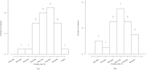
Histogram of the overlap ratios. (a) Histogram for the 32 lesions in the first dataset and (b) histogram for the 23 lesions in the second dataset.

About 12 out of 32 lesions were attached to the chest wall, and 11 out of 32 lesions were attached to the mediastinum. The average overlap ratios were 73% and 67%, respectively. Figures 5a, 5b, 5c, 5d showed four of those cases attaching to the chest wall and/or mediastinum in a center slice with computer results overlaid on the images. The overlap ratios were 79%, 59%, 61%, and 64%, respectively.

Figure 5.

Computer segmentation results. The upper row showing four lesions attaching to chest wall or mediastinum; the lower row showing four part-solid or GGO lesions. OR denoting overlap ratio. The inner contour on (e) showing a cavity excluded from the volume of the lesion.

About 6 out of 32 lesions were part-solid or GGO lesions. The average overlap ratio was 71% for solid lesions and 60% for part solid or GGO lesions. Figures 5e, 5f, 5g, 5h show four examples of the GGO cases with overlap ratios of 82%, 44%, 71%, and 33%, respectively. Figure 5h shows a dumbbell shaped tumor (possibly due to the merging of two tumors); the algorithm captured half of it, resulting in a low overlap ratio.

Although the algorithm was trained with large lesions, when applied to the substantially smaller lesions of the first LIDC dataset, it achieved an average overlap ratio of 65%. The distribution of the overlap ratio is shown in Fig. 4b. The minimum overlap value was 39%, as shown in Fig. 6a; the maximum overlap ratio was 90%, as shown in Fig. 6d. Figures 6b, 6c show an irregular shaped nodule and a juxtapleural nodule with overlap ratios 63% and 75%, respectively. Figure 6a shows a small ground glass nodule with an ill-defined boundary that posed a challenge to radiologists; the region with 50% or greater consensus was much smaller than the computer segmented region, resulting in a low overlap ratio.

Figure 6.

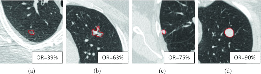
Computer segmentation result on four LIDC nodules. OR denoting overlap ratio. (a) A ground glass nodule having the minimum overlap ratio, (b) a part-solid irregular nodule, (c) a juxtapleural nodule, and (d) an isolated nodule having the maximum overlap ratio.

The relative difference versus the true phantom volumes is shown in Fig. 7. The relative difference was greater for smaller nodules than larger nodules. The average relative difference was −3%, and the 95% limit of agreements was −21%, 15%. Figure 8 showed the segmentation results of three phantom nodules (lobulated 10 mm –630 HU, speculated 20 mm 100 HU, and spherical 20 mm 100 HU), with relative difference 1%, −7%, and 0.4%, respectively.

Figure 7.

Relative difference versus true volume of the phantom nodules.

Figure 8.

Segmentation results on three phantom nodules. RD denoting relative difference. (a) A −630 HU lobulated nodule, (b) a 100 HU spiculated nodule, and (c) a 100 HU spherical nodule.

The coffee-break dataset was used to assess the algorithm's test-retest reliability. Statistically, test-retest reliability assesses consistency and reproducibility of repeated measurements. The ICC described the proportion of total variation due to variation between prewalk and postwalk scans. The ICC was 0.998 with 95% confidence interval between 0.995 and 0.999.

Average segmentation time was 13 s for the coffee-break dataset on a Hewlett-Packard Z800 workstation with CPU clocked at 2.67 GHz. The lesions found in the coffee-break dataset were large in diameter. The algorithm ran faster for smaller lesions.

DISCUSSION

Segmentation of small pulmonary nodules detected in lung cancer screening programs has been intensively studied.^{5, 6, 7, 8, 9, 10, 14, 16} Unlike those small pulmonary nodules, lesions found in patients with lung cancer are often large and vary considerably in their shape, density, texture, and relationship to surrounding anatomic structures. Lesions may have portions of GGO, honeycombing, cavities, or other inhomogeneous patterns, and may be attached to areas of pneumonia, atelectasis, or anatomic structures such as the chest wall, vessels, or mediastinum. All these varying conditions make segmentation more challenging. The segmentation algorithm was trained primarily with 52 lesions from 48 patients with advanced lung cancer³ and refined over time through further application to a broader set of tumors from other lung cancer related studies, and demonstrated good segmentation performance when applied to small lung nodules detected in CT lung cancer screening programs and lung nodule phantoms of different size, shape, and density.

Our approach uniquely combines several techniques, advancing the particular advantages of each. Marker controlled watershed method is effective at finding edges, and the watershed lines often correspond to the strong edges between markers. However, the watershed lines are often irregular, and sometimes include vessels and other nonlesion structures. To detach vessels, techniques such as morphological operations can be applied, but often at the expense of boundary details. The boundary details can be recaptured by geometric active contours.

If there is a lack of a good initial contour, geometric active contours employ inflation or deflation forces to drive the contours outward or inward; however, the strength of the force can be difficult to determine. If the inflation force is too small, the contour stops too soon, resulting in undersegmentation; if the force is too large, the contours pass through the lesion boundary, resulting in oversegmentation. Deflation forces are prone to similar pitfalls. With a good initial contour, such as a contour from watershed segmentation, the need for an inflation or deflation force can be eliminated.

The above methods are edge based and may not capture the nodule's ground glass opacity regions, which often share blurred edges with the surrounding lung parenchyma. Markov random field can improve the segmentation of GGO or part-solid lesions, as demonstrated in Fig. 9. Unlike an edge-based method, the MRF method assumes that the image is generated from a random Markov field and seeks the most plausible random field that could generate the image.

Figure 9.

Refinement for a part-solid nodule by MRF. (a) The segmentation result before refinement and (b) the segmentation result on the same slice after refinement.

Lesions attached to chest wall or mediastinum were treated the same as other lesions. Previous studies employed the strategy of extracting the chest wall prior to segmenting pleural nodules and masses.^{10, 16, 29} However, techniques such as rolling ball³⁰ often failed for large pleural lesions; the mediastinum was often harder to segment correctly a priori when a lesion was attached to it. We chose to not include an ad hoc chest wall extraction step prior to segmentation because any error in chest wall segmentation, often the more challenging task, could negatively affect lung lesion segmentation. Our algorithm relies on watershed transform, which can detect weak edges between markers and divide the plateau according to distance to markers in the instances when there is no edge at all.

Part-solid lesions were treated differently than solid lesions because their boundaries were often not well-defined. Whereas an edge-based method worked well with solid lesions, a probability-based method, specifically Markov random field, improved the GGO portion segmentation with part-solid lesions. The average overlap ratio of part-solid lesions was lower, which has two explanations. First, the GGO lesions were generally smaller in size than solid lesions in cancer patients, and smaller lesions tended to have smaller overlap ratios. Second, their indistinct boundaries made it more difficult for the computer and radiologist to agree on a boundary.

As each organ or type of tissue holds a fixed range of Hounsfield Units, some fixed parameters were used in this study. For example, we used a threshold of −150 HU to classify solid and nonsolid lesions, as it is lower than the density of fat and higher than the mean density of GGO. For GGO quantification, some studies applied a density mask with attenuation from −750 to −300 HU,³¹ while we found that a mean of −400 HU and a standard deviation of 200 HU suited our application. Choosing the distribution parameters adaptively for each tumor can sometimes improve the accuracy, but a wrong estimation of the parameters can result in including a large portion of inflammation of the lung.

The LIDC project provides annotated lesions for algorithm evaluation. Way et al. proposed a method based on 3D active contours.¹⁶ When their algorithm, which was trained on their own data, was applied to the first LIDC dataset, a mean overlap ratio of 58% was achieved. Tachibana and Kido developed a method based on threshold, watershed, and distance transformation.³² They trained and tested their algorithm with the first LIDC dataset, and achieved a mean overlap ratio of 51%. Wang et al. proposed a method based on spiral scanning and dynamic programming. They trained their algorithm with the first LIDC dataset, and achieved a mean overlap ratio of 66%.¹⁴ Our algorithm was trained with lesions from clinical trials that were much larger in diameter than the lesions in the LIDC dataset, and we achieved an overlap ratio of 65%.

Besides accuracy, the reliability of an algorithm is critical. A reliable algorithm should yield similar results under similar conditions. The high intraclass correlation coefficient our algorithm achieved on the coffee-break dataset indicates its reliability.

The active contours method we applied is a local optimization method that is sensitive to the initial contour. We relied on the marker-controlled watershed method for a good initial contour. When the watershed surface was far from the lesion boundary, the active contour was often attracted by local minimums rather than lesion boundary.

Our approach showed difficulty separating lesion tissue from obstructive pneumonia, atelectasis, or other kinds of nonmalignant consolidation. These abnormalities challenged the radiologists as well because little if any contrast exists between lesion and consolidation on CT images. If a lesion presented a honeycombing pattern, the algorithm could be misled by nonlesion edges, and the overlap ratio would also be low.

The RIDER dataset and the phantom dataset are reconstructed at 1.25 mm slice thickness with sharp convolution kernel. The convolution kernels for the 23 LIDC cases were unknown; 22 were reconstructed at 0.625 mm slice thickness and one was at 2.5 mm slice thickness. Further studies are warranted to study the effect of different image acquisition parameters on the segmentation result.

CONCLUSION

In this work we proposed a novel technique to segment lung lesions on CT images that incorporates watershed transform, geometric active contours, and Markov random field. The algorithm proved highly accurate and reliable when applied to a wide range of lesions, small or large, solid or part-solid, solitary or juxtapleural. This method would be valuable for lesion contour delineation and volumetric quantification in clinical applications such as treatment planning and therapy response assessment.

References

- Jemal A., Siegel R., Xu J., and Ward E., “Cancer statistics, 2010,” Ca-Cancer J. Clin. 60(5), 277–300 (2010). 10.3322/caac.20073 [DOI] [PubMed] [Google Scholar]
- Therasse P., Arbuk S. G., Eisenhauer E. A., Wanders J., Kaplan R. S., Rubinstein L., Verweij J., Van Glabbeke M., van Oosterom A. T., Christian M. C., and Gwyther S. G., “New guidelines to evaluate response to treatment in solid tumors,” J. Natl. Cancer Inst. 92, 205–216 (2000). 10.1093/jnci/92.3.205 [DOI] [PubMed] [Google Scholar]
- Zhao B., Oxnard G. R., Moskowitz C. S., Kris M. G., Pao W., Guo P., Rusch V. M., Ladanyi M., Rizvi N. A., and Schwartz L. H., “A pilot study of volume measurement as a method of tumor response evaluation to aid biomarker development,” Clin. Cancer Res. 16, 4647–4653 (2010). 10.1158/1078-0432.CCR-10-0125 [DOI] [PMC free article] [PubMed] [Google Scholar]
- Mozley P. D., Schwartz L. H., Bendtsen C., Zhao B., Petrick N., and Buckler A. J., “Change in lung tumor volume as a biomarker of treatment response: A critical review of the evidence,” Ann. Oncol. 21, 1751–1755 (2010). 10.1093/annonc/mdq051 [DOI] [PubMed] [Google Scholar]
- Zhao B., Reeves A., Yankelevitz D., and Henshke C., “Three-dimensional multi-criterion automatic segmentation of pulmonary nodules of helical computed tomography images,” Opt. Eng. 38, 1340–1347 (1999). 10.1117/1.602176 [DOI] [PubMed] [Google Scholar]
- Zhao B., Yankelevitz D., Reeves A., and Henschke C., “Two-dimensional multi-criterion segmentation of pulmonary nodules on helical CT images,” Med. Phys. 26, 889–895 (1999). 10.1118/1.598605 [DOI] [PubMed] [Google Scholar]
- Zhao B., Kostis W. J., Reeves A. P., Yankelevitz D. F., and Henschke C. I., “Consistent segmentation of repeat CT scans for growth assessment in pulmonary nodules,” Proc. SPIE. 3661, 1012–1018 (1999). 10.1117/12.348494 [DOI] [Google Scholar]
- Kostis W. J., Reeves A. P., Yankelevitz D. F., and Henschke C. I., “Three-dimensional segmentation and growth-rate estimation of small pulmonary nodules in helical CT images,” IEEE Trans. Med. Imaging 22, 1259–1274 (2003). 10.1109/TMI.2003.817785 [DOI] [PubMed] [Google Scholar]
- Mullally W., Betke M., Wang J., and Ko J. P., “Segmentation of nodules on chest computed tomography for growth assessment,” Med. Phys. 31, 839–848 (2004). 10.1118/1.1656593 [DOI] [PubMed] [Google Scholar]
- Reeves A., Chan A., Yankelevitz D., Henschke C., Kressler B., and Kostis W., “On measuring the change in size of pulmonary nodules,” IEEE Trans. Med. Imaging 25, 435–450 (2006). 10.1109/TMI.2006.871548 [DOI] [PubMed] [Google Scholar]
- S.ArmatoIII, McLennan G., McNitt-Gray M., Meyer C., Yankelevitz D., Aberle D., Henschke C., Hoffman E., Kazerooni E., MacMahon H., Reeves A., Croft B., and Clarke L., “Lung image database consortium: Developing a resource for the medical imaging research community,” Radiology 232, 739–748 (2004). 10.1148/radiol.2323032035 [DOI] [PubMed] [Google Scholar]
- Zhao B., Schwartz L. H., Moskowitz C., Ginsberg M. S., Rizvi N. A., and Kris M. G., “Computerized quantification of tumor response in lung cancer: Initial results,” Radiology 241, 892–898 (2006). 10.1148/radiol.2413051887 [DOI] [PubMed] [Google Scholar]
- Dehmeshki J., Amin H., Casique M. V., and Ye X., “Segmentation of pulmonary nodules in thoracic CT scans: A region growing approach,” IEEE Trans. Med. Imaging 27, 467–480 (2008). 10.1109/TMI.2007.907555 [DOI] [PubMed] [Google Scholar]
- Wang J., Engelmann R., and Li Q., “Segmentation of pulmonary nodules in three-dimensional CT images by use of a spiral-scanning technique,” Med. Phys. 34, 4678–4689 (2007). 10.1118/1.2799885 [DOI] [PubMed] [Google Scholar]
- Kass M., Witkin A., and Terzopoulos D., “Snakes: Active contour models,” Int. J. Comput. Vis. 1, 321–331 (1988). 10.1007/BF00133570 [DOI] [Google Scholar]
- Way T., Hadjiiski L., Sahiner B., Chan H., Cascade P., Kazerooni E., Bogot N., and Zhou C., “Computer-aided diagnosis of pulmonary nodules on CT scans: Segmentation and classification using 3D active contours,” Med. Phys. 33, 2323–2337 (2006). 10.1118/1.2207129 [DOI] [PMC free article] [PubMed] [Google Scholar]
- Vincent L. and Soille P., “Watersheds in digital spaces – An efficient algorithm based on immersion simulations,” IEEE Trans. Pattern Anal. Mach. Intell. 13, 583–598 (1991). 10.1109/34.87344 [DOI] [Google Scholar]
- Vincent L., “Morphological grayscale reconstruction in image analysis: Applications and efficient algorithms,” IEEE Trans. Image Process. 2, 176–201 (1993). 10.1109/83.217222 [DOI] [PubMed] [Google Scholar]
- Felzenszwalb P. F. and Huttenlocher D. P., “Distance transforms of sampled functions,” Cornell Computing and Information Science Technical Report TR2004-1963, 2004.
- Yezzi A., Kichenessamy S., Kumar A., Olver P., and Tannenbaum A., “A geometric snake model for segmentation of medical imagery,” IEEE Trans. Med. Imaging 16, 199–209 (1997). 10.1109/42.563665 [DOI] [PubMed] [Google Scholar]
- Caselles V., Kimmel R., and Sapiro G., “Geodesic active contours,” Int. J. Comput. Vis. 22, 61–79 (1997). 10.1023/A:1007979827043 [DOI] [Google Scholar]
- Zhao H. K., Chan T. F., Merriman B., and Osher S., “A variational level set approach to multiphase motion,” J. Comput. Phys. 127, 179–195 (1996). 10.1006/jcph.1996.0167 [DOI] [Google Scholar]
- Huisken G. and Sinestrari C., “The volume preserving mean curvature flow,” J. Reine Angew. Math. 382, 35–48 (1987). 10.1515/crll.1987.382.35 [DOI] [Google Scholar]
- Geman S. and Geman D., “Stochastic relaxation, Gibbs distributions and the Bayesian restoration of images,” IEEE Trans. Pattern Anal. Mach. Intell. 6, 721–741 (1984). 10.1109/TPAMI.1984.4767596 [DOI] [PubMed] [Google Scholar]
- Zhu Y., Tan Y., Hua Y., Zhang G., and Zhang J., “Automatic segmentation of ground-glass opacities in lung CT images by using Markov random field-based algorithms,” J. Digit. Imaging 25, 409–422 (2011). 10.1007/s10278-011-9435-5 [DOI] [PMC free article] [PubMed] [Google Scholar]
- Zhao B., James L. P., Moskowitz C., Guo P., Ginsberg M. S., Lefkowitz R. A., Qin Y., Riely G. J., Kris M. G., and Schwartz L. H., “Evaluating variability in tumor measurements from same-day repeat CT scans in patients with non-small cell lung cancer,” Radiology 252, 263–272 (2009). 10.1148/radiol.2522081593 [DOI] [PMC free article] [PubMed] [Google Scholar]
- Gavrielides M. A., Kinnard L. M., Myers K. J., Peregoy J., Pritchard W., Zeng R., Esparza J., Karanian J., and Petrick N., “A resource for the assessment of lung nodule size estimation methods: Database of thoracic CT scans of an anthropomorphic phantom,” Opt. Express 18(14), 15244–15255 (2010). 10.1364/OE.18.015244 [DOI] [PMC free article] [PubMed] [Google Scholar]
- McGraw K. and Wong S., “Forming inferences about some intraclass correlation coefficients,” Psychol. Methods 1, 30–46 (1996). 10.1037/1082-989X.1.1.30 [DOI] [Google Scholar]
- Zhao B., Schwartz L. H., Lefkowitz R. A., and Wang L., “Measuring tumor burden – Comparison of automatic and manual techniques,” Proc. SPIE 5370, 1695–1700 (2004). 10.1117/12.534342 [DOI] [Google Scholar]
- S. G.ArmatoIII, Giger M. L., and MacMahon H., “Automated lung segmentation in digitized posteroanterior chest radiographs,” Acad. Radiol. 5(4), 245–255 (1998). 10.1016/S1076-6332(98)80223-7 [DOI] [PubMed] [Google Scholar]
- Kauczor H.-U., Heitmann K., Heussel C. P., Marwede D., Uthmann T., and Thelen M., “Automatic detection and quantification of ground-glass opacities on high-resolution CT using multiple neural networks comparison with a density mask,” Am. J. Roentgenol. 175(5), 1329–1334 (2000). 10.2214/ajr.175.5.1751329 [DOI] [PubMed] [Google Scholar]
- Tachibana R. and Kido S., “Automatic segmentation of pulmonary nodules on CT images by use of NCI lung image database consortium,” Proc. SPIE 6144, 61440M (2006). 10.1117/12.653366 [DOI] [Google Scholar]