

Abstract
Diffuse optical imaging using non-ionizing radiation is a non-invasive method that shows promise towards breast cancer diagnosis. Hand-held optical imagers show potential for clinical translation of the technology, yet they have not been used towards 3D tomography. Herein, 3D tomography of human breast tissue in vivo is demonstrated for the first time using a hand-held optical imager with automated coregistration facilities. Simulation studies are performed on breast geometries to demonstrate the feasibility of 3D tomographic imaging using a hand-held imager under perfect (1:0) and imperfect (100:1, 50:1) fluorescence absorption contrast ratios. Experimental studies are performed in vivo using a 1 μM ICG filled phantom target placed non-invasively underneath the flap of the breast tissue. Results show the ability to perform automated tracking and coregistered imaging of human breast tissue (with tracking accuracy on the order of ~1 cm). Three-dimensional tomography results demonstrated the ability to recover a single target placed at a depth of 2.5 cm, from both the simulated (at 1:0, 100:1 and 50:1 contrasts) and experimental cases on actual breast tissues. Ongoing efforts to improve target depth recovery are carried out via implementation of transmittance imaging in the hand-held imager.
1. Introduction
Diffuse optical imaging using near-infrared (NIR) light is a promising technology which has been developed over the past three decades towards applications such as functional brain mapping and breast cancer diagnosis. The method is non-invasive, uses non-ionizing radiation, requires relatively inexpensive instrumentation, and provides functional information from in vivo biological tissues. Spectroscopic measurements of tissue optical properties can be obtained using a single source-detector pair which is termed as diffuse optical spectroscopy (DOS). Many sources and detectors over a large area are used to generate three-dimensional (3D) images toward diffuse optical imaging (DOI) and tomography (DOT). Additionally, an exogenous fluorescence contrast agent can be introduced into the tissue to produce a unique fluorescence (emission) signal towards detection of smaller and deeper lesions, as in fluorescence-enhanced optical imaging or fluorescence diffuse optical tomography (FDOT). Indocyanine green (ICG) is a fluorescing dye typically used for fluorescence-enhanced optical imaging studies in vivo (Godavarty 2003, Corlu 2007, Rasmussen 2009, selected references), because it is non-toxic at low concentrations and is approved by the Food and Drug Administration (FDA) for use in humans to asses hepatic function (Leevy 1967) and in retinal angiography( Kogure 1970).
Several research groups have developed optical systems for breast cancer imaging which have been tested on human subjects (Nioka 1997, Alacam 2008, Culver 2003, Corlu 2007, Choe 2005, Choe 2009, Van de Ven 2009a, Vav de Ven 2009b, Poellinger 2008, Grosenick 2003, Grosenick 2005, Taroni 2005a, Taroni 2005b, Taroni 2010, selected references). Many of the systems are composed of a bed on which the patient lies prone with the breast pendant in a circular hole or rounded cup which contains the sources and detectors in a circular or hemispherical geometry. Bed-based optical imaging systems have the advantage of performing 3D tomography due to the fixed geometry of source/detector locations. However, they also have limitations in that the systems are large and bulky, and the fixed geometry might not accommodate all breast sizes, and requires the use of matching fluid. In order to make the optical imaging technology more portable and patient-comfortable, several other groups have developed hand-held optical devices toward rapid clinical translation of the technology (Tromberg 1997, Cerussi 2006, Cerussi 2007, Chance 2005, Erickson 2009, Erickson 2011, selected references). To date, the focus of hand-held devices has been towards 2D spectroscopic imaging. The hand-held systems have the advantages of being portable and able to image any tissue size; however, they have not been used to perform 3D tomographic imaging. Tomography is desirable in order to perform 3D localization of the tumor which is useful in diagnosis, staging, and image-guided biopsy.
Performing 3D tomography using a hand-held device presents a challenge in that there is no fixed geometry and source-detector layout as in bed-based optical imaging systems. Three-dimensional tomography requires that precise locations of the optical measurements (i.e. source-detector locations) on the tissue surface be known. However, each human subject has different size and shape of the breast tissue and the source-detector locations change with each probe location during imaging. In our Optical Imaging Laboratory, a hand-held optical imaging system has been developed that has the following unique features: (i) it is able to contour to curved tissue surfaces, (ii) it uses simultaneous illumination and detection over a large (4 × 9 cm2) surface area towards rapid data acquisition, (iii) it has coregistration facilities to produce 3D surface optical images of the breast tissue in near-real time, (iv) it is able to perform 3D tomography. Tomography was possible from the unique coregistration facilities that enable real-time tracking of the hand-held probe’s location with reference to the tissue during imaging, and automate coregistration of the source-detector locations on to the discretized 3D tissue geometry. The system has previously demonstrated coregistered imaging (Regalado 2010) and 3D tomography in tissue phantoms (Ge 2008), as well as 2D imaging of fluorescent targets in human breast tissue (Erickson 2010). Herein, the ability of this hand-held optical imaging system to perform coregistered imaging as well as 3D tomographic imaging in vivo on human breast tissues is demonstrated. Fluorescence tomography studies from simulated and experimental cases in vivo on healthy breast tissues were carried out using the hand-held optical imaging system, and employing the approximate extended Kalman filter (AEKF) inversion algorithm (Fedele 2003, Godavarty 2003).
2. Materials and methods
Details of the instrumentation, data analysis, automated coregistration approach, 3D tomography approach, and the simulated and experimental studies performed are described in this section.
2.1 Instrumentation and data analysis
The three major components of the imaging system are the hand-held probe, the laser diode source, and an intensified charge-coupled device (ICCD) detector (shown in Figure 1). The instrumentation is developed such that it can acquire both continuous wave (CW) and frequency-domain photon migration (FDPM) optical measurements as required (Ge 2008). In the current tomography studies, CW measurements were acquired. The hand-held probe head is designed with unique features in that it is flexible to contour to different tissue curvatures, it has a 4 × 9 cm2 imaging area for large volume interrogation, and it uses simultaneous illumination and detection for rapid data acquisition of large tissue volumes. The hand-held probe face is shown in Figure 1 (inset). The probe is composed of three sections (or plates) and each of the side sections is capable of curving up to 45° (Ge 2008, Jayachandran 2007).
Figure 1.

Hand-held optical imaging system composed of the laser diode source, ICCD camera detector, and the hand-held probe head. Inset: The actual hand-held probe face showing the source-detector configuration. The large solid red dots represent the six source fiber locations and all other small dots are the 165 detector fiber locations. All the fiber locations are spaced 0.5 cm away from each other.
At the source end, a single 785-nm laser diode source (530 mW, HPD1005-9MM, Intense Ltd., North Brunswick, NJ) is split into six illuminating fibers using a custom-built collimator-diffuser package. The six illuminating fibers are coupled to the hand-held probe (at the six red dots’ location as shown in Figure 1 (inset)). At the detector end, a gain modulated image intensifier (FS9910, ITT Night Vision, VA) is optically coupled to the CCD camera (PI-SCX 7495-0002, Roper Scientific, Trenton, NJ). For fluorescence studies two band pass interference filters of blocking OD 4 and 6 (HRF-830.0, blocking OD 6 and F-830.0, blocking OD 4, CVI Laser, Albuquerque, NM) are used. Two synthesizers are connected at the source and detector end to modulate the signal for FDPM measurements as required. The instrumentation is described in more detail elsewhere (Ge 2008).
During imaging, the hand-held probe is placed in full contact with the tissue being imaged (with the probe in the flat position for the cases described here). Herein, fluorescence intensity images are acquired using ICG as the extrinsic fluorescence contrast agent. The raw fluorescence intensity images at the ICCD camera end were acquired in 1-sec (0.2 sec exposure time of the ICCD camera × 5 repeated measurements, or frames). These images were post-processed (~1 sec) to produce the fluorescence intensity distribution of the detector fibers at the probe face as 2D contour plots (i.e. 2D surface images) using in-house developed Matlab codes. A subtraction-based post-processing technique was employed on each image in order to eliminate excitation leakage, only for experimental cases (Ge 2008). Background subtraction was performed by subtracting the optical intensity data of an image of the breast tissue without a fluorescent target from an image with a fluorescent target (placed non-invasively under the flap of the breast tissue).
2.2 Automated coregistered imaging and 3D tomography
Three-dimensional tomographic imaging is feasible when the 3D coordinates of the acquired surface optical measurements are known with respect to the imaged tissue geometry. This was achieved by implementing coregistered imaging via real-time tracking of the hand-held probe’s location, such that the 3D coordinates of the source/detector locations are obtained in parallel to the optical measurements.
2.2.1 Automated coregistered imaging
Coregistered imaging involves registering the acquired subtracted fluorescence intensity image onto its true imaged location, using the 3D positional information (as obtained from a motion tracker). Coregistration was carried out as a four-step process, as illustrated in Figure 2. In step 1, the breast tissue geometry was acquired using a 3D scanner and discretized into a 3D surface mesh. A commercially available hand-held 3D scanner (Fastscan, Polhemus, Inc.) was employed, and approved for human subjects’ scanning by the University’s (FIU) Institutional Review Board. The scanner was installed on a custom-developed motorized railing (in a curtained room) to allow hands-free operator independent scanning and privacy for the subjects. Each scan was composed of a series of four sweeps of the scanner which would cover both sides of the breast tissue as well as part of the chest wall and ribcage area. The scan was displayed on the computer screen as a 3D surface geometry and MATLAB software developed in-house was used to generate a discretized surface mesh. This discretized mesh (shown in Figure 2, Step 1) was in turn imported into the custom-developed coregistration software for imaging (Regalado 2010) In order to perform 3D tomography, a 3D volume was generated from the scanned surface geometry using GiD software (Barcelona, Spain) and a tetrahedral mesh was generated using FLUENT’s Gambit software. In step 2, the position and orientation of the hand-held probe was tracked using an acoustic-based motion tracker in real-time using MATLAB/LabVIEW software. The software was developed in house to determine the probe’s location with respect to the tissue geometry (shown in Figure 2, Step 2). In step 3, a real-time 2D surface contour image of detected optical signals (here CW fluorescence intensity) was acquired at a given probe location using the hand-held imager (as described in Section 2.1 and shown in Figure 2, Step 3). In each case, two images were collected, one with the fluorescent target and a background image without the target. The background image was subtracted to remove noise, prior to the coregistration step. In step 4, the 2D surface contour plot from Step 3 is coregistered (shown in Figure 2, Step 4) onto the discretized breast tissue geometry at the respective probe location using the 3D positional information of the probe (i.e. all source and detector point locations), as obtained from Step 2. The entire coregistration procedure is explained in more detail elsewhere (Regalado, 2010).
Figure 2.
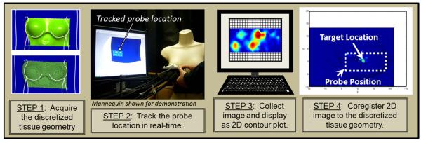
The 4-step in vivo coregistered imaging process carried out during in vivo optical imaging studies on breast tissues.
2.2.2 Accuracy of 3D positional tracking
The accuracy of the tracked location of the probe was quantitatively determined for curved breast tissue geometries. To validate the coregistration process, reference points were placed in the discretized breast geometry and the corresponding locations were measured with a ruler and marked on the tissue of the subject (Figure 3). The center (nipple) region of the left breast was arbitrarily selected to be the origin and used as such for all studies. The probe was placed at the initial position where the probe origin (bottom left corner of the probe face) was aligned with the tissue origin. The probe origin was then moved to the different reference points of known [x,y,z] coordinates (shown in Figure 3) and the tracking position was recorded (10 repetitions at each location). The distance formula in three dimensions was used to determine the discrepancy between the tracked and true locations. Once the probe was placed at a desired location, an image was collected and the tracked positional information was used to coregister the image by calculating the closest node in the breast surface mesh geometry to each 3D positional location of the sources/detectors on the probe. Hence the accuracy of coregistered imaging was dependent on the accuracy of the tracker as well as the coarseness of the node separation in the breast mesh geometry.
Figure 3.

Schematic of the breast tissue and probe placement during accuracy studies of probe localization. The location of the reference points within a coordinate system (in cm) are shown, where the center (nipple) region of the left breast was arbitrarily selected to be the origin and used as such for all studies. The green dotted rectangle shows the initial probe position where the probe origin (bottom left corner of the probe face) is aligned with the initial reference point (chosen as the origin of the coordinate system). The probe origin was then placed over each of the other reference points marked on the tissue and the tracked location was recorded. Figure not to scale.
2.2.3 Three-dimensional tomography in human breast tissue
Three-dimensional fluorescence tomographic imaging employs the coregistered optical (here, CW fluorescence intensity) measurements, the coupled diffusion equations (that represent the light propagation in tissues) and an inversion algorithm (here, approximate extended Kalman filter, AEKF) in order to reconstruct the 3D optical property maps of the tissue geometry. A flow diagram of the 3D tomography approach performed for the current breast imaging studies is shown in Figure 4.
Figure 4.

Flow diagram of steps involved in 3D tomographic imaging in vivo. The input from the red dashed box to the AEKF algorithm are the coregistered optical measurements.
The coregistered image of optical intensity data (detailed in section 2.2.1 above) was acquired from the breast tissue using the hand-held optical imager. A 3D volume of the breast tissues (both left and right) was rendered from the scanned 3D breast surface geometry (as described in section 2.2.1). The volume was truncated such that only the section of interest (i.e. left or right breast) was used in the image reconstructions, thus reducing computational time. A 3D tetrahedral unstructured volume mesh was generated from the 3D volume geometry. The mesh contained 8877 nodes, 7569 surface elements, and 41371 volume elements. The element size was 5 mm at the surface and 10 mm in the volume. The smaller element size was used at the surface to correspond to the 5 mm spacing of the detectors in the probe face, and the larger element size was used in the volume in order to reduce the computational time. In future, smaller element sizes can be used to improve the accuracy of the reconstruction. The source and detector node numbers were extracted from the 3D breast mesh, using their positional information as obtained from the coregistered images. The fluorescence intensity data (of the five repeated measurements corresponding to one image) was correlated to its respective detector location in the 3D coordinate system of the tissue geometry. Average optical property values of human breast tissue acquired from the literature (μa=0.05 cm−1, μs’=8.0 cm−1) (Leff 2008) were used in the image reconstructions. Finally, all the information from these steps (indicated in the flow diagram by the red dashed line) is input into a computationally efficient version of an approximate extended Kalman filter (AEKF) inversion algorithm (Godavarty 2003). The algorithm was used to reconstruct the 3D optical property map of the absorption coefficient due to the fluorophore at excitation wavelength (μaxf). The complete AEKF algorithm has been described in detail elsewhere (Godavarty 2003, Fedele 2003), and is briefly described here in regards to the application to in vivo data.
The fluorescence optical measurements (as obtained from the coregistered image, shown in the red dashed box of Figure 4) and the 3D volume mesh are input only once at the start of the program (i=1). The coupled diffusion equations representing the light propagation at the excitation and emission wavelengths is used during image reconstructions. For the forward simulations (employing the coupled diffusion equations), in the first iteration (i=1), the parameter of interest (here μaxf) is considered uniform and constant in the entire 3D volume mesh (arbitrarily chosen here as 0.003 cm−1). Along with the experimental measurements and coupled diffusion equations, the inversion algorithm also accounts for measurement error, model error and parameter error. Measurement error is estimated as the covariance across the five repeated measurements, and input as the measurement error covariance in the inversions. The model error covariance (which occurs due to simplifications in the forward model) was empirically chosen to be one-fourth the mean of the measurement covariance (Godavarty 2003). Parameter error is the error in the unknown spatially distributed parameter values μaxf, and was initially set to 0.1 for the studies performed here. The AEKF algorithm recursively minimizes the variance of the parameter error, which in this case the parameter is μaxf, to get an updated parameter distribution and forward simulation at each iteration (i=i+1). The convergence criterion is met when the RMSE (root mean square output error) is less than 1%, or the total number of iterations exceeds 50. The reconstructed parameter μaxf of the entire breast tissue volume was presented as iso-surface contour plots to qualitatively show the reconstructed target location. The recovered and true centroid locations (or approximate true centroid location for the case of in vivo experimental data) were compared using the distance formula. The recovered centroid location was determined by the weighted sum of the x,y,z values containing a μaxf value above the cutoff. A cutoff value based on the first break point in the histogram plot of μaxf was used to differentiate the target from background. The reconstructed target volume with respect to background was quantitatively estimated as the total volume of all the volume elements whose μaxf value was above the cutoff (Godavarty 2003).
2.3 Experimental studies
Fluorescence-enhanced optical imaging studies were performed on a healthy female (with no breast cancer). The experimental studies were carried out using a phantom (ICG) target placed non-invasively underneath the flap of the breast tissue (to mimic a breast cancer case) in order to test the ability of the device in detecting/imaging a target through actual human breast tissue (Erickson 2010). Herein, a healthy female subject above age 21 was recruited for the study (approved by the FIU Institutional Review Board). The subject was seated in an upright 90° position and the probe was placed on the breast tissue with enough compression to ensure full contact. The imaging set-up is shown in Figure 2 (Step 2). A 0.45 cm3 volume (0.95 cm diameter) spherical target filled with 1 μM ICG (in 1% Liposyn solution) was superficially placed underneath the flap of the breast tissue (Figure 5) at different clock positions in different experimental cases. The probe was placed in full contact with the breast tissue and CW images of fluorescence intensity were acquired and automatically coregistered with respect to their imaged location on the tissue geometry. The 2D subtracted fluorescence image was acquired in ~5 sec imaging and post-processing time (as described in section 2.1) and the coregistration time required ~30 seconds for a total time of ~35 seconds to acquire one coregistered image. The coregistered image (obtained from a single location) was then used to reconstruct the 3D optical property map of the fluorescent target within human breast tissue geometry. The recovered location, volume, and target to background (T:B) ratio were compared w.r.t their true values. For these experimental cases, the true target location was an approximation as the target was placed under the tissue in the dark and minor shifting of the target may occur as the probe was placed on the tissue. Hence simulation studies were performed as well to test the ability (and accuracy) to perform 3D tomography studies using a hand-held imager (as described in the next section).
Figure 5.

Schematic showing the location of a fluorescent target placed superficially underneath the breast tissue and the location of the probe during imaging.
2.4 Simulated Studies
Simulation studies were performed using the coupled diffusion equation for continuous-wave, fluorescence intensity measurements. Simulated data sets were generated using a Galerkin-based FEM (finite element method) forward model (as in the AEKF reconstruction algorithm), without Gaussian noise addition in order to mimic an ideal case. Simulation studies were carried out on 3D breast geometries by assuming targets of varying volumes placed inside the breast geometry at different clock positions in each case. The depth of the target was measured with respect to the breast surface and represented by the x-axis. The y- and z- axis are the horizontal and vertical axis, respectively. A 1% noise was added across the five repeated simulated measurements to mimic measurement errors of an experimental case. Experimental studies were performed under perfect (1:0) and imperfect (100:1 and 50:1) fluorescence uptake contrast ratios in order to mimic both tumor-specific as well as non-specific fluorescence contrast agents, respectively. The source and detector locations of the probe were extracted from the coregistered data acquired during imaging of a human subject and a simulated data set was substituted for the experimental data in order to quantitatively evaluate the ability to recover a target close to the known location. A perfect uptake case is not a true representation of a clinical case since ICG is a blood pooling agent and some fluorescent signal would be present in the background. The experimental studies performed in vivo herein show perfect uptake since the fluorescing agent was only injected in the phantom target and not into the actual human subject. In order to demonstrate a more realistic imperfect uptake case, 3D reconstructions were performed with simulated data of tumor-to-background ratios (T:B) of 100:1 and 50:1. The details for all simulation and experimental tomography cases are provided in Table 1.
Table 1.
Summary of 3D fluorescence-enhanced optical tomography studies (simulated and experimental).
| Case # | Data Type | Target Volume (cm3) | T:B | Target Location (x, y, z)[cm] or clock position |
|---|---|---|---|---|
| 1 | Simulated Data | 0.45 | 1:0 | (2.5, 0, 0) |
| 2 | Simulated Data | 0.45 | 1:0 | (2.5, -4, -1) |
| 3 | Simulated Data | 0.23 | 1:0 | (2.5, 2.5, -1) |
| 4 | Simulated Data | 0.45 | 100:1 | (2.5, 0, 0) |
| 5 | Simulated Data | 0.45 | 50:1 | (2.5, 0, 0) |
| 6 | Experimental Data | 0.45 | 1:0 | ~ 6 o’clock |
| 7 | Experimental Data | 0.45 | 1:0 | ~ 4 o’clock |
| 8 | Experimental Data | 0.23 | 1:0 | ~ 8 o’clock |
3. Results
3.1 Accuracy of 3D positional tracking
The average and standard deviation of the tracked location in 3D, and its total distance-off from the true location at each position is given in Table 2. It can be seen from the standard deviation of the measured values that the tracked probe position fluctuates between 0.06-0.4 cm (across 10 repeated measurements at each coordinate). The standard deviation at positions 2 and 3 (see Figure 4) were greater than at positions 1 and 4, which is likely due to the various contours of the human body at the different probe locations. Location 1 and 4 correspond to the left breast tissue and ribcage, respectively, and location 2 and 3 correspond to the right breast tissue and the chest wall between the breasts, respectively. Since the bottom left corner of the probe was aligned with the marked location, the probe was in a more steady position at locations 1 and 4 than at locations 2 and 3. The probe was steadier at location 1 than location 3 because it was supported by the chest wall. The average total distance off between the true and tracked location is ~1 cm, which is much higher than that previously determined from a cubical phantom (~0.19 cm) (Erickson 2010b). This can be attributed to: (i) instability in the tracker leading to fluctuations in the tracked position of the probe (Regalado 2010, Martinez 2010); and (ii) human error such as hand movement of the operator across the 10 measurement repetitions and manual measurement of the reference points on the tissue. Currently, efforts are made to overcome these limitations and improve the accuracy of the tracking coordinates.
Table 2.
Average and standard deviation of x,y,z coordinates (where x is the depth) as displayed by the tracking software and total distance off between true and measured values. Ten measurements were recorded at each position due to the fluctuation in readings from the instrument. The overall procedure was performed once.
| Location | True Value (x,y,z) cm |
Average Measured Value & Standard Deviation (x,y,z) cm |
Total Distance Off (cm) |
|---|---|---|---|
| 1 | (0, 0, 0) | (-0.18±0.09, -0.38±0.08, 0.31±0.10) | 0.53 |
| 2 | (0, -10, 0.5) | (-0.87±0.18, -9.19±0.33, 1.12±0.27) | 1.34 |
| 3 | (0, -20, 0) | (-0.44±0.20, -19.58±0.31, -0.15±0.41) | 0.63 |
| 4 | (1, -9, -8) | (0.29±0.06, -9.95±0.15, -8.87±0.07) | 1.47 |
3.2 Coregistered imaging in human subjects
The positional information from the tracked probe location and fluorescence intensity data from the hand-held imager were in turn used to generate the coregistered images. Figure 6 shows results for coregistered imaging studies performed on a healthy subject. A spherical target filled with 1 μM ICG (in 1% Liposyn solution) was placed underneath the flap of the breast tissue and fluorescence intensity images were collected and automatically coregistered using the positional tracking system. Figure 6A shows the coregistered fluorescence intensity image onto the discretized (3D surface) breast geometry (shown in blue) for Case #1. The probe position is indicated by the yellow dotted line and is overlaid for better visualization of the imaged location. The regions of higher fluorescence (shown as red in the figure) are close to the estimated target location. The elongation of the signal or (additional point of intensity) can be attributed as artifacts incurred as a result of the non-uniform intensity distribution among the six simultaneously illuminating sources as well as the movement of the tissue between the images obtained with and without the target. Figure 6B shows a zoomed image of 6A (Case #1). Figure 6C-D shows the resulting coregistered images for Case #2-3, respectively. The results show that a 0.23-0.45 cm3 target was detected through ~2.5 cm (depth) of human breast tissue and coregistered at the probe’s location on the tissue geometry.
Figure 6.

Coregistered images of fluorescence intensity data (in arbitrary units) collected from a healthy subject with an ICG-filled target using the initial set-up (subject seated in upright position). (A) Location of probe and coregistered image relative to the subject for Case #1. (B) Zoomed image for Case#1: 0.45 cm3 target at the 6 o’clock position. (C) Case #2 image: 0.45 cm3 target at the 4 o’clock position. (D) Case #3 image: 0.23 cm3 target at the 8 o’clock position. All targets contain 1 μM ICG (in 1% Liposyn solution). The yellow dotted line was overlaid to estimate the probe location (not to scale). The images show the fluorescence intensity coregistered to the location of the probe (source and detector positions) with respect to the (discretized) scanned tissue geometry. Subtraction was used prior to coregistration to remove background noise in all cases.
3.3 Three dimensional tomography in human breast tissue
Results are presented herein for simulated and experimental cases. Figure 7 shows the iso-surface contour plots of the reconstructed μaxf for simulated cases (within real breast tissue geometry) under perfect uptake (Cases #1-3 in Table 1). [s0]The quantitative reconstruction results of the recovered target’s location and volume, its distance off from true location, and recovered T:B ratio are given in Table 3.
Figure 7.

Iso-surface plots of the reconstructed μaxf values for the in vivo reconstruction using simulated data for (A) Case #1, where a 0.45 cm3 (0.95 cm diameter) fluorescent target placed at (x,y,z)=(2.5,0,0) cm to roughly estimate the 6 o’clock position (to mimic the in vivo experimental case #6) about 2.5 cm deep in the breast tissue, (B) Case #2, where a 0.45 cm3 (0.95 cm diameter) fluorescent target placed at (x,y,z)=(2.5,-4,-1) cm to roughly estimate the 4 o’clock position (to mimic the in vivo experimental case #7) about 2.5 cm deep in the breast tissue, and (C) Case #3, where a 0.23 cm3 (0.76 cm diameter) fluorescent target placed at (x,y,z)=(2.5,2.5,-1) cm to roughly estimate the 8 o’clock position (to mimic the in vivo experimental case #8) about 2.5 cm deep in the breast tissue. The black circle represents the true target location that was placed with respect to the clock positions (shown by the dashed cross-wire).
Table 3.
Quantitative results for the in vivo reconstructions using simulated and experimental data. Cases #6-8 represent experimental data where the target location is estimated by clock position and tentative (x,y,z) values are given to roughly mimic the coordinates of the clock positions relative to the breast geometry.
| # | Data Type | Actual Target Location (x,y,z) cm |
Actual Target Volum e (cm3) |
Actual T:B |
Recovered Target Location (x,y,z) cm |
Recovered Target Volume (cm3) |
Recovere d T:B |
Total Dista nce Off (cm) |
|---|---|---|---|---|---|---|---|---|
| 1 | Simulated | (2.5, 0, 0) | 0.45 | 1:0 | (1.05, 0, -0.66) | 1.11 | 240:1 | 1.59 |
| 2 | Simulated | (2.5, -4, -1) | 0.45 | 1:0 | (2.33, -4.48, -1.16) | 0.68 | 120:1 | 0.53 |
| 3 | Simulated | (2.5, 2.5, -1) | 0.23 | 1:0 | (2.21, 2.19, -1.02) | 0.72 | 190:1 | 0.43 |
| 4 | Simulated | (2.5, 0, 0) | 0.45 | 100:1 | (1.18, -0.02, -0.68) | 1.00 | 6:1 | 1.49 |
| 5 | Simulated | (2.5, 0, 0) | 0.45 | 50:1 | (1.18, 0.08, -0.84) | 0.63 | 1:1 | 1.57 |
| 6 | Experimental | ~ 6o’clock | 0.45 | 1:0 | (1.25, -1.14, -1.21) | 0.92 | 78:1 | N/A |
| 7 | Experimental | ~ 4 o’clock | 0.45 | 1:0 | (2.97, -5.40, -0.68) | 0.36 | 7:1 | N/A |
| 8 | Experimental | ~ 8 o’clock | 0.23 | 1:0 | (0.87, -1.56, -1.82) | 0.12 | 16:1 | N/A |
Figure 8 shows the iso-surface contour plots of the reconstructed μaxf for simulated cases (within real breast tissue geometry) under imperfect uptake (Cases #4-5 in Table 1). The quantitative reconstruction results are tabulated in Table 3.
Figure 8.
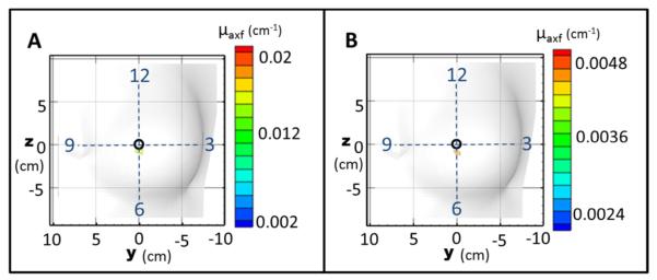
Iso-surface plots of the reconstructed μaxf values for the in vivo reconstruction using simulated data for (A) Case #4, where a 0.45 cm3 target was placed at (x,y,z)=(2.5,0,0) cm (corresponding to the 6 o’clock position) with T:B=100:1 and (B) Case #5, where a 0.45 cm3 target was placed at (x,y,z)=(2.5,0,0) cm (corresponding to the 6 o’clock position) with T:B=50:1. The black circle represents the true target location that was placed with respect to the clock positions (shown by the dashed cross-wire).
Figure 9 shows the iso-surface contour plots of the reconstructed μaxf for experimental case under perfect uptake (Cases #6-8 in Table 1). The three experimental cases employed the in vivo coregistered images shown in Figure 6B-6D, respectively, during reconstructions.
Figure 9.
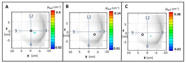
Iso-surface plots of the reconstructed μaxf values for the in vivo reconstruction using experimental data for (A) Case #6, where a 0.45 cm3 (0.95 cm diameter) fluorescent target was placed at approximately the 6 o’clock position, (B) Case #7, where a 0.45 cm3 (0.95 cm diameter) fluorescent target was placed at approximately the 4 o’clock position, and (C) Case #8, where a smaller 0.23 cm3 (0.76 cm diameter) fluorescent target was placed at approximately the 8 o’clock position. The black circle represents the estimated true target location that was placed with respect to the clock positions (shown by the dashed cross-wire).
Figures 10-12 show contour slices in the coronal, sagittal and transverse views for the experimental Cases #6-8, respectively. There was no threshold applied to the contour slices in Figures 10-12. The cutoff was only used in the iso-surface plots (Figures 7-9). The slices for Cases #6-7 (Figures 10-11, respectively) show that a target was recovered apart from the background with a single artifact (reconstructed μaxf that is located away from the estimated target location) also present in each case. For Case #6 (Figure 10) the target is seen in coronal slices where (depth) x=0.5 to 2.0 cm, sagittal slices where y= -1.5 to -2.5 cm, and transverse slices where z= -0.5 to -1.5 cm. The artifact can be seen in coronal slices x=2.0 to 2.5 cm and transverse slice z= -2.5 cm. For Case #7 (Figure 11) the target is seen in coronal slices where x= 3.25 to 3.75 cm, sagittal slices where y=-5.75 to -6.25 cm, and transverse slices where z=0.15 to -0.45 cm. The artifact can be seen in coronal slices x=1.75 to 2.25 cm and transverse slice z=-2.0 to -3.5 cm. For Case #8 (Figure 12) the target is seen in coronal slices where x= 0.6 to 1.5 cm, sagittal slices where y=-1.3 to - 1.9 cm, and transverse slices where z= -1.5 to -2.1 cm. The slices for Case #8 (Figure 12) show that a single target was recovered without artifacts, although it was far from the estimated true location (4.45 cm away). The “true target locations” are only given as estimated clock positions and some shifting of the targets may have occurred as the probe was placed onto the tissue during imaging. Additionally, the accuracy of coregistration is low (~1 cm error) which also may contribute to error in the recovered target location. However, in all cases a distinct target was recovered apart from the background which demonstrates the potential for 3D tomographic imaging in vivo.
Figure 10.
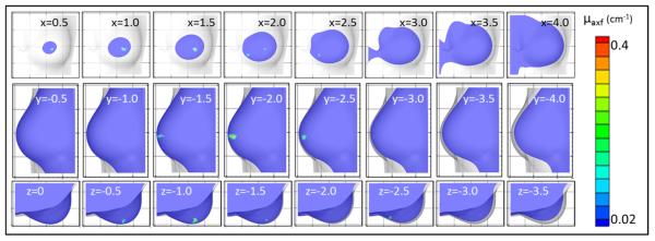
Contour slices in coronal (top row), sagittal (middle row), and transverse (bottom row) views of the reconstructed μaxf values for the in vivo reconstruction using experimental data for Case #6, where a 0.45 cm3 (0.95 cm diameter) fluorescent target was placed at approximately the 6 o’clock position. The coordinate location of each slice is given in cm.
Figure 12.

Contour slices in coronal (top row), sagittal (middle row), and transverse (bottom row) views of the reconstrcuted μaxf values for the in vivo reconstruction using experimental data for Case #8, where a 0.23 cm3 (0.76 cm diameter) fluorescent target was placed at approximately the 8 o’clock position. The coordinate location of each slice is given in cm.
Figure 11.

Contour slices in coronal (top row), sagittal (middle row), and transverse (bottom row) views of the reconstructed μaxf values for the in vivo reconstruction using experimental data for Case #7, where a 0.45 cm3 (0.95 cm diameter) fluorescent target was placed at approximately the 4 o’clock position. The coordinate location of each slice is given in cm.
4. Discussion
Sources of error during real-time 3D positional tracking include instability of the tracker, movement of the subject, and distortion of the breast tissue during compression. Additional error can occur due to the coarseness of the 3D volume mesh in that the nodes may not directly correspond to the spacing of the sources and detectors on the probe face. The coregistered location for each source or detector is limited by the element size (0.5 cm in this case), and the closest node to each source/detector in the probe is assigned as the source/detector node in the mesh. For a coarse mesh this can lead to inaccuracy in the source-detector locations if the true locations are between the mesh nodes. As described in section 3.1, the error in tracking in vivo is about 1 cm using the acoustic tracker. Currently a custom-developed optical tracking system is developed, which had demonstrated improved accuracy (from 11% average error to 6.8% average error) in coregistered imaging of phantoms (Martinez 2010). For future in vivo studies, a second tracker will be added to the subject to account for any movement of the subject during imaging, except for breast distortions (if any) during imaging. A mechanical arm will also be implemented to eliminate movement of the probe by the operator. Breast distortions would be minimized by avoiding compression of the tissue as well as using tissue conforming garments during imaging.
The results for the 3D reconstructions using simulated data in human breast tissue geometry show that a single target was reconstructed close to its true location (1 cm average total distance off) in all five cases. The total distance off (given in Table 2) was 1.59 cm for the first case. The error is mostly in the x-dimension representing the depth in the tissue. The recovered target was located shallower than the true target location. This is due to the physics of reflectance imaging and has been observed by other researchers (Godavarty 2004, Joshi 2006, Kepshire 2007). This can possibly be overcome by acquiring and employing images collected from multiple projections and different locations during tomographic imaging (Ge 2010) or performing transmission measurements-based tomographic imaging. The case of multiple projections has been demonstrated in tissue phantoms where images were collected on two sides of the phantom at 90° angles. One surface image provided the estimated 2D target location and the other surface image provided the estimated depth location. The combined information was then used to give an a priori estimation of the 3D target location. This information was in turn used during image reconstructions, thus improving the target depth recovery (Ge 2010). Additionally, transmission imaging is currently implemented with the hand-held imager, which can potentially improve the depth localization. The tumor to background ratio (T:B) in simulation Cases #1-3 was taken as perfect uptake (1:0) to mimic the current experimental cases (where ICG was in the target and not injected into the breast tissue). The recovered T:B ratios (Table 2) were relatively high ~200:1, which closely corresponds to perfect uptake. The simulation Cases #4-5 were performed to model the case of imperfect uptake (using T:B of 100:1 and 50:1, respectively). At this feasibility stage a higher T:B was chosen initially. Extensive studies will be performed in the future to determine the lowest T:B ratio, smallest sized target, etc. that can be recovered using the hand-held optical imager. Additionally, the actual T:B ratios in human subject was not available as observed from past research (Corlu 2007, Sevick-Muraca 2008) in order to determine if the 100:1 and 50:1 ratios of ICG are typical for breast imaging. A single target was reconstructed in each case yet the recovered T:B ratios were very low (6:1 and 1:1, respectively). For true in vivo studies, an image from the contralateral breast can be used to subtract and remove the background noise as well as the background fluorescence. The simulation cases presented here do not reflect any post-process subtraction to remove or reduce background fluorescence.
The results for the 3D reconstructions using experimental data (cases #6-8) with a fluorescent target placed under the inframammary fold of the breast tissue in a human subject show that the targets were recovered, although farther from the estimated target location than in the simulated cases, which is likely due to movement of the target during placement and/or imaging. From the experimental results in Figures 10-12 (Cases #6-8) it can also be seen that the recovered targets’ distance from the curved tissue surface is shallower than the true target location. For in vivo cases, the shallow target recovery might be attributed to the compression of the tissue (in addition to the physics of reflectance-based measurements) during imaging which is not reflected in the scanned tissue geometry. The tissue conforming garment currently being developed will prevent the breast tissue from moving or deforming during imaging allowing the scanned geometry to remain constant. Additionally, some groups have shown that spectral approaches may improve tumor localization in DOT reconstructions (Corlu 2003, Srinivasan 2005, selected references). The recovered target volume is almost double the true target volume in all three experimental (as well as simulated) cases which is likely due to the coarseness of the discretized mesh that was generated for reduced computational time. More refined discretization may improve the volume and shape of the recovered targets (which is yet to be tested). The recovered target volume and T:B ratio for Case #6 (experimental data under perfect uptake) show results comparable to the simulation cases #1- 3; however, for Case #7 (experimental data under perfect uptake) the values are low. The x,y,z values given as the approximate true target location are a very rough estimate based on the intended placement of the target at the 6 o’clock, 4 o’clock, and 8 o’clock positions. The target was placed visually under the tissue and could possibly have moved as the tissue was compressed by the probe. In a true case of breast cancer imaging, the target location would be better estimated from the medical records (e.g. x-ray mammography, ultrasound) in order to assess the ability to recover a tumor at its true location in vivo. The artifacts that appear in the reconstructed images for Case #6 and #7 (Figures 10 and 11) are likely due to movement of the probe and the breast tissue during removal of the target. Differences between the target and background images will appear as noise, or artifacts, in the subtracted image. Currently post-processing methods are explored in efforts to reduce the artifacts.
The current goal for this initial study was to demonstrate the feasibility of performing 3D tomography using our hand-held imager. Currently diffuse optical imaging studies (without external contrast) are performed in breast cancer patients to determine the ability of the device to detect breast tumors in real-time as 2D surface images, based on the endogenous contrast even prior to injection of a fluorescent contrast agent. The 2D surface optical images of in vivo breast cancer show promise (manuscript in preparation) in that we have been able to detect tumors upon endogenous contrast (even without the use of fluorescence contrast agents). Future work will involve performing 3D tomographic imaging on breast cancer subjects, during which the extent to recover small and deep targets will be determined.
5. Conclusion
A hand-held optical imager has been developed and its capability to perform 3D tomographic imaging via coregistration facilities is demonstrated. Coregistered imaging was validated in vivo and real-time coregistered images were used to perform 3D reconstructions of fluorescent targets in healthy breast tissue of a human subject. The results show the feasibility of performing 3D tomographic imaging and of breast tissues and 3D localization of fluorescent target(s) (superficially placed under the breast fold) using a hand-held optical imager.
Acknowledgments
This work was supported by the Department of Defense (BC083282), the American Cancer Society and Canary Foundation (121585-PFTED-11-219-01-SIED), NIH (R15-CA119253), and Coulter Early Career Translational Grant.
References
- Alacam B, Yazici B, Intes X, Nioka S, Chance B. Pharmacokinetic-rate images of indocyanine green for breast tumors using near-infrared optical methods. Phys. Med. Biol. 2008;53:837–859. doi: 10.1088/0031-9155/53/4/002. [DOI] [PubMed] [Google Scholar]
- Cerussi A, Shah N, Hsiang D, Durkin A, Butler J, Tromberg BJ. In vivo absorption, scattering, and physiologic properties of 58 malignant breast tumors determined by broadband diffuse optical spectroscopy. J. Biomed. Opt. 2006;11(4):044005. doi: 10.1117/1.2337546. [DOI] [PubMed] [Google Scholar]
- Cerussi A, Hsiang D, Shah N, Mehta R, Durkin A, Butler J, Tromberg BJ. Predicting response to breast cancer neoadjuvant chemotherapy using diffuse optical spectroscopy. Proc. Natl. Acad. Sci., USA. 2007;104(10):4014–4019. doi: 10.1073/pnas.0611058104. [DOI] [PMC free article] [PubMed] [Google Scholar]
- Chance B, Nioka S, Conant EF, Hwang E, Briest S, Orel SG, Schnall MD, Czerniecki BJ. Breast cancer detection based on incremental biochemical and physiological properties of breast cancers: A six-year, two-site study. Acad. Radiol. 2005;12(8):925–933. doi: 10.1016/j.acra.2005.04.016. [DOI] [PubMed] [Google Scholar]
- Choe R, et al. Diffuse optical tomography of breast cancer during neoadjuvant chemotherapy: a case study with comparison to MRI. Med. Phys. 2005;32:1128–1139. doi: 10.1118/1.1869612. [DOI] [PubMed] [Google Scholar]
- Choe R, et al. Differentiation of benign and malignant breast tumors by in-vivo three-dimensional parallel-plate diffuse optical tomography. J Biomed Opt. 2009;14(2):024020. doi: 10.1117/1.3103325. [DOI] [PMC free article] [PubMed] [Google Scholar]
- Corlu A, Durduran T, Choe R, Schweiger M, Hillman EM, Arridge SR, Yodh AG. Uniqueness and wavelength optimization in continuous-wave multispectral diffuse optical tomography. Opt. Lett. 2003;28(23):2339–2341. doi: 10.1364/ol.28.002339. [DOI] [PubMed] [Google Scholar]
- Corlu A, Choe R, Durduran T, Rosen MA, Schweiger M, Arridge SR, Schnall MD, Yodh AG. Three-dimensional in vivo fluorescence diffuse optical tomography of breast cancer in humans. Optics Express. 2007;15(11):6696–6716. doi: 10.1364/oe.15.006696. [DOI] [PubMed] [Google Scholar]
- Culver JP, Choe R, Holboke MJ, Zubkov L, Durduran T, Slemp A, Ntziachristos V, Pattanayak DN, Chance B, Yodh AG. 3D diffuse optical tomography in the plane parallel transmission geometry: Evaluation of a hybrid frequency domain/continuous wave clinical system for breast imaging. Med. Phys. 2003;30:235–247. doi: 10.1118/1.1534109. [DOI] [PubMed] [Google Scholar]
- Erickson SJ, Godavarty A. Hand-Held Based Near-Infrared Optical Imaging Systems: A Review. Med. Eng. and Phys. 2009;31:495–509. doi: 10.1016/j.medengphy.2008.10.004. [DOI] [PubMed] [Google Scholar]
- Erickson SJ, Ge J, Sanchez A, Godavarty A. Two-dimensional fast surface imaging using a hand-held optical device: in-vitro and in-vivo fluorescence studies. Trans. Oncol. 2010a;3(1):16–22. doi: 10.1593/tlo.09157. [DOI] [PMC free article] [PubMed] [Google Scholar]
- Erickson SJ, Martinez S, DeCerce J, Romero A, Caldera L, Godavarty A. In: Vo-Dinh Tuan, Grundfest Warren S., Mahadevan-Jansen Anita., editors. Fast coregistered imaging in vivo using a hand-held optical imager Advanced Biomedical and Clinical Diagnostic Systems VIII; Proceedings of the SPIE.2010b. pp. 75550P–75550P-6. [Google Scholar]
- Erickson SJ, Godavarty A, Martinez SL, Gonzalez J, Romero A, Roman M, Nunez A, Ge J, Regalado S, Kiszonas R, Lopez-Penalver C. Hand-held optical devices for breast cancer: spectroscopy and tomographic imaging. IEEE JSTQE. 2012;18(4):1298–1312. [Google Scholar]
- Fedele F, Laible JP, Eppstein MJ. Coupled complex adjoint sensitivities for frequency-domain fluorescence tomography: Theory and vectorized implementation. J. Comput. Phys. 2003;187(2):597–619. [Google Scholar]
- Ge J, Zhu B, Regalado S, Godavarty A. Three-dimensional fluorescence-enhanced optical tomography using a hand-held probe based imaging system. Med. Phys. 2008;35(7):3354–3363. doi: 10.1118/1.2940603. [DOI] [PMC free article] [PubMed] [Google Scholar]
- Ge J, Erickson SJ, Godavarty A. Multi-projection fluorescence optical tomography using a handheld-probe-based optical imager: phantom studies. Applied Optics. 2010;49:4343–4354. doi: 10.1364/AO.49.004343. [DOI] [PMC free article] [PubMed] [Google Scholar]
- Godavarty A, Eppstein MJ, Zhang C, Theru S, Thompson AB, Gurfinkel M, Sevick-Muraca EM. Fluorescence-enhanced optical imaging in large tissue volumes using a gain modulated ICCD camera. Phys. Med. Biol. 2003;48:1701–1720. doi: 10.1088/0031-9155/48/12/303. [DOI] [PubMed] [Google Scholar]
- Godavarty A, Zhang C, Eppstein MJ, Sevick-Muraca EM. Fluorescence-enhanced optical imaging of large phantoms using single and simultaneous dual point illumination geometries. Med. Phys. 2004;31:183–90. doi: 10.1118/1.1639321. [DOI] [PubMed] [Google Scholar]
- Grosenick D, Moesta KT, Wabnitz H, Mucke J, Stroszczynski C, MacDonald R, Schlag PM, Rinneberg H. Timedomain optical mammography: Initial clinical results on detection and characterization of breast tumors. Appl. Opt. 2003;42:3170–3186. doi: 10.1364/ao.42.003170. [DOI] [PubMed] [Google Scholar]
- Grosenick D, Moesta KT, Möller M, Mucke J, Wabnitz H, Gebauer B, Stroszczynski C, Wassermann B, Schlag PM, Rinneberg H. Time-domain scanning optical mammography: I. Recording and assessment of mammograms of 154 patients. Phys. Med. Biol. 2005;50:2429–2449. doi: 10.1088/0031-9155/50/11/001. [DOI] [PubMed] [Google Scholar]
- Jayachandran B, Ge J, Regalado S, Godavarty A. Design and development of a hand-held optical probe toward fluorescence diagnostic imaging. J Biomed Opt. 2007;12(5):054014. doi: 10.1117/1.2799193. [DOI] [PubMed] [Google Scholar]
- Joshi A, Bangerth W, Hwang K, Rasmussen JC, Sevick-Muraca EM. Fully adaptive FEM based fluorescence optical tomography from time-dependent measurements with area illumination and detection. Med. Phys. 2006;33(5):1299–1310. doi: 10.1118/1.2190330. [DOI] [PubMed] [Google Scholar]
- Kepshire DS, Davis SC, Dehghani H, Paulsen KD, Pogue BW. Subsurface diffuse optical tomography can localize absorber and fluorescent objects but recovered image sensitivity is nonlinear with depth. Appl. Opt. 2007;46(10):1669–1678. doi: 10.1364/ao.46.001669. [DOI] [PubMed] [Google Scholar]
- Kogure K, David NJ, Yamanouchi U, Choromokos E. Infrared absorption angiography of the fundus circulation. Arch. Ophthalmol. 1970;83(2):209–214. doi: 10.1001/archopht.1970.00990030211015. [DOI] [PubMed] [Google Scholar]
- Leff DR, Warren OJ, Enfield LC, Gibson A, Athanasiou T, Patten DK, Hebden J, Yang GZ, Darzi A. Diffuse optical imaging of the healthy and diseased breast: A systematic review. Breast Cancer Res Treat. 2008;108:9–22. doi: 10.1007/s10549-007-9582-z. [DOI] [PubMed] [Google Scholar]
- Leevy CM, Smith F, Longueville J. Indocyanine green clearance as a test for hepatic function: evaluation by dichromatic ear densitometry. J. Am. Med. Assoc. 1967;200:236–240. [PubMed] [Google Scholar]
- Martinez S, DeCerce J, Gonzalez J, Erickson SJ, Godavarty A. Biomedical Optics, OSA Technical Digest. Optical Society of America; 2010. Assessment of Tracking Devices towards Accurate Coregistration in a Hand-Held Optical Imager. 2010), paper BTuD58. [Google Scholar]
- Nioka S, Yung Y, Schnall M, Zhao S, Orel S, Xie C, Chance B, Solin S. Optical imaging of breast tumor by means of continuous waves. Adv. Exp. Med. Biol. 1997;411:227–32. doi: 10.1007/978-1-4615-5865-1_27. [DOI] [PubMed] [Google Scholar]
- Poellinger A, Marti JC, Ponder SL, Freund T, Hamm B, Bick U, Diekmann F. Near-infrared Laser Computed Tomography of the Breast: First Clinical Experience. Acad Radiol. 2008;15:1545–1553. doi: 10.1016/j.acra.2008.07.023. [DOI] [PubMed] [Google Scholar]
- Rasmussen JC, Tan I-C, Marshall MV, Fife CE, Sevick-Muraca EM. Lymphatic imaging in human with near-infrared fluorescence. Current Opinion in Biotechnology. 2009;20(1):74–82. doi: 10.1016/j.copbio.2009.01.009. [DOI] [PMC free article] [PubMed] [Google Scholar]
- Regalado S, Erickson SJ, Zhu B, Ge J, Godavarty A. Automated coregistered imaging using a hand-held probe-based optical imager. Rev. Sci. Inst. 2010;81:023702. doi: 10.1063/1.3271019. [DOI] [PubMed] [Google Scholar]
- Sevick-Muraca EM, et al. Imaging of lymph flow in breast cancer patients after microdose administration of near-infrared fluorophore: feasibility study. Radiology. 2008;246(3):734–41. doi: 10.1148/radiol.2463070962. [DOI] [PMC free article] [PubMed] [Google Scholar]
- Srinivasan S, Pogue BW, Jiang S, Dehghani H, Paulsen KD. Spectrally constrained chromophore and scattering near-infrared tomography provides quantitative and robust reconstruction. Appl. Opt. 2005;44(10):1858–1869. doi: 10.1364/ao.44.001858. [DOI] [PubMed] [Google Scholar]
- Taroni P, Torricelli A, Spinelli L, Pifferi A, Arpaia F, Danesini G, Cubeddu R. Time-resolved optical mammography between 637 and 985 nm: Clinical study on the detection and identification of breast lesions. Phys. Med. Biol. 2005a;50:2469–2488. doi: 10.1088/0031-9155/50/11/003. [DOI] [PubMed] [Google Scholar]
- Taroni P, Spinelli L, Torricelli A, Pifferi A, Danesini GM, Cubeddu R. Multi-wavelength time domain optical mammography. Tech. Cancer Res. Treat. 2005b;4:527–537. doi: 10.1177/153303460500400506. [DOI] [PubMed] [Google Scholar]
- Taroni P, Pifferi A, Quarto G, Spinelli L, Torricelli A, Abbate F, Villa A, Balestreri N, Menna S, Cassano E, Cubeddu R. Non-invasive assessment of breast cancer risk using time-resolved diffuse optical spectroscopy. J. Biomed. Opt. 2010;15:060501. doi: 10.1117/1.3506043. [DOI] [PubMed] [Google Scholar]
- Tromberg BJ, Coquoz O, Fishkin JB, Pham T, Anderson ER, Butler J, Cahn M, Gross JD, Venugopalan V, Pham D. Non-invasive measurements of breast tissue optical properties using frequency-domain photon migration. Philos. Trans. R Soc. Lond. B Biol. Sci. 1997;352:661–668. doi: 10.1098/rstb.1997.0047. [DOI] [PMC free article] [PubMed] [Google Scholar]
- Van de Ven SMWY, et al. Diffuse optical tomography of the breast: initial validation in benign cysts. Mol Imaging Biol. 2009a;11:64–70. doi: 10.1007/s11307-008-0176-x. [DOI] [PMC free article] [PubMed] [Google Scholar]
- Van de Ven SMYW, et al. Diffuse Optical Tomography of the Breast: Preliminary Findings of a New Prototype and Comparison with Magnetic Resonance Imaging. Eur Radiol. 2009b;19(5):1108–1113. doi: 10.1007/s00330-008-1268-3. [DOI] [PubMed] [Google Scholar]
- Van de Ven SMWY, et al. A Novel Fluorescent Imaging Agent for Diffuse Optical Tomography of the Breast: First Clinical Experience in Patients. Mol Imaging Biol. 2010;12:343–348. doi: 10.1007/s11307-009-0269-1. [DOI] [PMC free article] [PubMed] [Google Scholar]