Abstract
Compensating for the collimator-detector response (CDR) in SPECT is important for accurate quantification. The CDR consists of both a geometric response and a septal penetration and collimator scatter response. The geometric response can be modeled analytically and is often used for modeling the whole CDR if the geometric response dominates. However, for radionuclides that emit medium or high-energy photons such as I-131, the septal penetration and collimator scatter response is significant and its modeling in the CDR correction is important for accurate quantification. There are two main methods for modeling the depth-dependent CDR so as to include both the geometric response and the septal penetration and collimator scatter response. One is to fit a Gaussian plus exponential function that is rotationally invariant to the measured point source response at several source-detector distances. However, a rotationally-invariant exponential function cannot represent the star-shaped septal penetration tails in detail. Another is to perform Monte-Carlo (MC) simulations to generate the depth-dependent point spread functions (PSFs) for all necessary distances. However, MC simulations, which require careful modeling of the SPECT detector components, can be challenging and accurate results may not be available for all of the different SPECT scanners in clinics. In this paper, we propose an alternative approach to CDR modeling. We use a Gaussian function plus a 2-D B-spline PSF template and fit the model to measurements of an I-131 point source at several distances. The proposed PSF-template-based approach is nearly non-parametric, captures the characteristics of the septal penetration tails, and minimizes the difference between the fitted and measured CDR at the distances of interest. The new model is applied to I-131 SPECT reconstructions of experimental phantom measurements, a patient study, and a MC patient simulation study employing the XCAT phantom. The proposed model yields up to a 16.5 and 10.8% higher recovery coefficient compared to the results with the conventional Gaussian model and the Gaussian plus exponential model, respectively.
Index Terms: B-spline point spread function template, collimator-detector response, I-131 quantitative SPECT
I. Introduction
Accurate quantification in single photon emission computed tomography (SPECT) is important in many applications. For example, accurate SPECT-based dosimetry in internal emitter therapies such as I-131 radioimmunotherapy and radioiodine therapy can potentially improve dose-response correlations so that the efficacy and toxicity of the treatments can be better assessed. There has been considerable research on improving the quantitative accuracy in SPECT by using various correction methods: attenuation correction, object scatter correction, and collimator-detector response (CDR) compensation [1]–[6].
The CDR, which consists of both a geometric component and a septal penetration and collimator scatter component, is one of the most important degrading factors in quantitative SPECT imaging. Incorporating depth-dependent CDRs in the system matrix of an iterative image reconstruction improves performance [5]. The septal penetration and collimator scatter component is particularly problematic for radionuclides that emit medium or high-energy photons [7]–[11]. The geometric response can easily be modeled analytically, whereas modeling the septal penetration and collimator scatter response is more challenging. Up to now, three main approaches have been used.
The first approach is to model only the geometric response and to ignore the septal penetration and collimator scatter response. One can analytically calculate the geometric transfer function by using the scanner parameters (e.g., collimator specifications and distance between detector and imaging plane) [12], [13]. This approach is easy to use and works well when the geometric response dominates the CDR (e.g., for Tc-99m). It is used for CDR modeling in most commercial iterative reconstruction software available with SPECT systems due to its simplicity. The geometric component can be well fitted with a Gaussian function [13]. However, this model does not consider the septal penetration and collimator scatter response.
-
The second approach is to use Monte-Carlo (MC) simulation techniques. One can either generate a table of the depth-dependent CDR functions using MC simulation [2], [3], [8], [10], or use a MC simulator itself as a forward projector in an iterative image reconstruction [14]. With this approach it is possible to model all components of the CDR including the septal penetration and collimator scatter response, which is important for accurate quantitative SPECT with radionuclides that emit medium or high-energy photons such as I-131, In-111, Ga-67, and I-123.
However, MC simulations that include the septal penetration and collimator scatter response are challenging and accurate results may not be available for all of the different SPECT scanners in clinics. Even though generating a table of depth-dependent CDRs with very low noise requires their computation only once, it is still computationally demanding [2]. There have been some efforts to develop faster MC simulations that include the septal penetration and collimator scatter response [9], [11], [15], but using a MC simulator as a forward projector involves high computational complexity [14]. In addition, one should validate the MC simulation by comparison of simulated energy spectra and PSFs with experimental measurements. For higher-energy photons it has been shown that it is important to carefully model all components of the SPECT detector system (collimator, back compartment, shielding) to get good agreement between measurement and simulation [9], [16], [17]. Even small discrepancies between collimator specification provided by the manufacturer and the actual dimensions of the collimator can lead to significant mismatch between measurement and simulation.
Lastly, one can use point source measurements from a scanner for CDR modeling. The point source should be measured at many locations for both a SPECT system with rotating detectors [18] and a stationary SPECT system [19], [20]. However, for the former case, the number of required measurements is usually smaller: by assumption, one needs only to place the point source at several source-to-detector distances while keeping the rotation angle fixed. For conventional SPECT systems with rotating detectors, one can fit a 2-D function such as a Gaussian function to the measured point source at several distances and then use the fit results to produce a model of the depth-dependent CDR. Since a Gaussian function cannot describe the septal penetration and collimator scatter response, a 2-D Gaussian plus a heavy-tailed function such as an exponential have been used to fit the measurements [6], [18]. Usually, the Gaussian function fits the geometric component of the CDR and the exponential function fits the septal penetration and collimator scatter response component. However, a rotationally-invariant exponential function cannot represent the “star-shaped” septal penetration tails of the CDR in detail (see Fig. 1).
Fig. 1.
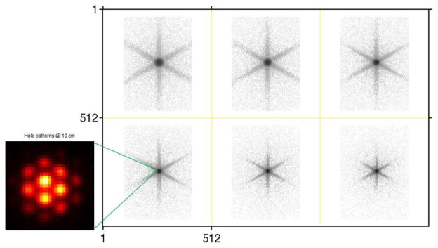
Measured I-131 point source images at six different distances between the front surface of the collimator and the object plane. Top row: 25, 20, 15 cm, bottom row: 10, 5, 2 cm. Zoomed point source image at 10 cm shows hole pattern due to high-energy collimator. The image intensity is presented on a logarithmic grey scale except for the zoomed image.
In this paper, we focus on this last approach and use point source measurements from a conventional SPECT system with rotating detectors. However, we propose a “nearly non-parametric” model of the CDR (a 2-D Gaussian function plus a point spread function (PSF) template) and fit the proposed model to the measured point source response at six different distances. This approach is intended to provide an alternative to the MC simulation technique. It is most appropriate when accurate MC simulations are not available for a given SPECT scanner. By better fitting the septal penetration tails, our approach is designed to increase quantification accuracy for radionuclides that emit medium or high-energy photons compared to that using Gaussian or Gaussian plus exponential functions.
Section II reviews how to model the depth-dependent CDR by using function fitting. Section III details the PSF template approach that uses B-spline PSF templates. Sections IV and V present the results of our proposed approach. The results will show improved CDR model fitting to the point source measurements compared with previous approaches using fitting by the Gaussian function and by the Gaussian plus exponential function. In addition, image reconstruction results for experimental and digital phantom studies will show improvements in quantification with our method.
II. Function Fitting Approach for CDR Modeling
In this section, we review procedures for the “function fitting approach” of modeling the depth-dependent CDR using point source measurements at several distances [18].
A. Gaussian Function Fitting Approach
Here, we describe using a Gaussian function to fit the measured point source CDRs. However, the procedure can be applied to other parametric functions.
Suppose that we obtained several point source measurements pm at several source-to-detector distances dm where m = 1, …M. We assume that pm is scatter-corrected for each m (e.g., using a triple energy window (TEW) method [21]) because usually object-specific scatter correction, which will include collimator scatter, is applied separately during our reconstruction procedure.
The following two steps are used to obtain a normalized CDR (or PSF) as a function of distance.
The first step is to fit a discretized version of a 2-D Gaussian function
| (1) |
to each pm. In other words, the amplitude a1,m and the width w1,m for each distance dm are estimated by
| (2) |
where (xj, yj) is the discretized location of the jth pixel in pm. One can use any nonlinear least square fitting for (2) [22]. In this first function fitting, we obtain the amplitude â1,m and the width ŵ1,m for all distances dm, m = 1, …, M.
The second step is to fit a 1-D function of distance d to the amplitude â1,m and the width ŵ1,m. One can use any 1-D function-fitting tool to find good functions of d to fit all M values of â1,m and ŵ1,m. We chose the following functions for the amplitude a1 (d) and the width w1 (d):
| (3) |
| (4) |
where b5 and b6 are nonnegative. One can obtain the estimates of bi, i = 1, … 7 by fitting a1 (d; b1, b2, b3, b4) and w1 (d; b5, b6, b7) to the amplitude â1,m and the width ŵ1,m, respectively.
Therefore, from these two steps, one can model the depth-dependent PSF at a distance d by plugging (3) and (4) into (1) as follows:
| (5) |
where Z(d) is a normalization factor such that ∫ ∫ PSFG(x; y; d) dx dy = 1. Using (5), one can generate samples of the (normalized) Gaussian CDR at any distance. Finding a1 (d) is redundant for this Gaussian case due to the normalization factor Z(d), but it will be necessary for the next two cases.
B. Gaussian + Exponential Function Fitting Approach
The CDR model (5) using a 2-D Gaussian function is well suited for describing the geometric component of the CDR, but cannot capture the details of the septal penetration tails. Modeling the septal penetration is important for accurate quantification in SPECT imaging with radionuclides that emit medium or high-energy photons such as I-131. Koral et al. used the sum of a 2-D Gaussian plus exponential function instead of (1) for modeling the CDR as follows [18]:
| (6) |
for each distance dm where fG is defined in (1). We use the same procedure in Section II-A to derive a PSFGE (x, y; d) that better fits the measurements pm than (5).
This Gaussian plus exponential function model (6) is circularly symmetric unlike the star-shaped penetration tails (see Fig. 1). This mismatch between the model and the data suggests that we should be able to improve the fit further by using other functions.
III. B-Spline PSF Template Approach
This section describes the B-spline PSF template model that can potentially improve the CDR fit to the point source measurements compared to that with either (1) or (6).
A. B-Spline PSF Template
To describe the rotationally-variant, star-shaped penetration tails of the CDR better, we propose using the following 2-D B-spline PSF template instead of the exponential function underlying (6):
| (7) |
where cik are B-spline coefficients, i, k are integers, β is a B-spline basis and hx, hy denote the B-spline knot spacing between the centers of the adjacent B-spline bases. We hypothesize that the CDR has a common shape at all source-to-detector distances and, furthermore, assume that (7), by appropriate spatial scaling, can yield a good fit to the point source measurements obtained at different distances.
By using this B-spline template (7), we propose to use the following CDR model instead of (6):
| (8) |
for each distance dm. The B-spline coefficients cik do not depend on the distance dm and they describe the common shape. We estimate the shape of the PSF template (the measurement minus the Gaussian fit) using all the measurements at all distances at the same time. Therefore, separate optimization of (2) for each distance dm is not applicable to this new CDR model. We will present a new cost function and an optimization scheme for the new CDR model in Section III-B and III-C.
We represent a discretized version of (7) by a simple matrix form as follows:
| (9) |
where c is a vector with the elements {cik} and B is a matrix with the elements [B]j,ik = β(xj/hx − i)β(yj/hy − k). In this case, a discretized version of (8) can also be represented as follows:
| (10) |
where
and
Both Tshift and Tscale can be implemented with any image interpolation method. We used a cubic B-spline interpolation to implement these matrices [23]. Smaller hx, hy can potentially improve the fitting of (10) to the measurements due to the greater number of degrees of freedom, but the increased number of parameters to estimate would make the nonlinear, nonconvex optimization problem more ill-posed. Considering this trade-off, we chose hx = hy = 4 pixels in our implementation.
B. Cost Function for Spatially-Invariant PSF Template
Any spatial variations in the hole pattern at a given distance dm are usually ignored in SPECT image reconstruction in order to calculate the CDR in the system matrix more efficiently (e.g., using the fast Fourier transform). Both (1) and (6) are space-invariant PSF models because they ignore the details of the hole pattern (see Fig. 1 for a hole pattern example). In the MC simulations, the CDRs at different spatial locations of the source that had the same source-to-detector distance were averaged.
Due to its considerable flexibility, our proposed PSF template can potentially describe the spatially-variant hole pattern, but doing so is inconsistent with efficient image reconstruction. Therefore, we designed the cost function to produce a spatially-invariant CDR estimate.
Since we searched for the common shape of a B-spline PSF template for all measured distances, we effectively averaged the hole patterns of the CDR from several source-to-detector distances. However, it was still possible to have some spatially-variant hole patterns in the PSF template estimate. So, we postulated the following three properties of the CDR and required their fulfillment for the estimate of the PSF template (8) so that the hole patterns were suppressed more completely.
First, the CDR is smooth. Even though the B-spline itself is a smooth basis, we also penalized the roughness of the PSF template to further control the smoothness. Second, the CDR is symmetric. Due to the geometry of the hexagonal collimator that we used, the CDR should be the same for any number of 60° rotations. (For foil collimators with four penetration tails, left–right and top–bottom symmetry could be used instead.) Third, the CDR is nonnegative. This requirement followed from the fact that the normalized CDR represents a detection probability and that a probability cannot be negative.
Thus, we used the following cost function with three priors:
| (11) |
where uq is the location of the point source measurement (q = x, y), ηl’s are regularization parameters (l = 1, 2, 3), and pl’s are regularizers for smooth, symmetric, and nonnegative properties of the CDR (l = 1, 2, 3). We set the amplitude an, round(M/2) ≜ 1 and the width wn, round(M/2) ≜ 1. The first regularizer p1 is defined as
where C is a first-order difference matrix (x and y directions). The second regularizer p2 is described as follows:
where
and
Lastly, the third regularizer p3 is simply where x− ≜ x for x < 0 and x− ≜ 0 for x ≥ 0. We determined the regularization parameters empirically so that the estimated PSF template showed the three assumed properties of the CDR with the following results: η1 = 1, η2 = 103, and η3 = 10.
C. Optimization for B-Spline PSF Template
One can use any optimization algorithm to minimize (11). We chose to use block alternating minimization. We repeated two minimization steps: one minimization with respect to the Gaussian function fG and the other minimization with respect to the B-spline PSF template bB. Although both fG and bB contain variables ux and uy, we treated them separately.
We used a nonlinear least square algorithm [22] for minimizing (11) with respect to the Gaussian function
| (12) |
which is the same minimization method we used to estimate the parameters for the Gaussian PSF model (1) and the Gaussian plus exponential PSF model (6). We minimized (11) with respect to the B-spline PSF template as follows:
| (13) |
| (14) |
using the L-BFGS [24] algorithm. We performed (12), (13), and (14) in order, and repeated the process several times.
Once we obtained all parameters from the above minimization, we fit the amplitude an,m and wn,m the width (scaling) to the functions in (3) and (4), respectively. Thereby, we finally obtained the desired PSFGB (x, y; d) function.
IV. Evaluation
We performed all of our I-131 studies with the Siemens Symbia TruePoint SPECT-CT using high-energy collimation for the dual heads. The studies employed both experimental measurements and simulations with the SIMIND (Simulation of Imaging Nuclear Detection) MC simulator [25]. The shape of the high-energy collimators was hexagonal with a septal thickness of 2 mm, a hole diameter of 4 mm, and a hole length of 59.7 mm. The system resolution at 10 cm was 13.4 mm. Using the TEW method, an object scatter correction was applied to the point source measurements, and an object scatter estimate was employed in the phantom reconstructions and in the patient reconstructions. The main window for the TEW correction was set at 20% (centerline 364 keV) and the two adjacent subwindows were set at 6% (subwindow centerlines at 318 and 413 keV, respectively) [21].
A. Measurement of Point Source at Several Distances
We measured the CDR at several distances between the front surface of the collimator and the object plane. We placed an I-131 point-like source (about 7 mm diameter, 658 μCi) on a Styrofoam cup (low scatter medium) that stood on a flat bed. The source was positioned off the center of the image plane by 11 mm in one direction and 7 mm in the other. We acquired six planar images (512 × 512 bins, 1.2 × 1.2 mm pixels), one each at a distance of 25, 20, 15, 10, 5, and 2 cm. The data were acquired for 20 min per distance.
Fig. 1 shows the measured I-131 point source at the six distances. The image intensity is presented on a logarithmic grey scale to better show the penetration tails [13].
We also simulated our point source (7 mm diameter) measurements at the same six distances using the SIMIND MC simulator and fitted the three CDR models (1), (6), and (8) to the images. To evaluate the goodness of fit, we performed another MC simulation to generate the point source measurements at distances that were different and greater in number (11 instead of six) and generated with a different random seed.
B. Hot Phantom Studies
We performed two separate studies using an elliptical phantom with six spherical lesions. The lesion volumes were 96, 62, 16, 11, 8, and 4 cc. In the first study, the spheres contained I-131 activities in μCi (activity concentration in μCi/cc in parentheses) of 191 (1.99), 121 (1.95), 35 (2.19), 29 (2.64), 29 (3.63), and 29 (7.25), but there was no activity in the background water. In the second study, using the same format, the spheres contained activities of 96 (1.00), 61 (0.98), 18 (1.13), 15 (1.36), 14 (1.75), and 14 (3.50), and the background water contained 2.20 mCi (concentration 0.19 μCi/cc). In the second study, the sphere-to-background concentration ratios were 5.26:1, 5.18:1, 5.92:1, 7.18:1, 9.21:1, and 18.42:1 from largest to smallest sphere. For each study, the individual scan time was 40 min and the acquisition was performed with the SPECT-CT scanner in body-contouring mode. Projection data were acquired at 60 views (angles) of 128 × 128 bins (4.8 × 4.8 mm). Also, CT images were obtained and used to calculate attenuation correction maps. Finally, TEW object scatter estimates were employed during reconstruction. We repeated the scanning for a total of eight realizations in the first study, and for a total of seven realizations in the second.
We generated projections that modeled the depth-dependent normalized CDRs for all projection views and accounted for the changing radius of rotation due to body contouring. We employed the three models: Gaussian PSFG(x, y; d) with (1) (Gaussian), the Gaussian plus exponential PSFGE(x, y; d) with (6) (GauExp), and the Gaussian plus B-spline PSF template PSFGB(x, y; d) with (8) (GauBspl). Then these depth-dependent PSFs were effectively incorporated into the system matrix by convolving the CDR with the projection at each depth. The rotate-sum method using bilinear interpolation for rotating the current estimate of the activity distribution speeds up a CDR compensation routine by using the fast Fourier transform (FFT) [26] and we used that method in our implementation. A 3-D ordered-subset expectation maximization (OSEM) reconstruction with 35 iterations and six subsets, which is the reconstruction used in our patient studies [27], was performed using the CDR-compensated system matrix. The result of the projection using this system matrix produced an estimate of the primary photons and the TEW object scatter estimate was then added. Thus, Poisson statistics were preserved.
The 3-D regions of interest (ROIs) for the six hot spheres were drawn on the CT image and applied to the SPECT reconstruction. We calculated an activity recovery coefficient (RC) from the counts within the ROIs as a quantification measure. The RC of the ROI relative to the field-of-view (FOV) was calculated as
| (15) |
Note that
| (16) |
is the measured activity in the ROI. Thus, (15) becomes the ratio of measured activity to true activity, the standard definition of activity recovery coefficient.
C. Patient Study
We applied our proposed CDR compensation method retrospectively to SPECT-CT data from a patient imaged under an ongoing research protocol for an I-131 radioimmunotherapy dosimetry study [27]. The SPECT data consisted of a 20-min acquisition with body contouring, 60 views, and 128 × 128 bins (4.8 × 4.8 mm), and a low-dose CT acquired for attenuation correction. We applied the TEW object scatter correction to the data and carried out the SPECT image reconstruction with the three different CDR models of Section IV-B.
Patient tumors were delineated on the CT image by a trained Radiologist. Since we did not know the true activity in the ROI and FOV, we set the activity to 1 in (15) so that the count ratio (CR) could be defined as follows:
| (17) |
This CR is directly proportional to the RC since the unknown true activities do not change between the different reconstructions. Thus, any increase of the CR with a given reconstruction implies an increase of the RC with that reconstruction.
D. MC Simulation Study With XCAT Phantom
We also evaluated our proposed method using MC simulated data corresponding to the XCAT phantom [28] and the same SPECT-CT system used in the experimental studies. We simulated the XCAT phantom with five spherical lesions (6, 10, 20, 70, 109 cc) near the liver and kidneys. We set the relative activity concentrations in the XCAT phantom as follows: lesion 100, kidney 80, spleen 51, lung 28, liver 21, and whole body 6. These choices were based on data from a patient [4]. We obtained low noise projection images of the XCAT phantom. We used the same SPECT image reconstruction methods as described in Section IV-B. The reconstructions using the low noise projections produced approximate mean images [29].
The aim of this MC simulation study was to determine the performance improvement with our proposed method for a more realistic geometry than the “hot-sphere” phantom. Thus, we did not use MC-simulation-based CDR compensation, but used the function fitting approach with different models for the simulated point source measurements.
V. Results
A. Fitting CDR Models to Measurements
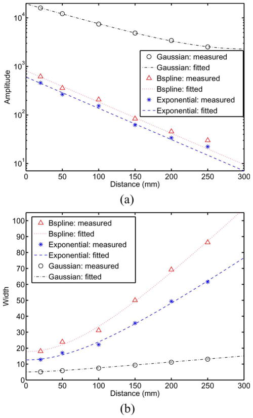
We estimated the amplitudes an,m and widths wn,m to fit the three CDR models (1), (6), and (8) to the point source measurement of Fig. 1 for each distance dm. Points (○, *, ▷) in Fig. 2 show the measured amplitudes and widths for the Gaussian component in (1), the exponential component in (6), and the B-spline component in (8). The amplitude and width for the Gaussian in (1) were very similar to the Gaussian component of (6) and (8). By using a curve fitting tool, we fitted (3) and (4) to the amplitudes and widths as shown in Fig. 2 (dashed lines). Note that for GauExp and GauBspl, we set b3 = b4 = 0 in (3) since these parameters did not yield monotonically decreasing fits. Using these fitted functions of distance, one can obtain the amplitude and width of a PSF model at any distance, and therefore one can have the CDR at any distance that was modeled with Gaussian, GauExp, and GauBspl. In Fig. 2(a), the amplitudes of the exponential and B-spline components at 250 mm deviated slightly from the fitted curves. Since the y axis is on a logarithmic scale, the differences were relatively small.
Fig. 2.
Measured and fitted amplitudes (a) and widths (b) of Gaussian, exponential, and B-spline components in the Gaussian, GauExp, and GauBspl models, plotted as a function of distance. Gaussian components in all three models were nearly the same for both measurements and fits. The amplitudes are displayed on a logarithmic scale. (a) Amplitude. (b) Width.
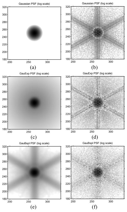
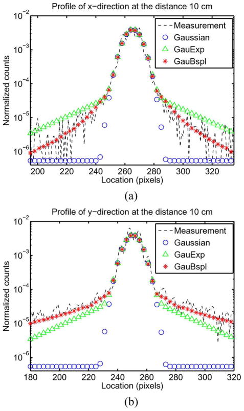
Fig. 3(a), (c), and (e) shows the fitted CDR images with the models of Gaussian, GauExp, and GauBspl. Fig. 3(b), (d), and (f) shows the absolute difference between the measured and fitted CDRs for the three different models. The Gaussian model ignored the septal penetration tails and the GauExp model tried to account for those tails by using a rotationally-invariant function. On the other hand, the GauBspl model represented the details of the septal penetration component well as seen in Fig. 3(e). The difference image between the GauBspl model and the measurement contains very little evidence of the septal penetration tail pattern as shown in Fig. 3(f). A horizontal profile (which passes through a septal penetration tail and corresponds to one azimuthal angle) and a vertical profile (which avoids passing through a tail and corresponds to a different azimuthal angle) for the normalized CDR are shown in Fig. 4. The GauExp values fall below the measured values in one case and above them in the other because GauExp averaged the values from the entire range of azimuthal angles. In contrast, GauBspl values match the measured CDR values for both profiles.
Fig. 3.
The fitted CDR, (a), (c), and (e), and the absolute difference between the fitted and measured CDR, (b), (d), and (f), for each fitting method (Gaussian, GauExp, and GauBspl) at 10 cm. The images are shown on a logarithmic grey scale. The GauBspl model describes the penetration tails of the CDR the best. (a) Gaussian. (b) |Gaussian − Measurement|. (c) GauExp. (d) |GauExp − Measurement|. (e) GauBspl. (f) |GauBspl − Measurement|.
Fig. 4.
Normalized CDR profiles for the measurement and for each fitting method (Gaussian, GauExp, and GauBspl), at 10 cm. The profile in the x direction is shown in (a) and that in the y direction in (b). GauBspl matched the measured CDR shape best in both directions. (a) x profile. (b) y profile.
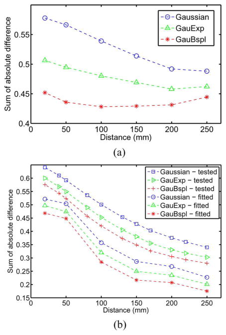
Lastly, Fig. 5 shows quantitative results by measuring the sum of the absolute difference between the measured (normalized) CDR and the fitted (normalized) CDR for the Gaussian, GauExp, and GauBspl models. Fig. 5(a) from the experimental CDR measurements shows that overall the fitting was improved by using the GauBspl model compared to using the Gaussian and GauExp models at all measured distances. Similar results were obtained from an initial set of MC simulated CDRs as shown in the bottom three plots, labeled with the extension [-fitted], of Fig. 5(b). We also compared the fitted CDR using this initial MC simulation with another set of MC simulated CDRs generated using a different random seed at 11 distances. The absolute difference between them for all three models as shown in the top three plots, labeled with the extension [-tested], of Fig. 5(b) shows that our proposed GauBspl model can represent the CDRs at various distances better than the Gaussian and GauExp models. The different random seed did change the total difference at each distance, but did not affect the ranking of the three methods.
Fig. 5.
Sum of the absolute differences between the measured and fitted PSFs versus distance for all three models: Gaussian, GauExp, and GauBspl. The three plots in (a) are using the experimentally measured CDRs. The bottom three lines in (b), labeled with the extension [-fitted], are from an initial set of MC simulated CDRs. The other three plots (top three) in (b), labeled with the extension [-tested], are from a second set of MC simulated CDRs generated using a different seed. All three comparisons show that our proposed GauBspl model can represent the CDRs at various distances better than the Gaussian and GauExp models. (a) Experimental measurements. (b) MC simulations.
We observed that our proposed GauBspl model yielded the best fit to the CDR measurement qualitatively and quantitatively. Section VI examines how this improvement in fitting the CDR affected quantification accuracy.
B. Hot Phantom Studies
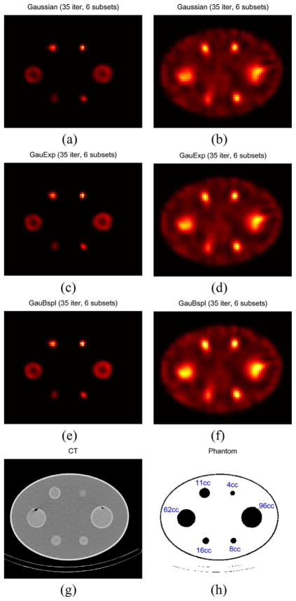
Fig. 6(a), (c), and (e) shows three reconstructed SPECT images at 35 iterations (six subsets) using the Gaussian, GauExp, and GauBspl models for the hot phantom without background activity. Fig. 6(b), (d), and (f) show similar images for the hot phantom with background activities. Fig. 6(g) and (h) shows the CT and schematic images of the phantom. It can perhaps be discerned that the GauBspl method increased the image intensity in the spheres compared to the Gaussian and GauExp methods.
Fig. 6.
Transaxial OSEM SPECT images of 3-D “hot-sphere” phantom without (no bck), (a), (c), and (e), and with background (with bck), (b), (d), and (f), activities at 35 iterations (six subsets) using three different CDR models: Gaussian, GauExp, and GauBspl. CT image (g) and schematic image (h) show the size of the spheres. The GauBspl method increased the image intensity in the spheres compared to the Gaussian and GauExp methods. Note that not all spheres are centered on the same axial plane. (a) Gaussian, no bck. (b) Gaussian, with bck. (c) GauExp, no bck. (d) GauExp, with bck. (e) GauBspl, no bck. (f) GauBspl, with bck. (g) CT. (h) Schematic image.
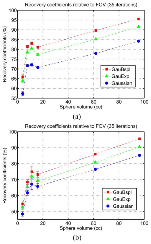
Fig. 7 shows that the GauBspl CDR compensation method yielded higher RC values than the other methods (Gaussian or GauExp) for all spheres. For the phantom without background activity, GauBspl yielded 12.9%–15.7% higher RC’s than the Gaussian method and 2.8%–5.4% higher RC’s than the GauExp method. For the phantom with background activity, it yielded 10.6%–13.0% higher RC’s than the Gaussian method and 3.7%–6.6% higher RC’s than the GauExp method. All improvements of the GauBspl method were achieved with a negligible increase of the standard deviation of the RC. Note that the RC value is “usually” larger for the larger ROIs, but the relationship to size is not linear and not monotonically increasing. This phenomenon was also observed in our XCAT phantom study of Section V-D. It may be because the RC depends not only on count “spill-out” but also on the “spill-in” effects, which depend on the activity in nearby structures, and/or because these RCs had not converged to final values due to our choice of only 35 iterations. Further investigation is necessary to explain the phenomenon.
Fig. 7.
RCs of phantom (a) without and (b) with background activity as a function of sphere volume. The GauBspl CDR model yielded higher RC values than the Gaussian or GauExp models for all spheres. (a) RC (no bck) versus sphere volume. (b) RC (with bck) versus sphere volume.
C. Patient Study
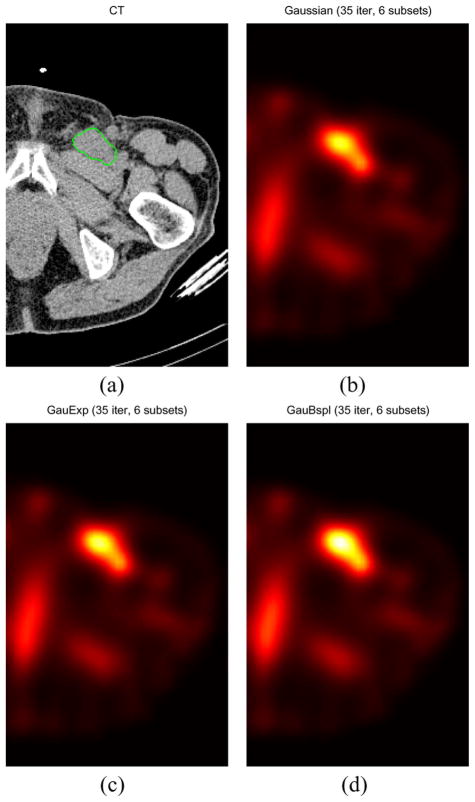
Fig. 8 shows the transaxial SPECT images using the three different CDR models and one CT image with a delineated tumor (left inguinal tumor, 38 cc). The GauBspl method yielded increased image intensity compared to the Gaussian and GauExp methods. The CR of the GauBspl method was 12.4% higher than the CR of the Gaussian method and 6.4% higher than the CR of the GauExp method. These results imply that our proposed method increased the RC compared to the Gaussian and GauExp methods, which is consistent with the results of our hot phantom studies. However, in this patient study, we do not know whether our proposed method resulted in improvement of absolute activity quantification since we do not know the amount of true activities.
Fig. 8.
(a) CT image with delineated tumor and (b)–(d) SPECT images with different CDR models of a patient. The GauBspl method yielded increased image intensity and CR’s (implicitly RC’s) compared to the Gaussian and GauExp methods. (a) CT image. (b) SPECT image (Gaussian). (c) SPECT image (GauExp). (d) SPECT image (GauBspl).
D. XCAT Phantom Study With MC Simulation
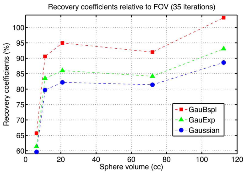
Fig. 9 shows the true and reconstructed SPECT images using three different CDR models with the XCAT phantom. The GauBspl method produced somewhat increased image intensity compared to the other Gaussian and GauExp methods. Fig. 10 shows the quantification results of the XCAT phantom study. The GauBspl approach yielded 10.2%–16.5% higher RC’s than the Gaussian method and 7.0%–10.8% higher RC’s than the GauExp method for the different-size spherical tumors.
Fig. 9.
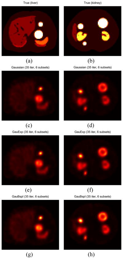
Transaxial true images of the XCAT phantom with five tumors near the liver (a) and the kidney (b). SPECT images were reconstructed using the three different CDR models for the liver (c), (e), and (g), and for the kidney (d), (f), and (h). The GauBspl method produced somewhat increased image intensity compared to the Gaussian and GauExp methods. (a) XCAT phantom (liver). (b) XCAT phantom (kidney). (c) Gaussian (liver). (d) Gaussian (kidney). (e) GauExp (liver). (f) GauExp (kidney). (g) GauBspl (liver). (h) GauBspl (kidney).
Fig. 10.
Recovery coefficients from the XCAT phantom plotted as a function of sphere volume. The GauBspl approach yielded higher RC’s than the Gaussian and GauExp methods for all spherical tumors.
VI. Discussion
We evaluated our method and showed quantification improvement in I-131 SPECT imaging for oncologic applications (tumor dosimetry). However, our proposed method can potentially be useful in improving SPECT quantitative accuracy using any radionuclides that emit medium or high-energy photons for various applications with other organs.
We measured an I-131 point source that had a 7 mm diameter because of the difficulties in constructing a smaller point source with significant activity. We studied the effect of potentially reducing the size of the point source using MC simulation. We simulated a 7 mm diameter and a 1 mm diameter point source and measured the full-width half-maximum (FWHM) of the Gaussian fit for both. The MC results show that, at 2, 10, and 15 cm, the FWHM of the 7 mm point source was 8.5, 15.1, and 18.6 mm, respectively, while the FWHM of the 1 mm point source was 7.4, 14.8, and 18.2 mm, respectively. In our XCAT phantom study, using the results from the smaller point source resulted in a RC difference (| RC using 7 mm point source − RC using 1 mm point source|/RC using 1 mm point source ×100) that ranged from 0.6%–2.3%. The RC differences, therefore, seem relatively small. However, recently, small beads with Tc-99m (180–500 μm size) were used as point sources in micro SPECT-CT studies [30]. The same beads could potentially be used with I-131 to improve the accuracy of our present CDR measurements.
The location of the point source relative to the septa can also change the quantification result since the sensitivity depends on the location. We ran another MC simulation with the point source at two locations (center of the image plane and 2 mm shifted from the center in both the x and the y direction). An observed increase of the FWHM became smaller as the distance from object to camera became larger. The FWHM changed from 8.5 to 10.9 mm at 2 cm, from 11.2 to 12.1 mm at 5 cm, and from 15.0 to 15.1 mm at 15 cm. In our XCAT phantom study, these differences resulted in a 0.5%–3.1% difference in the RC value (|RC using centered point source - RC using shifted point source| /RC using centered point source × 100). One may reduce this variability by measuring the point source at more than one location for close distances (e.g., 2 cm) and averaging the results. Compensating for the sensitivity difference at different locations would require computationally demanding MC simulations in the forward projection.
Our proposed function fitting based approach is an alternative way to model the CDR compared to MC-based CDR modeling [2], [3], [14]. The MC-based CDR modeling method requires accurate SPECT simulations for a given scanner, but our proposed B-spline PSF template approach requires only the measured CDRs from the scanner. However, this work did not assess the relative merits of the two methods. In a future study, it would be interesting to compare the performance difference between the function fitting based and the MC-based CDR models.
We used unregularized OSEM (35 iterations and six subsets), which is the reconstruction method used in our I-131 SPECT-CT imaging-based dosimetry studies [27]. In our phantom studies, we observed that more iterations yielded higher RC values, but they also yielded noisier images due to the ill-posed nature of the unregularized optimization. The unregularized optimization also usually yielded lesions or spheres with edge artifacts [1] [higher activities around the sharp edges—see Fig. 6(a)–(e)]. Edge-preserving regularization methods may be able to reduce both the edge artifacts and the noise [31].
VII. Conclusion
We developed a B-spline PSF template approach to CDR modeling for more accurate quantification in SPECT. It is most appropriate for radionuclides that emit medium or high-energy photons, such as I-131. Our proposed method yielded CDRs that better matched the measured CDRs compared to previous function fitting methods using Gaussian or Gaussian plus exponential functions. We also showed that this improved CDR fitting translated into substantially improved SPECT quantification, as determined by increased RCs, in experimental and digital phantom studies.
Acknowledgments
This work was supported by the National Institutes of Health (NIH) under Grant 2RO1 EB001994.
The authors would like to thank the anonymous reviewers and Dr. K. F. Koral for helpful comments that improved this paper.
Footnotes
Color versions of one or more of the figures in this paper are available online at http://ieeexplore.ieee.org.
Contributor Information
Se Young Chun, Email: delight@umich.edu, Department of Electrical Engineering and Computer Science and Radiology, University of Michigan, Ann Arbor, MI 48109 USA.
Jeffrey A. Fessler, Email: fessler@umich.edu, Department of Electrical Engineering and Computer Science, University of Michigan, Ann Arbor, MI 48109 USA.
Yuni K. Dewaraja, Email: yuni@umich.edu, Department of Radiology, University of Michigan, Ann Arbor, MI 48109 USA.
References
- 1.Tsui BMW, Frey EC, Zhao X, Lalush DS, Johnston RE, McCartney WH. The importance and implementation of accurate 3d compensation methods for quantitative SPECT. Phys Med Biol. 1994;39(3):509–530. doi: 10.1088/0031-9155/39/3/015. [DOI] [PubMed] [Google Scholar]
- 2.Ljungberg M, Sjogreen K, Liu X, Frey E, Dewaraja Y, Strand SE. A 3-dimensional absorbed dose calculation method based on quantitative SPECT for radionuclide therapy: Evaluation for 131I using Monte Carlo simulation. J Nucl Med. 2002;43(8):1101–1109. [PMC free article] [PubMed] [Google Scholar]
- 3.He B, Du Y, Song X, Segars WP, Frey EC. A Monte Carlo and physical phantom evaluation of quantitative in-111 SPECT. Phys Med Biol. 2005 Sep;50(17):4169–4186. doi: 10.1088/0031-9155/50/17/018. [DOI] [PubMed] [Google Scholar]
- 4.Dewaraja YK, Wilderman SJ, Ljungberg M, Koral KF, Zasadny K, Kaminiski MS. Accurate dosimetry in 131I radionuclide therapy using patient-specific, 3-dimensional methods for SPECT reconstruction and absorbed dose calculation. J Nucl Med. 2005;46(5):840–849. [PMC free article] [PubMed] [Google Scholar]
- 5.Larsson A, Ljungberg M, Mo SJ, Riklund K, Johansson L. Correction for scatter and septal penetration using convolution subtraction methods and model-based compensation in 123 i brain SPECT imaging—A Monte Carlo study. Phys Med Biol. 2006;51(22):5753–5767. doi: 10.1088/0031-9155/51/22/003. [DOI] [PubMed] [Google Scholar]
- 6.Moody J, Dewaraja YK, Ficaro EP. Resolution and noise properties of 123I-MIBG SPECT with collimator-detector response modeling. IEEE Nucl Sci Symp Conf Rec. 2011 Oct;:2779–2786. [Google Scholar]
- 7.Dewaraja YK, Ljungberg M, Koral KF. Characterization of scatter and penetration using Monte Carlo simulation in 131I imaging. J Nucl Med. 2000 Jan;41(1):123–130. [PMC free article] [PubMed] [Google Scholar]
- 8.Du Y, Tsui BMW, Frey EC. Model-based compensation for quantitative 123 I brain SPECT imaging. Phys Med Biol. 2006;51(5):1269–1269. doi: 10.1088/0031-9155/51/5/016. [DOI] [PubMed] [Google Scholar]
- 9.Cot A, Jane E, Sempau J, Falcon C, Bullich S, Pavia J, Calvino F, Ros D. Modeling of high-energy contamination in SPECT imaging using Monte Carlo simulation. IEEE Trans Nucl Sci. 2006 Feb;53(1):198–203. [Google Scholar]
- 10.Moore SC, Ouyang J, Park MA, Fakhri GE. Monte Carlo-based compensation for patient scatter, detector scatter, and crosstalk contamination in In-111 SPECT imaging. Nucl Instrum Methods Phys Res Sect A: Accel, Spect, Detectors Assoc Equip. 2006;569(2):472–476. [Google Scholar]
- 11.Staelens S, de Wit T, Beekman F. Fast hybrid SPECT simulation including efficient septal penetration modelling (SP-PSF) Phys Med Biol. 2007;52(11):3027–3043. doi: 10.1088/0031-9155/52/11/007. [DOI] [PubMed] [Google Scholar]
- 12.Metz CE, Atkins FB, Beck RN. The geometric transfer function component for scintillation camera collimators with straight parallel holes. Phys Med Biol. 1980 Nov;25(6):242–250. doi: 10.1088/0031-9155/25/6/003. [DOI] [PubMed] [Google Scholar]
- 13.Frey EC, Tsui BMW. Collimator-detector response compensation in SPECT. In: Zaidi H, editor. Quantitative Analysis in Nuclear Medicine Imaging. New York: Springer; 2006. pp. 141–166. [Google Scholar]
- 14.Liu S, Farncombe TH. Collimator-detector response compensation in quantitative SPECT reconstruction. IEEE Nucl Sci Symp Conf Rec. 2007 Nov;5:3955–3960. [Google Scholar]
- 15.Song X, Segars WP, Du Y, Tsui BMW, Frey EC. Fast modelling of the collimator-detector response in Monte Carlo simulation of SPECT imaging using the angular response function. Phys Med Biol. 2005;50(8):1791–1804. doi: 10.1088/0031-9155/50/8/011. [DOI] [PubMed] [Google Scholar]
- 16.Assie K, Gardin I, Vera P, Buvat I. Validation of the Monte Carlo simulator GATE for Indium-111 imaging. Phys Med Biol. 2005;50:3113–3125. doi: 10.1088/0031-9155/50/13/010. [DOI] [PubMed] [Google Scholar]
- 17.Rault E, Staelens S, Holen RV, Beenhouwer JD, Vandenberghe S. Fast simulation of yttrium-90 bremsstrahlung photons with GATE. Med Phys. 2010;37(6):2943–2950. doi: 10.1118/1.3431998. [DOI] [PubMed] [Google Scholar]
- 18.Koral KF, Yendiki A, Lin Q, Dewaraja YK, Fessler JA. Determining total I-131 activity within a VoI using SPECT, a UHE collimator, OSEM, and a constant conversion factor. IEEE Trans Nucl Sci. 2004 Jun;51(3):611–618. [Google Scholar]
- 19.Furenlid L, Wilson D, Chen YC, Kim H, Pietraski P, Crawford M, Barrett H. FastSPECT II: A second-generation high-resolution dynamic SPECT imager. IEEE Trans Nucl Sci. 2004 Jun;51(3):631–635. doi: 10.1109/TNS.2004.830975. [DOI] [PMC free article] [PubMed] [Google Scholar]
- 20.van der Have F, Vastenhouw B, Ramakers RM, Branderhorst W, Krah JO, Ji C, Staelens SG, Beekman FJ. U-SPECT-II: An ultra-high-resolution device for molecular small-animal imaging. J Nucl Med. 2009 Apr;50(4):599–605. doi: 10.2967/jnumed.108.056606. [DOI] [PubMed] [Google Scholar]
- 21.Dewaraja YK, Ljungberg M, Fessler JA. 3-D Monte Carlo-based scatter compensation in quantitative I-131 SPECT reconstruction. IEEE Trans Nucl Sci. 2006 Feb;53(1):181–188. doi: 10.1109/TNS.2005.862956. [DOI] [PMC free article] [PubMed] [Google Scholar]
- 22.Coleman TF, Li Y. An interior, trust region approach for nonlinear minimization subject to bounds. SIAM J Optim. 1996;6(2):418–445. [Google Scholar]
- 23.Unser M, Aldroubi A, Eden M. B-spline signal processing: Part I—Theory. IEEE Trans Signal Process. 1993 Feb;41(2):821–833. [Google Scholar]
- 24.Liu D, Nocedal J. On the limited memory method for large scale optimization. Math Programm B. 1989;45(3):503–528. [Google Scholar]
- 25.Ljungberg M, Strand SE. A Monte Carlo program for the simulation of scintillation camera characteristics. Comput Methods Programs Biomed. 1989;29(4):257–272. doi: 10.1016/0169-2607(89)90111-9. [DOI] [PubMed] [Google Scholar]
- 26.Zeng GL, Gullberg GT. Frequency domain implementation of the three-dimensional geometric point response correction in SPECT imaging. IEEE Trans Nucl Sci. 1992 Oct;39(5):1444–1453. [Google Scholar]
- 27.Dewaraja YK, Schipper MJ, Roberson PL, Wilderman SJ, Amro H, Regan DD, Koral KF, Kaminski MS, Avram AM. 131I-tositumomab radioimmunotherapy: Initial tumor dose-response results using 3-dimensional dosimetry including radiobiologic modeling. J Nucl Med. 2010;51(7):1155–1162. doi: 10.2967/jnumed.110.075176. [DOI] [PMC free article] [PubMed] [Google Scholar]
- 28.Segars WP, Mahesh M, Beck TJ, Frey EC, Tsui BMW. Realistic CT simulation using the 4D XCAT phantom. Med Phys. 2008 Aug;35(8):3800–3808. doi: 10.1118/1.2955743. [DOI] [PMC free article] [PubMed] [Google Scholar]
- 29.Fessler JA, Rogers WL. Spatial resolution properties of penalized-likelihood image reconstruction methods: Space-invariant tomographs. IEEE Trans Imag Process. 1996 Sep;5(9):1346–1358. doi: 10.1109/83.535846. [DOI] [PubMed] [Google Scholar]
- 30.Ji C, van der Have F, van Andela HG, Ramakers R, Beekman F. Accurate coregistration between ultra-high-resolution micro-SPECT and circular cone-beam micro-CT scanners. Int J Biomed Imag. 2010;2010(2010):12–12. doi: 10.1155/2010/654506. [DOI] [PMC free article] [PubMed] [Google Scholar]
- 31.Dewaraja YK, Koral KF, Fessler JA. Regularized reconstruction in quantitative SPECT using CT side information from hybrid imaging. Phys Med Biol. 2010 May;55(9):2523–2529. doi: 10.1088/0031-9155/55/9/007. [DOI] [PMC free article] [PubMed] [Google Scholar]


