Proterozoic ocean redox and biogeochemical stasis

Abstract

The partial pressure of oxygen in Earth’s atmosphere has increased dramatically through time, and this increase is thought to have occurred in two rapid steps at both ends of the Proterozoic Eon (∼2.5–0.543 Ga). However, the trajectory and mechanisms of Earth’s oxygenation are still poorly constrained, and little is known regarding attendant changes in ocean ventilation and seafloor redox. We have a particularly poor understanding of ocean chemistry during the mid-Proterozoic (∼1.8–0.8 Ga). Given the coupling between redox-sensitive trace element cycles and planktonic productivity, various models for mid-Proterozoic ocean chemistry imply different effects on the biogeochemical cycling of major and trace nutrients, with potential ecological constraints on emerging eukaryotic life. Here, we exploit the differing redox behavior of molybdenum and chromium to provide constraints on seafloor redox evolution by coupling a large database of sedimentary metal enrichments to a mass balance model that includes spatially variant metal burial rates. We find that the metal enrichment record implies a Proterozoic deep ocean characterized by pervasive anoxia relative to the Phanerozoic (at least ∼30–40% of modern seafloor area) but a relatively small extent of euxinic (anoxic and sulfidic) seafloor (less than ∼1–10% of modern seafloor area). Our model suggests that the oceanic Mo reservoir is extremely sensitive to perturbations in the extent of sulfidic seafloor and that the record of Mo and chromium enrichments through time is consistent with the possibility of a Mo–N colimited marine biosphere during many periods of Earth’s history.

The chemical composition of the oceans has changed dramatically with the oxidation of Earth’s surface (1), and this process has profoundly influenced and been influenced by the evolutionary and ecological history of life (2). The early Earth was characterized by a reducing ocean-atmosphere system, whereas the Phanerozoic Eon (< 0.543 Ga) is known for a stably oxygenated biosphere conducive to the radiation of large, metabolically demanding animal body plans and the development of complex ecosystems (3). Although a rise in atmospheric O₂ is constrained to have occurred near the Archean–Proterozoic boundary (∼2.4 Ga), the redox characteristics of surface environments during Earth’s middle age (1.8–0.543 Ga) are less well known. The ocean was historically envisaged to have become ventilated at ∼1.8 Ga based on the disappearance of economic iron deposits (banded iron formations; 2), but over the past decade it has been commonly assumed that the mid-Proterozoic Earth was home to a globally euxinic ocean, a model derived from theory (4) and supported by evidence for at least local sulfidic conditions in Proterozoic marine systems (5–8). However, the record of sedimentary molybdenum (Mo) enrichment through Earth’s history has been interpreted to suggest that euxinia on a global scale was unlikely (9).

More recently, it has been proposed that the deep ocean remained anoxic until the close of the Proterozoic, but that euxinia was limited to marginal settings with high organic matter loading (10–13). In anoxic settings with low dissolved sulfide levels, ferrous iron will accumulate—thus these anoxic but nonsulfidic settings have been termed “ferruginous” (10). This model has also found support in at least local evidence for ferruginous marine conditions during the mid-Proterozoic (12, 13). However, it has been notoriously difficult to estimate the extent of this redox state on a global scale, even in the much more recent ocean—largely because most of the ancient deep seafloor has been subducted.

In principle, trace metal enrichments in anoxic shales can record information about seafloor redox on a global scale. Following the establishment of pervasive oxidative weathering after the initial rise of atmospheric oxygen at ∼2.4 Ga (14), the concentration of many redox-sensitive elements in the ocean has been primarily controlled by marine redox conditions. For example, in today’s well-oxygenated oceans, Mo is the most abundant transition metal in seawater (∼107 nM; ref. 15), despite its very low crustal abundance (∼1–2 ppm; ref. 16). Under sulfidic marine conditions the burial fluxes of Mo exceed those in oxygenated settings by several orders of magnitude (17). Hence, it follows that when sulfidic conditions are more widespread than today, global seawater concentrations of Mo will be much lower. Because the enrichment of Mo in sulfidic shales scales with dissolved seawater Mo concentrations (18), Mo enrichments in marine shales (independently elucidated as being deposited under euxinic conditions with a strong connection to the open ocean) can be used to track the global extent of sulfidic conditions (9). Substantial Mo enrichment in an ancient euxinic marine shale, such as occurs in modern euxinic marine sediments, implies that sulfidic bottom waters represent a very small extent of the global seafloor.

In principle, a similar approach can be used with other metals such as Cr, which, importantly, will also be reduced and buried in sediments under anoxic conditions but without the requirement of free sulfide. Chromium is readily immobilized as (Fe,Cr)(OH)₃ under ferruginous conditions (19, 20) and will be reduced and rendered insoluble by reaction with a wide range of other reductants under sulfidic or even denitrifying conditions (21–23). Thus, comparing Mo enrichments in independently constrained euxinic shales and Cr enrichments in independently constrained anoxic shales can offer a unique and complementary perspective on the global redox landscape of the ocean.

A better understanding of the marine Mo cycle in Proterozoic oceans may also illuminate key controlling factors in biological evolution and ecosystem development during the emergence of eukaryotic life. The biogeochemical cycles of marine trace elements form a crucial link between the inorganic chemistry of seawater and the biological modulation of atmospheric composition. The availability of iron, for example, has been invoked as a primary control on local carbon export fluxes and atmospheric pCO₂ on glacial–interglacial timescales (24, 25). However, the leverage exerted by Fe on recent oceanic carbon fixation is most fundamentally driven by the sparing solubility of Fe in an ocean that is well-ventilated by an oxygen-rich atmosphere. By analogy, on a more reducing Earth surface Mo is likely to be a key colimiting trace nutrient given its importance in biological nitrogen fixation, assimilatory/dissimilatory nitrate reduction, and a number of other metabolically significant electron transfer processes (26–28).

To move forward in our understanding of Proterozoic redox evolution, we present a unique view of Cr and Mo enrichments in anoxic shales and a complementary modeling approach to interpret these data. From this vantage point, we present evidence that anoxic conditions were a globally important feature in the mid-Proterozoic ocean. In our analysis, we take anoxic environments to include those that are euxinic (anoxic and H₂S-rich), ferruginous (anoxic and Fe²⁺-rich), and NO₃⁻-buffered (i.e., anoxic but with low concentrations of both H₂S and Fe²⁺). We note, however, that the latter environments are likely to be spatially and temporally limited given the relatively low concentration (and thus redox buffering capacity) of NO₃⁻ in seawater, particularly during the Proterozoic (29).

Despite evidence for pervasive marine anoxia during the Proterozoic, we highlight that euxinia covered only a small portion of the seafloor. On this basis, we present a framework for linking Mo enrichments to seawater Mo concentrations that points toward Mo–N colimitation in the Proterozoic ocean. Therefore, despite a more limited extent of euxinia than previously envisaged, life in the Proterozoic ocean was heavily influenced by a prevalence of sulfide in the water column that far exceeded the small amounts of euxinia that characterize the modern ocean.

Mid-Proterozoic Geochemical Record

We present a record of Cr and Mo enrichments in anoxic and euxinic black shales through time (Fig. 1). Samples for this study (n > 3,000) come from our analytical efforts and a literature survey (Fig. S1 and Table S1). Our own data include results from over 300 Precambrian samples and modern anoxic systems. Samples were filtered for basic lithology (fine-grained siliciclastics) using a combination of basic sedimentary petrology and major-element thresholds. We relied on well-established paleoproxies rooted in Fe–S systematics to infer the redox state of the water column overlying the site of shale deposition. Importantly, these paleoredox proxies are calibrated to delineate anoxic settings (where Cr will be reduced and buried) and euxinic settings (where both Cr and Mo will be reduced/sulfidized and buried). The Fe–S paleoproxies have recently been reviewed in detail (30, 31), and full information on sample filters is provided in SI Discussion. We emphasize the noncircularity of our approach to analyzing the shale record—specifically, we constrained local paleoredox to have been anoxic or euxinic with no appeal to sedimentary trace metal enrichments as fingerprints of those conditions. This approach allows us to use the metal enrichments themselves as proxies for broader ocean redox state and its control on the ocean-wide inventories of those metals.

Fig. 1.

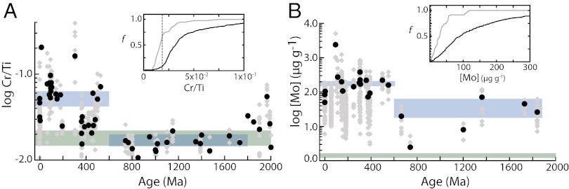
Sedimentary Cr (A) and Mo (B) enrichments in anoxic and euxinic black shales through time. Because of the relatively high Cr content of typical detrital material, Cr enrichments are expressed as Cr/Ti ratios. Gray diamonds represent all filtered data, whereas black circles represent temporally binned averages. Blue boxes show the total mean (±95% confidence interval) of temporally binned averages for the mid-Proterozoic and Phanerozoic (SI Discussion). (Insets) Cumulative frequency distribution of enrichments for the mid-Proterozoic (gray curve) and the Phanerozoic (black curve). Green boxes show the composition of average post-Archean upper crust (31–33) used to approximate the detrital input. Note the log scale.

There are significant Mo enrichments in mid-Proterozoic (∼1.8–0.6 Ga) euxinic shales (Fig. 1B). However, these enrichments are significantly lower than those observed in late Proterozoic and Phanerozoic euxinic equivalents (9). Proterozoic enrichments range from less than 10 to greater than 100 ppm, compared with concentrations on the order of ∼1–2 ppm in average upper crust (16). The total mean for temporally binned mid-Proterozoic euxinic shale data (2.0–0.74 Gya) is 40.5 ppm (±22.5 at the 95% confidence level) compared with the Phanerozoic where the total mean is 170.2 ppm (±33.4 ppm at the 95% confidence level).

In strong contrast with the Mo record, there are no discernible Cr enrichments in mid-Proterozoic anoxic shales. We report Cr enrichments by normalizing to Ti content, as detrital inputs of Cr to marine sediments can be substantial and are greatly in excess of those for Mo. The total mean for Cr/Ti values for mid-Proterozoic anoxic shales is 1.69 × 10⁻² (ppm/ppm), and the 95% confidence interval (1.45 × 10⁻² to 1.93 × 10⁻²) is indistinguishable from post-Archean average upper crust (32–34) (Fig. 1A). There is a marked increase in Cr/Ti ratios after the late Proterozoic, with Phanerozoic shales showing Cr/Ti values indicating enrichments of tens to hundreds of ppm. This pattern is mirrored in the sharp rise in Mo enrichments through the same interval.

We hypothesize that the enrichment trends for both metals reflect the progressive expansion of marine anoxia between 2.0 and 1.8 Ga and persistent oceanic Cr drawdown during the mid-Proterozoic. Because of the different conditions required for the reduction, immobilization, and accumulation in sediments for Cr (anoxic) and Mo (euxinic), we suggest that a relatively small proportion of oceanic anoxia was represented by euxinic conditions, which allowed a moderate although muted seawater Mo reservoir to coexist with a strongly depleted Cr reservoir. We note also that the much greater density of Cr data once the datasets have been filtered for local redox suggests qualitatively that anoxic shales were much more common than euxinic shales during the Proterozoic.

In contrast, the Phanerozoic record is generally characterized by elevated enrichments of both elements, suggesting that for most of the Phanerozoic both anoxic and euxinic conditions were less spatially and/or temporally widespread. Comparatively short-lived Phanerozoic oceanic anoxic events (OAEs), such as those famously expressed in the Mesozoic, are a notable exception. We suggest that combining enrichment records for elements that respond to the presence of free HS⁻ in anoxic marine environments (Mo, Zn, etc.) with elements that respond to anoxia more generally (Cr, Re, V, etc.) may allow us to place more detailed constraints on the fabric of seafloor redox and bioinorganic feedbacks throughout Earth’s history. We can then expand this approach by interpreting such data within a global mass balance framework.

Interpreting the Enrichment Record: Model for Global Mass Balance and Burial in Marine Sediments

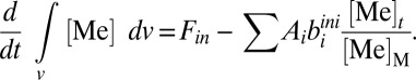
Our quantitative model begins with a conventional mass balance formulation (35), in which the ocean is treated as a single well-mixed reservoir (Fig. S2)—a reasonable assumption given the relatively long residence times of the elements of interest (SI Discussion). The globally averaged concentration of a metal in the ocean evolves as

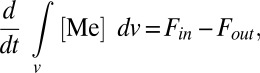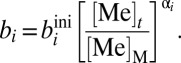
where [Me] represents the seawater concentration of a given metal, integrated over ocean volume v. The terms F_in and F_out represent input and output fluxes, respectively. In both cases, input fluxes associated with riverine delivery and/or seawater–basalt interaction are grouped into a single input term (F_in; SI Discussion and Fig. S3), whereas output fluxes (F_out) are broken into burial terms specific to each metal cycle (Fig. S2 and Tables S2–S6). Riverine input dominates the overall input flux for both metals (SI Discussion), and this flux is unlikely to have varied significantly (relative to variations in the removal fluxes) after Earth’s initial oxygenation. Sink fluxes (burial in sediments) are a function of the characteristic burial rate and areal extent of a given sink environment (i):

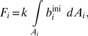where A_i represents the seafloor area of each sink environment (oxic, ferruginous, sulfidic, etc.), and b_iⁱⁿⁱ represents the globally averaged initial burial rate characteristic of that environment. In this equation, k is a reaction coefficient that relates the burial flux to the seawater concentration. For a strictly first-order model, k = [Me]_t/[Me]_M, where [Me]_t is the mean oceanic concentration of a given metal at time t, and [Me]_M is the modern seawater concentration. As previously noted (36), this kind of first-order mass balance approach to specifying removal fluxes is a specific variant of the more generalized case:

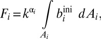where α = 1.0.

Combining the above terms yields an expression for each removal flux:

Following previous approaches, we first assume that α = 1.0 (i.e., first-order mass balance). This approach is grounded in the notion that the burial rate of a metal in a given sink environment will scale in a roughly linear fashion with the ambient seawater reservoir size (18, 35). After substitution and rearrangement of the above equations, we arrive at a generalized mass balance equation for both metals:

Because we are mainly interested in broad (∼10⁶ y) shifts in deep ocean redox, we assume steady-state conditions for both metal systems. Assuming steady state (i.e., d[Me]/dt = 0) yields an expression for the average oceanic concentration of a given metal:

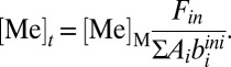An important component of our model is the specification of spatially variant metal burial rates. Most past treatments of oceanic metal mass balance suffer from the physically unrealistic assumption that the metal burial rates characteristic of modern environments, typically encountered in restricted or marginal settings such as the Black Sea and Cariaco Basin, where overall sediment and carbon fluxes are high, can be scaled to very large regions of the abyssal seafloor where bulk sediment delivery and organic carbon fluxes are typically much lower (37, 38). We have attempted to avoid the same oversimplification by coupling an algorithm that addresses carbon flux to the seafloor as a function of depth (39) to a polynomial function fitted to bathymetric data (40) and by tuning an imposed burial ratio parameter (R_Me/C) to reproduce the modern globally averaged burial rate for each metal (SI Discussion and Fig. S4).

The essential assumption here is that a given region of the seafloor will have a characteristic “burial capacity” for Mo and Cr, regulated to first order by carbon flux to the sediment, and that this capacity will only be realized if the environment is anoxic (in the case of Cr) or euxinic (in the case of Mo). From a mechanistic perspective, this approach builds from clear evidence that the burial in sediments of many redox sensitive metals in anoxic settings scales strongly with carbon flux to the sediments (18, 41, 42). We hold that this approach allows for a more realistic depiction of perturbations to seawater metal inventories as a function of seafloor redox dynamics by smoothly decreasing globally averaged burial rates as larger regions of the seafloor become anoxic (Cr) or sulfidic (Mo).

Interpreting the Enrichment Record: Model Results

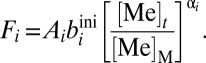
Our approach assumes, by definition, that the burial rate of a given metal in an authigenically active environment (i.e., environments that remove Cr and/or Mo from seawater and sequester them within the sediment column) scales with the ambient concentration in seawater:

The seawater reservoir is controlled largely by how this relationship is expressed on a global scale, but this relationship will also apply to individual settings or regions of the seafloor. As a result, we can envision a generalized authigenically active setting and estimate sedimentary metal enrichments as a function of seawater concentration, in turn controlled by the relative areas of different redox environments on a global scale.

The results of such an exercise are shown in Fig. 2. Here, we have used as our starting point burial rates and overall sediment mass accumulation rates from one of the best-characterized perennially euxinic basins on the modern Earth, the Cariaco Basin in Venezuela. Our purpose here is to depict a generalized setting accumulating Cr and Mo within sediments that has a relatively open connection to the seawater metal reservoir(s), and for that reason we have chosen the Cariaco Basin over the highly restricted Black Sea, which shows clear local reservoir effects for Mo (18). In essence, we pose the question, “How would an anoxic or euxinic continental margin or epicontinental environment, such as that represented in the marine black shale record, respond to a particular perturbation to seafloor redox state?” We can then scale this relationship to spatially varying organic carbon burial and bulk sedimentation to inform metal uptake away from the continental margin.

Fig. 2.

Estimated authigenic sedimentary enrichments ([X]_auth) for Cr (A) and Mo (B) in a generalized anoxic or euxinic setting, respectively, as a function of anoxic and sulfidic seafloor area (A_anox, A_sulf). Black curves represent a bulk mass accumulation rate of 1.0 × 10⁻² g⋅cm⁻²⋅y⁻¹, whereas gray dotted curves represent a factor of 1.5 above and below this value (SI Discussion; Fig. S5). The blue box in A represents the approximate area of seafloor anoxia required to drop below an enrichment threshold of 5 µg⋅g⁻¹, a conservative value for our purposes given the negligible enrichments recorded by mid-Proterozoic anoxic shales. The red box in B shows the approximate sulfidic seafloor area consistent with the range of mid-Proterozoic Mo enrichments, and is scaled relative to the y axis according to the 95% confidence interval of temporally binned averages shown in Fig. 1. Seafloor areas are shown as a percentage relative to modern seafloor area (%) and in terms of raw area (km²).

A striking pattern emerges when we consider the magnitude of enrichment that can be achieved in an authigenically active environment under different oceanic redox conditions (Fig. 2). If our model is correct, the negligible sedimentary Cr enrichments characteristic of the entire mid-Proterozoic would require extremely pervasive anoxic conditions. Our approach (which is likely conservative; SI Discussion) suggests that at least ∼30–40% of the seafloor must have underlain anoxic deep waters to drive Cr enrichments to crustal values for sustained periods. We stress that this is a minimum estimate, and that our results are also fully consistent with virtually complete seafloor anoxia.

The Mo enrichment record, however, tells a very different story. Enrichments in euxinic environments during the mid-Proterozoic are muted relative to the Phanerozoic, a pattern that emerges as a consequence of more widespread sulfidic deposition relative to most of the Phanerozoic and is reinforced when Mo enrichments are normalized to total organic carbon (TOC; ref. 9). However, Mo enrichments in Proterozoic euxinic environments that are mostly well above crustal values are inconsistent with pervasive, ocean-scale euxinia (Fig. 2B). Instead, our model results point to roughly ∼1–10% of the seafloor as having been euxinic during the mid-Proterozoic, although there is likely to have been dynamic expansion/contraction of the area of euxinic seafloor area within and occasionally beyond this range—as related, for example, to spatiotemporal patterns of primary production along ocean margins. A similar range of euxinic seafloor is implied for some brief periods of the Phanerozoic (43, 44), but the record of appreciable Cr enrichment during this latter phase of Earth history indicates much more spatially and temporally restricted anoxia overall.

Marine Euxinia: Global Effects of Regional Ocean Chemistry

The record of Cr and Mo enrichment, when interpreted in light of our model results, necessitates that euxinia covered a relatively small fraction of overall seafloor area during the mid-Proterozoic despite pervasive anoxic conditions on a global scale. Such a result adds to growing evidence that Proterozoic deep ocean chemistry was dominated by anoxic but nonsulfidic (ferruginous) conditions (10, 12, 13), in contrast with most modern anoxic marine settings that tend toward euxinia. Nevertheless, euxinia in the mid-Proterozoic ocean was likely orders of magnitude more widespread than today’s estimate of ∼0.1% of the seafloor, and the deleterious impacts on nutrient availability could have been enough to significantly alter global biogeochemical processes. In effect, the sensitivity of the oceanic Mo reservoir to small perturbations in the extent of sulfidic seafloor suggests that a strong distinction should be made between a sulfidic ocean in an oceanographic sense, in which a large proportion of oceanic volume and basin- or global-scale areas of the seafloor (much more than our estimate of ∼1–10%) are characterized by sulfidic waters, and an ocean that is sulfidic from a nutrient or biological perspective. From a biological perspective, trace nutrient colimitation of marine primary producers will be strongly controlled by the extent of euxinic conditions despite euxinia not being persistent throughout most of the ocean. These conditions are, of course, not mutually exclusive––a globally sulfidic ocean will almost certainly result in trace element colimitation. However, the distinction is important as it highlights the leverage that relatively small regions of the ocean can exert on the biogeochemical cycling of certain biolimiting trace elements (9, 26).

To further explore this concept, we use the model to estimate globally averaged seawater [Mo] under variable scaling between the ambient seawater concentration and burial rate within sediments. The most common approach, as discussed above, is to assume strictly first-order (i.e., linear) scaling (α = 1.0). Although data are somewhat limited and it is difficult to establish precisely what the form of this relationship should be, data from the most well-characterized perennially euxinic settings on the modern Earth suggest that this relationship may in fact be nonlinear (Fig. 3A). The effect of this parameter on steady-state globally averaged seawater [Mo] is shown in Fig. 3B. Because lowering the value for α allows for a higher burial rate (and thus removal flux from the ocean) at a given value for seawater [Mo], the concentration is ultimately drawn down to much lower steady-state values for a given perturbation.

Fig. 3.

Effects of deviating from a strictly first-order model. (A) Mo burial rates as a function of ambient dissolved Mo concentration (shown as a proportion of modern seawater [Mo]/[Mo]_M) for a range of α-values between 1.0 (strict first-order) and 0.25. Curves are calculated assuming a modern globally averaged euxinic burial rate of 1.53 µg⋅cm⁻²⋅y⁻¹. Black circles represent values for well-characterized perennially euxinic marine basins on the modern Earth [Black Sea (BS), Framvaren Fjord (FF), and the Cariaco Trench (CT)]. (B) Steady-state globally averaged seawater Mo concentrations as a function of sulfidic seafloor area (A_sulf) for different values of α. The shaded box depicts values below 10 nM.

Although the term α regulates the scaling between ambient [Mo] and Mo burial rate on a global scale in an integrated sense across diverse redox settings, it will also do so within individual authigenically active environments. Importantly, this means that the sedimentary enrichments predicted by the model for a given extent of euxinic seafloor do not vary as a function of α. Changes in this parameter are reflected by the steady-state concentration of Mo in seawater (the same applies for Cr). It is clear from this exercise (Fig. 3) that even relatively small areas of the seafloor overlain by euxinic water masses (a fraction of modern continental shelf area) are sufficient to draw the ocean’s average Mo concentration to ∼10 nM (an order of magnitude below that seen in the modern ocean), even with strictly linear scaling between ambient [Mo] and burial flux.

Further work is needed to better pinpoint the levels of seawater Mo that should be considered biologically limiting, but available evidence is consistent with biolimiting concentrations in mid-Proterozoic oceans. Culturing experiments with modern strains of diazotrophic (nitrogen-fixing) cyanobacteria generally indicate that rates of nitrogen fixation and overall growth become impacted by Mo availability once concentrations fall to within the ∼1–10-nM range (45–49). Some strains seem to show resilience to Mo scarcity until concentrations fall below ∼5 nM (48), but in general there seems to be a sharp change in overall growth rates, cell-specific nitrogen fixation rates, and stoichiometric growth status within the 1–10-nM range. Even small changes in relative rates of diazotrophy, if expressed globally and on protracted timescales, can be expected to have large effects on carbon, nitrogen, and oxygen cycling as well as ecosystem structure in the surface ocean.

Although Mo enrichments in anoxic shales deposited during the mid-Proterozoic do not approach those characteristic of Phanerozoic settings, enrichment levels are nonetheless maintained well above crustal values. Thus, Mo enrichments in mid-Proterozoic euxinic marine settings seem poised within a very sensitive region of parameter space. We stress that such a relationship implies some kind of stabilizing feedback controlled by Mo–N colimitation (e.g., ref. 9). In this scenario, widespread euxinic conditions would deplete the Mo reservoir, thereby limiting primary productivity and carbon export flux. This in turn would reduce the amount of biomass oxidized via microbial sulfate reduction (which produces HS⁻), limiting sulfide accumulation in marine settings. The ultimate result would be for Mo concentrations to rebound (a negative feedback; ref. 9). However, it would be difficult to transition from a Mo–N colimited system to a strongly oxidizing, Mo-replete ocean. Such a shift would need to be driven ultimately by a long-term increase in sedimentary burial of organic matter, but this burial would lead to a corresponding increase in Mo burial fluxes pushing the system back to Mo–N colimitation. The link between primary production and Mo removal from the ocean would again be the microbial production of hydrogen sulfide needed for efficient Mo burial. The response time of Mo in a Mo-depleted ocean is likely to be short enough (relative to the residence time of oxygen in the ocean/atmosphere system) to induce a rapid and efficient stabilizing feedback on redox conditions. Iron will be orders of magnitude more soluble under any form of anoxia (euxinic or ferruginous) than it is in the modern ocean. In this light, in a reducing ocean, the coupled C–S–Fe–Mo biogeochemical cycles form an attractor—driving the marine system toward persistent trace metal–macronutrient colimitation. This relationship is similar, in essence, to the control exerted by limited Fe solubility in an oxidizing and well-ventilated ocean, but we expect that the stabilizing feedbacks and sensitivity responses will be very different between the two systems.

Conclusions

Exploration of the Cr and Mo enrichment record in anoxic marine shales during the last ∼2.0 Ga within a mass balance framework reveals that the mid-Proterozoic ocean was characterized by pervasive anoxic conditions, as manifested by negligible Cr enrichments in anoxic shales, but limited euxinia, as reflected in nontrivial Mo enrichments in euxinic shales that are nonetheless quite muted relative to most Phanerozoic equivalents. The Phanerozoic ocean appears to have been marked by more circumscribed anoxia on the whole, with anoxic shales typically showing substantial Cr enrichments. As a result, a potentially much larger relative fraction of this anoxia may have been represented by euxinic conditions, in particular during Cretaceous OAEs and periods of anomalously widespread anoxia during the Paleozoic (44). It remains to be explored if these episodes represent a fundamentally different mode of anoxic marine conditions or whether they can be viewed as temporary reversions to mid-Proterozoic conditions.

In addition, our model points toward a view in which the chemistry of small and dynamic regions of the seafloor exerts fundamental control on biological carbon and oxygen cycling through bioinorganic feedbacks related to trace element availability (9, 26), in much the same way that carbon cycling and export in large regions of the modern well-ventilated ocean are controlled by the availability of Fe. Moving forward, it will be important to explore in detail, and with a wide range of organisms, the thresholds at which diazotrophs are strongly impacted by Mo availability. It will also be important to develop explicit ecological models aimed at delineating the constraints and feedbacks associated with Mo–N colimited planktonic ecosystems. For example, elevated growth rates and doubling times due to greater overall Fe availability (as the solubility of Fe in any anoxic state will be orders of magnitude above that seen in oxic systems) may be able to compensate for lower cell-specific rates of nitrogen fixation within the context of ecosystem nitrogen supply. Further, although there is some understanding of the Mo requirements for assimilatory nitrate uptake (e.g., ref. 50), little is known regarding the effects of Mo availability on dissimilatory nitrate reductase. Finally, it is clear that some diazotrophs show biochemical idiosyncrasies aimed at dealing with Mo scarcity (49), and recent work on the exquisite adaptation of some diazotrophic organisms to Fe limitation in the modern oceans (51) begs for a more thorough exploration of the biochemistry of Mo-limited diazotrophy.

In any case, our results provide strong independent evidence for an emerging first-order model of Proterozoic ocean redox structure. In this model, the surface ocean is well-ventilated through air–sea gas exchange and local biological O₂ production, but the deep ocean is anoxic largely as a result of equilibration with atmospheric pO₂ at least 1–2 orders of magnitude below the modern value in regions of deep-water formation (4). The increased mobility and transport of dissolved Fe(II) under reducing conditions, combined with spatially heterogeneous carbon fluxes through marine systems (as constrained by the intensity of vertical exchange through upwelling and eddy diffusion), yielded an ocean that was pervasively anoxic (i.e., redox-buffered by Fe²⁺ or NO₃⁻) with localized regions of euxinia in marginal settings (12, 13). We note that although our model is, in principle, somewhat sensitive to variations in the sourcing of Cr to the ocean (SI Discussion), it is also supported by data from other elements whose sourcing to the ocean should only be weakly dependent on atmospheric pO₂ (52). This emerging model provides a backdrop for the early evolution and ecological expansion of eukaryotic organisms (26, 53) and the biogeochemical feedbacks controlled by the progressive restructuring of primary producing communities (54). Finally, the sensitivity of the oceanic Mo reservoir to perturbation, combined with the relative uniformity of the Mo enrichment record in Proterozoic euxinic shales, implies that this redox structure may have been stable on long timescales as a function of Mo–N colimitation in the surface ocean. This hypothesis can be tested through the generation of more Proterozoic shale data, whereas further modeling might constrain how robust such a feedback could be and what conditions would have been required to overcome it during the later Proterozoic oxygenation of the deep ocean and subsequent evolution of macroscopic life.

References

- 1.Holland HD. The Chemical Evolution of the Atmosphere and Oceans. Princeton: Princeton Univ Press; 1984. [Google Scholar]
- 2.Cloud P. A working model of the primitive Earth. Am J Sci. 1972;272(6):537–548. [Google Scholar]
- 3.Payne JL, et al. Two-phase increase in the maximum size of life over 3.5 billion years reflects biological innovation and environmental opportunity. Proc Natl Acad Sci USA. 2009;106(1):24–27. doi: 10.1073/pnas.0806314106. [DOI] [PMC free article] [PubMed] [Google Scholar]
- 4.Canfield DE. A new model for Proterozoic ocean chemistry. Nature. 1998;396(6692):450–453. [Google Scholar]
- 5.Shen Y, Canfield DE, Knoll AH. Middle Proterozoic ocean chemistry: Evidence from the McArthur Basin, Northern Australia. Am J Sci. 2002;302(2):81–109. [Google Scholar]
- 6.Shen Y, Knoll AH, Walter MR. Evidence for low sulphate and anoxia in a mid-Proterozoic marine basin. Nature. 2003;423(6940):632–635. doi: 10.1038/nature01651. [DOI] [PubMed] [Google Scholar]
- 7.Poulton SW, Fralick PW, Canfield DE. The transition to a sulphidic ocean approximately 1.84 billion years ago. Nature. 2004;431(7005):173–177. doi: 10.1038/nature02912. [DOI] [PubMed] [Google Scholar]
- 8.Brocks JJ, et al. Biomarker evidence for green and purple sulphur bacteria in a stratified Palaeoproterozoic sea. Nature. 2005;437(7060):866–870. doi: 10.1038/nature04068. [DOI] [PubMed] [Google Scholar]
- 9.Scott C, et al. Tracing the stepwise oxygenation of the Proterozoic ocean. Nature. 2008;452(7186):456–459. doi: 10.1038/nature06811. [DOI] [PubMed] [Google Scholar]
- 10.Canfield DE, et al. Ferruginous conditions dominated later Neoproterozoic deep-water chemistry. Science. 2008;321(5891):949–952. doi: 10.1126/science.1154499. [DOI] [PubMed] [Google Scholar]
- 11.Lyons TW, Reinhard CT, Scott C. Redox redux. Geobiology. 2009;7(5):489–494. doi: 10.1111/j.1472-4669.2009.00222.x. [DOI] [PubMed] [Google Scholar]
- 12.Poulton SW, Fralick PW, Canfield DE. Spatial variability in oceanic redox structure 1.8 billion years ago. Nat Geosci. 2010;3(7):486–490. [Google Scholar]
- 13.Planavsky NJ, et al. Widespread iron-rich conditions in the mid-Proterozoic ocean. Nature. 2011;477(7365):448–451. doi: 10.1038/nature10327. [DOI] [PubMed] [Google Scholar]
- 14.Bekker A, et al. Dating the rise of atmospheric oxygen. Nature. 2004;427(6970):117–120. doi: 10.1038/nature02260. [DOI] [PubMed] [Google Scholar]
- 15.Collier RW. Molybdenum in the Northeast Pacific Ocean. Limnol Oceanogr. 1985;30(6):1351–1354. [Google Scholar]
- 16.Taylor SR, McLennan SM. The geochemical evolution of the continental crust. Rev Geophys. 1995;33(2):241–265. [Google Scholar]
- 17.Emerson SR, Huested SS. Ocean anoxia and the concentrations of molybdenum and vanadium in seawater. Mar Chem. 1991;34(3-4):177–196. [Google Scholar]
- 18.Algeo TJ, Lyons TW. Mo-total organic carbon covariation in modern anoxic marine environments: Implications for analysis of paleoredox and paleohydrographic conditions. Paleoceanography. 2006 doi: 10.1029/2004PA001112. [DOI] [Google Scholar]
- 19.Eary LE, Rai D. Kinetics of chromate reduction by ferrous ions derived from hematite and biotite at 25°C. Am J Sci. 1989;289(2):180–213. [Google Scholar]
- 20.Fendorf SE, Li G. Kinetics of chromate reduction by ferrous iron. Environ Sci Technol. 1996;30(5):1614–1617. [Google Scholar]
- 21.Pettine M, Millero FJ, Passino R. Reduction of chromium (VI) with hydrogen sulfide in NaCl media. Mar Chem. 1994;46(4):335–344. [Google Scholar]
- 22.Graham AM, Bouwer EJ. Rates of hexavalent chromium reduction in anoxic estuarine sediments: pH effects and the role of acid volatile sulfides. Environ Sci Technol. 2010;44(1):136–142. doi: 10.1021/es9013882. [DOI] [PubMed] [Google Scholar]
- 23.Rue EL, Smith GJ, Cutter GA, Bruland KW. The response of trace element redox couples to suboxic conditions in the water column. Deep Sea Res Part I Oceanogr Res Pap. 1997;44(1):113–134. [Google Scholar]
- 24.Martin JH. Glacial-interglacial CO2 change: The iron hypothesis. Paleoceanography. 1990;5(1):1–13. [Google Scholar]
- 25.Behrenfeld MJ, Kolber ZS. Widespread iron limitation of phytoplankton in the South Pacific Ocean. Science. 1999;283(5403):840–843. doi: 10.1126/science.283.5403.840. [DOI] [PubMed] [Google Scholar]
- 26.Anbar AD, Knoll AH. Proterozoic ocean chemistry and evolution: A bioinorganic bridge? Science. 2002;297(5584):1137–1142. doi: 10.1126/science.1069651. [DOI] [PubMed] [Google Scholar]
- 27.Schwarz G, Mendel RR, Ribbe MW. Molybdenum cofactors, enzymes and pathways. Nature. 2009;460(7257):839–847. doi: 10.1038/nature08302. [DOI] [PubMed] [Google Scholar]
- 28.Glass JB, Wolfe-Simon F, Anbar AD. Coevolution of metal availability and nitrogen assimilation in cyanobacteria and algae. Geobiology. 2009;7(2):100–123. doi: 10.1111/j.1472-4669.2009.00190.x. [DOI] [PubMed] [Google Scholar]
- 29.Fennel K, Follows M, Falkowski PG. The co-evolution of the nitrogen, carbon and oxygen cycles in the Proterozoic ocean. Am J Sci. 2005;305(6-8):526–545. [Google Scholar]
- 30.Lyons TW, et al. Tracking euxinia in the ancient ocean: A multiproxy perspective and Proterozoic case study. Annu Rev Earth Planet Sci. 2009;37:507–534. [Google Scholar]
- 31.Poulton SW, Canfield DE. Ferruginous conditions: A dominant feature of the ocean through Earth’s history. Elements. 2011;7(2):107–112. [Google Scholar]
- 32.Condie KC. Chemical composition and evolution of the upper continental crust: Contrasting results from surface samples and shales. Chem Geol. 1993;104(1-4):1–37. [Google Scholar]
- 33.McLennan SM. 2001. Relationships between the trace element composition of sedimentary rocks and upper continental crust. Geochem Geophys Geosyst, 2000GC000109.
- 34.Rudnick RL, Gao S. 2003. Composition of the continental crust, Treatise on Geochemistry, eds Holland HD, Turekian KK, Vol 3, pp 1–64.
- 35.Rosenthal Y, Boyle EA, Labeyrie L, Oppo D. Glacial enrichments of authigenic Cd and U in Subantarctic sediments: A climatic control on the elements’ oceanic budget? Paleoceanography. 1995;10(3):395–413. [Google Scholar]
- 36.Dahl TW, et al. Molybdenum evidence for expansive sulfidic water masses in ∼750 Ma oceans. Earth Planet Sci Lett. 2011;311(3-4):264–274. [Google Scholar]
- 37.Jahnke RA. The global ocean flux of particulate organic carbon: Areal distribution and magnitude. Global Biogeochem Cycles. 1996;10(1):71–88. [Google Scholar]
- 38.Dunne JP, Sarmiento JL, Gnanadesikan A. A synthesis of global particle export from the surface ocean and cycling through the ocean interior and on the seafloor. Global Biogeochem Cycles. 2007 doi: 10.1029/2006GB002907. [DOI] [Google Scholar]
- 39.Middelburg JJ, Soetaert K, Herman PMJ, Heip CHR. Denitrification in marine sediments: A model study. Global Biogeochem Cycles. 1996;10(4):661–673. [Google Scholar]
- 40.Menard HW, Smith SM. Hypsometry of ocean basin provinces. J Geophys Res. 1966;71(18):4305–4325. [Google Scholar]
- 41.Algeo TJ, Maynard JB. Trace-element behavior and redox facies in core shales of Upper Pennsylvanian Kansas-type cyclothems. Chem Geol. 2004;206(3-4):289–318. [Google Scholar]
- 42.Dean WE. Sediment geochemical records of productivity and oxygen depletion along the margin of western North America during the past 60,000 years: Teleconnections with Greenland Ice and the Cariaco Basin. Q Sci Rev. 2007;26(1-2):98–114. [Google Scholar]
- 43.Pearce CR, Cohen AS, Coe AL, Burton KW. Molybdenum isotope evidence for global ocean anoxia coupled with perturbations to the carbon cycle during the Early Jurassic. Geology. 2008;36(3):231–234. [Google Scholar]
- 44.Gill BC, et al. Geochemical evidence for widespread euxinia in the later Cambrian ocean. Nature. 2011;469(7328):80–83. doi: 10.1038/nature09700. [DOI] [PubMed] [Google Scholar]
- 45.Fay P, de Vasconcelos L. Nitrogen metabolism and ultrastructure in Anabaena cylindrica. Arch Microbiol. 1974;99(1):221–230. doi: 10.1007/BF00696236. [DOI] [PubMed] [Google Scholar]
- 46.Jacobs R, Lind O. The combined relationship of temperature and molybdenum concentration to nitrogen fixation by Anabaena Cylindrica. Microb Ecol. 1977;3(3):205–217. doi: 10.1007/BF02010618. [DOI] [PubMed] [Google Scholar]
- 47.Zahalak M, Pratte B, Werth KJ, Thiel T. Molybdate transport and its effect on nitrogen utilization in the cyanobacterium Anabaena variabilis ATCC 29413. Mol Microbiol. 2004;51(2):539–549. doi: 10.1046/j.1365-2958.2003.03851.x. [DOI] [PubMed] [Google Scholar]
- 48.Zerkle AL, House CH, Cox RP, Canfield DE. Metal limitation of cyanobacterial N2 fixation and implications for the Precambrian nitrogen cycle. Geobiology. 2006;4(4):285–297. [Google Scholar]
- 49.Glass JB, Wolfe-Simon F, Elser JJ, Anbar AD. Molybdenum-nitrogen co-limitation in freshwater and coastal heterocystous cyanobacteria. Limnol Oceanogr. 2010;55(2):667–676. [Google Scholar]
- 50.Glass JB, Axler RP, Chandra S, Goldman CR. Molybdenum limitation of microbial nitrogen assimilation in aquatic ecosystems and pure cultures. Front Microbiol. 2012 doi: 10.3389/fmicb.2012.00331. [DOI] [PMC free article] [PubMed] [Google Scholar]
- 51.Saito MA, et al. Iron conservation by reduction of metalloenzyme inventories in the marine diazotroph Crocosphaera watsonii. Proc Natl Acad Sci USA. 2011;108(6):2184–2189. doi: 10.1073/pnas.1006943108. [DOI] [PMC free article] [PubMed] [Google Scholar]
- 52. Partin C, et al. (2012) Fluctuations in Precambrian atmospheric and oceanic oxygen levels: A new Precambrian paradigm emerging? Mineralogical Magazine 76(6):2207.
- 53.Javaux EJ, Knoll AH, Walter MR. Morphological and ecological complexity in early eukaryotic ecosystems. Nature. 2001;412(6842):66–69. doi: 10.1038/35083562. [DOI] [PubMed] [Google Scholar]
- 54.Johnston DT, Wolfe-Simon F, Pearson A, Knoll AH. Anoxygenic photosynthesis modulated Proterozoic oxygen and sustained Earth’s middle age. Proc Natl Acad Sci USA. 2009;106(40):16925–16929. doi: 10.1073/pnas.0909248106. [DOI] [PMC free article] [PubMed] [Google Scholar]
Associated Data
This section collects any data citations, data availability statements, or supplementary materials included in this article.