Principal Component Based Diffeomorphic Surface Mapping

Abstract

We present a new diffeomorphic surface mapping algorithm under the framework of large deformation diffeomorphic metric mapping (LDDMM). Unlike existing LDDMM approaches, this new algorithm reduces the complexity of the estimation of diffeomorphic transformations by incorporating a shape prior in which a nonlinear diffeomorphic shape space is represented by a linear space of initial momenta of diffeomorphic geodesic flows from a fixed template. In addition, for the first time, the diffeomorphic mapping is formulated within a decision-theoretic scheme based on Bayesian modeling in which an empirical shape prior is characterized by a low dimensional Gaussian distribution on initial momentum. This is achieved using principal component analysis (PCA) to construct the eigenspace of the initial momentum. A likelihood function is formulated as the conditional probability of observing surfaces given any particular value of the initial momentum, which is modeled as a random field of vector-valued measures characterizing the geometry of surfaces. We define the diffeomorphic mapping as a problem that maximizes a posterior distribution of the initial momentum given observable surfaces over the eigenspace of the initial momentum. We demonstrate the stability of the initial momentum eigenspace when altering training samples using a bootstrapping method. We then validate the mapping accuracy and show robustness to outliers whose shape variation is not incorporated into the shape prior.

I. Introduction

Nonlinear registration of surfaces is a complex and difficult task for which there are many important applications in the medical field, such as studying anatomical shapes and comparing associated functions. Evidence suggests that shape changes of brain structures may reflect abnormalities in neurodevelopmental disorders and neurodegenerative diseases, such as attention deficit hyperactivity disorder (ADHD) [1], schizophrenia [2], and Alzheimer’s disease [3]. Increasing efforts have been made to verify the relationship between the pathology and shape variations of neuroanatomical structures, which may potentially lead to earlier diagnosis, better treatment, and more accurately monitoring disease progression.

There are two major challenges in surface mapping and statistical shape analysis. First, a large number of unknown deformation parameters need to be estimated in surface mapping problems. Their solutions are often local minima and sensitive to initial assignment of the unknown parameters. Second, the high dimensionality of the deformation data also causes difficulties in statistical shape learning and classification as well as atlas generation.

In recent years, researchers have spent tremendous efforts on integrating surface mapping and shape analysis together in order to find a succinct descriptor of surface shapes for statistical testing [4], [5]. Hugfnagel [5] developed a unified maximum a posteriori (MAP) framework to consider surfaces as a set of points and compute a mean shape (or template) and modes of shape variation and the nuisance parameters which leads to an optimal adaptation of the model to the set of shapes. This approach characterizes shape variations among all observations via a few eigenmodes, which facilitates shape classification. Both anatomical correspondences and statistical shape testing are unbiased to the template, which is superior to a majority of surface mapping approaches (e.g., [6]-[9]). Nevertheless, this approach does not incorporate the geometry of surface and thus may fail to align surfaces, such as the cortex. Fischl and others [6]-[8] took the advantage of topology of closed surfaces and implemented surface mapping algorithms in the spherical coordinate. Subsequently, surface parametric models [9] were developed to decompose surfaces using Fourier or spherical harmonic representation. A finite number of coefficients associated with these basis functions were used as shape descriptors. Additionally, a weighted spherical harmonic representation and spherical wavelet have been developed, which can be potentially used to conduct local shape analysis [10]-[13]. These approaches provide the succinct representation of shapes but require the surface inflation to a unit sphere, which may introduce area and angle distortions.

Among brain surface mapping techniques, large deformation diffeomorphic metric mapping (LDDMM) algorithms [14]-[16] have recently received great attention. This technology provides diffeomorphic maps—one-to-one, reversible smooth transformations that preserve topology. The use of LDDMM for studying anatomical surface shapes implies the placement of shapes in a metric space, provides a diffeomorphic transformation, and defines a metric distance that can be used to quantify the similarity between two shapes. Moreover, LDDMM provides a mechanism that allows for the reconstitution of the variations by encoding precise variations of anatomies relative to a template surface through its initial momentum. From the recent derivation of a conservation law of momentum, the space of initial momentum associated with a flow of diffeomorphisms becomes an appropriate space for studying shape via a geodesic flow since this flow acting on surfaces along the geodesic is completely determined by the momentum at the origin of a fixed template [17], [18]. As its direct consequence, linear statistical analysis, such as principal component analysis (PCA), has been employed for shape classification [19].

In this paper, we employ the conservation law of momentum and formulate a new LDDMM surface mapping problem in a decision-theoretic framework based on Bayesian modeling, which allows incorporating linear statistical models of the initial momentum as prior knowledge of shapes. In particular, we first simplify the prior distribution of the initial momentum as a join Gaussian distribution of a finite number of random variables that are associated with the principal components of the initial momentum obtained using PCA. We then introduce a likelihood distribution of observable surfaces given any particular value of the initial momentum via a random field of vector-valued measures characterizing the geometry of surfaces. We finally maximize the log-posterior distribution of the initial momentum given the observable surfaces, which is equivalent to seeking a finite number of the coefficients associated with the principal components in the initial momentum eigenspacce. Throughout this paper, we shall call this new mapping approach as principal component based diffeomorphic surface mapping (PCDM-surface). Unlike previous LDDMM surface mapping algorithms [14]-[16] that only solve the alignment of surfaces, the PCDM provides both the correspondences of two surfaces and a succinct shape descriptor using a finite number of principal component coefficients. In our experiments, we first demonstrate the stability of the initial momentum eigenspace when altering training samples. We then validate the mapping accuracy against small alterations of the eigenspace and show robustness to outliers whose shape variation is not incorporated into the shape prior.

II. Methods

In order to study anatomical shapes, we represent them using surface models, S, where S are the elements of a set of smooth orientable surfaces, S, embedded in R³. Assume that all elements S ∈ S are generated from a template surface, S_temp, through diffeomorphic transformation ϕ (one-to-one, smooth forward and inverse transformation) such that S = ϕ · S_temp. We will introduce the principal component based diffeomorphic surface mapping (PCDM-surface) algorithm to seek optimal ϕ under the large deformation diffeomorphic metric mapping (LDDMM) framework. Unlike previous LDDMM algorithms where anatomical shapes are deterministic [14]-[16], we formulate the PCDM-surface mapping problem in a decision-theoretic framework based on Bayesian modeling where anatomical shapes are random objects. This allows directly incorporating prior information of shapes into the PCDM-surface mapping.

In overview, we estimate the diffeomorphic transformation, ϕ, between the template, S_temp, and an observable surface, S, by computing the maximum a posteriori (MAP) of p_Stemp (ϕ∣S). According to the Bayesian strategy, it is approximated as

$$p_{S_{\mathrm{temp}}}(\varphi \mid S)\propto p_{S_{\mathrm{temp}}}(S\mid \varphi )p_{S_{\mathrm{temp}}}(\varphi )$$ (1)

where p_Stemp (S∣ϕ) and p_Stemp (ϕ) are, respectively, a likelihood function and a prior of the diffeomorphic transformation given S_temp. In the following section, we will formulate this problem by first reviewing a general framework of LDDMM and its conservation law of momentum, which facilitates the construction of the prior on the diffeomorphic transformation. We will then introduce a new empirical algorithm to compute p_Stemp (ϕ) using PCA and elaborate the construction of the likelihood function, p_Stemp (S∣ϕ). Finally, we will formulate the PCDM-surface problem via maximizing the posteriori of p_Stemp (ϕ∣S) and detail its numeric implementation. Even the surface mapping can be simplified as a finite dimensional case when the surface is supported by a finite number of vertices and their triangulation, we generalize the prior distribution of the diffeomorphic transformation and the likelihood function in the following derivation so that they can also be applied to “infinite dimensional” observations.

A. Diffeomorphic Anatomical Prior

1) Review: LDDMM and Conservation Law of Momentum

Given the template S_temp, the space S is constructed as an orbit of S_temp under the group of diffeomorphic transformations G, i.e., S = G · S_temp. The diffeomorphic transformations are introduced as transformations of the coordinates on the background space Ω ⊂ ℝ³, i.e., G : Ω → Ω. One approach, proposed by [20] and adopted in this paper, is to construct diffeomorphisms ϕ_t ∈ G as a flow of ordinary differential equations (ODEs), where ϕ_t, t ∈ [0, 1] obeys the following equation:

$${\dot{\varphi }}_t={\upsilon }_t({\varphi }_t),{\varphi }_0=\mathrm{Id},t\in [0,1]$$ (2)

where Id denotes the identity map and υ_t are the associated velocity vector fields. The vector fields υ_t are constrained to be sufficiently smooth, so that (2) is integrable and generates diffeomorphic transformations over finite time. The smoothness is ensured by forcing υ_t to lie in a smooth Hilbert space (V, ∥ · ∥_V) with s-derivatives having finite integral square and zero boundary [21], [22]. In our case, we model V as a reproducing kernel Hilbert space with a linear operator L associated with the norm square ${\Vert u\Vert }_V^2={\langle Lu,u\rangle }_2$, where 〈·, ·〉₂ denotes the L² inner product. The group of diffeomorphisms G(V) are the solutions of (2) with the vector fields satisfying ${\mathit{\int }}_0^1{\Vert {\upsilon }_t\Vert }_V\mathit{dt}<\infty$. Thus, given the template surface S_temp ∈ S and the observable surface S ∈ S, the geodesic ϕ_t, t ∈ [0,1] which lies in the manifold of diffeomorphisms and connects S_temp and S, is defined as

$${\varphi }_0=\mathrm{Id},{\varphi }_1·S_{\mathrm{temp}}=S.$$

A metric ρ(S_temp, S) between S_temp and S is then defined as the Riemannian length of ϕ_t, computed as the integral of the norm of the vector field ∥υ_t∥_V associated with ϕ_t. Based on the fact that energy-minimizing curves coincide with constantspeed length-minimizing curves, we can compute the length of the geodesic (the metric between S_temp and S) through the following variational problem as:

$$\rho {(S_{\mathrm{temp}},S)}^2=\underset{{\upsilon }_t:{\dot{\varphi }}_t={\upsilon }_t({\varphi }_t),{\varphi }_0=\mathrm{Id}}{\inf }{\mathit{\int }}_0^1{\Vert {\upsilon }_t\Vert }_V^2\mathit{dt}$$

such that

$${\varphi }_1·S_{\mathrm{temp}}=S.$$ (3)

Alternatively, by using the duality isometry in Hilbert spaces, one can show that the metric ρ can be equivalently expressed in terms of the momentum m_t · m_t is defined as a linear transformation of υ_t through kernel k_V = L⁻¹ associated with the reproducing kernel Hilbert space V. More precisely, k_V maps υ_t to m_t, i.e., $k_V:{\upsilon }_t\to m_t=k_V^{-1}{\upsilon }_t$. Therefore, for any u ∈ V, ${\langle m_t,u\rangle }_2={\langle k_V^{-1}{\upsilon }_t,u\rangle }_2$, where 〈·, ·〉₂ denote the L² inner product. Substituting k_Vm_t = υ_t into (3), the metric distance can be rewritten as

$$\rho {(S_{\mathrm{temp}},S)}^2=\underset{m_t:{\dot{\varphi }}_t=k_V{m}_t,{\varphi }_0=\mathrm{Id}}{\inf }{\mathit{\int }}_0^1{\langle k_V{m}_t,m_t\rangle }_2\mathit{dt}$$

such that

$${\varphi }_1·S_{\mathrm{temp}}=S.$$ (4)

One can prove that m_t defined in (4) satisfies the following property at all times [17].

Conservation Law of Momentum

For all u ∈ V

$${\langle m_t,u\rangle }_2={\langle m_0,{(D{\varphi }_t)}^{-1}u({\varphi }_t)\rangle }_2.$$ (5)

Equation (5) uniquely specifies m_t as a linear form on V, given the initial momentum m₀ and the evolving diffeomorphism ϕ_t. We see that by making a change of variables and obtain the following expression relating m_t to the initial momentum m₀ and the geodesic ϕ_t connecting S_temp and S

$$m_t=\left|D{\varphi }_t^{-1}\right|{(D{\varphi }_t^{-1})}^{\tau }{m}_0\circ {\varphi }_t^{-1}.$$ (6)

As a direct consequence of this property, given the initial momentum m₀, one can generate a unique time-dependent diffeomorphic transformation. The optimal initial momentum can be found though minimizing ρ, where ρ is defined as

$$\rho {(S_{\mathrm{temp}},S)}^2=\underset{m_0:{\dot{\varphi }}_t=k_V{m}_t,{\varphi }_0=\mathrm{Id}}{\inf }{\langle k_V{m}_0,m_0\rangle }_2$$

such that

$${\varphi }_1·S_{\mathrm{temp}}=S,$$ (7)

where m_t is constructed using (6). Hence, when the template S_temp remains fixed, the space of the initial momentum provides a linear representation of the nonlinear diffeomorphic shape space in which linear statistical analysis can be applied.

In the discrete case, we assume that S_temp is a triangulated mesh with n vertices, $S_{\mathrm{temp}}={\mathbf{x}}_{\mathrm{temp}}={(x_l)}_{l=1}^n$. According to Riesz representation theorem of the Hilbert space V, the geodesic vector fields connecting the two surfaces are

$${\upsilon }_t(·)=\sum _{l=1}^n{k}_V({\varphi }_t(x_l),·){\alpha }_l(t)$$

where $\mathit{\alpha }(t)={\{{\alpha }_l(t)\}}_{l=1}^n$ is the momentum vector of the lth vertex at time t. The momentum m_t is, therefore, given as a sum of Dirac measures

$$m_t=\sum _{l=1}^n{\alpha }_l(t)\otimes {\delta }_{{\varphi }_t(x_l)}$$

such that for any u ∈ V

$${\langle m_t,u\rangle }_2=\sum _{l=1}^n{\langle {\alpha }_l(t),u({\varphi }_t(x_l))\rangle }_2.$$

According to the conservation law of momentum, the metric defined in (7) for the discrete case can be expressed as

$$\rho {(S_{\mathrm{temp}},S)}^2=\underset{\underset{{\varphi }_0=\mathrm{Id}}{\mathit{\alpha }(0):{\varphi }_t=k_V\mathit{\alpha }(t)}}{\inf }\sum _{i=1}^n\sum _{j=1}^n{\alpha }_i(0)k_V(x_i,x_j){\alpha }_j(0)$$ (8)

where α(t) satisfies the dynamic systems defined by

$$\frac{{\mathit{d\alpha }}_i(t)}{\mathit{dt}}=-\sum _{j=1}^n{\alpha }_i(t)\ast \left[{\alpha }_j(t){\nabla }_1{k}_V({\varphi }_t(x_i),{\varphi }_t(x_j))\right],i=1,2,\dots ,n.$$ (9)

∇₁ k_V denotes the gradient of k_V with respect to its first variable (see proof in [17]) as a result of the convervation law of momentum.

2) Prior Distribution of Random Diffeomorphisms

We now discuss the prior model of random shapes that are characterized by random diffeomorphisms. From the above discussion, it is clear that, in the discrete case, the initial momentum m₀, which is fully specified by the initial momentum vector α(0) = (α_i(0), i, …, n) uniquely determines a geodesic flow of diffeomorphisms in a shape space starting from the discrete template S_temp (with vertices x). At time t = 1, it defines a new discrete surface, with vertices ϕ₁ (x_temp). This can be seen as a nonlinear transformation

$$\mathit{\alpha }(0)\mapsto S_{\mathrm{def}}$$

where S_def is the resulting deformed surface, which has the same number of vertices and the same topology as S_temp. Since the initial momentum vectors associated with a set of shapes are defined at S_temp, they are in a linear vector space. We are thus able to use simple linear methods to model complex nonlinear objects like random diffeomorphisms, which is one of the strengths of the representation using the initial momentum.

Assume that the initial momentum vectors are random, we immediately obtain a stochastic model for diffeomorphic transformations of the template surface. In this model, α(0) is assumed to be a centered Gaussian distribution which is defined consistently with the metric by choosing the covariance matrix equal to

$${\sum }_V={(k_V(x_i,x_j),i,j=1,\dots ,n)}^{-1}$$

so that the probability density function of α(0) is given by

$$p(\mathit{\alpha }(0))=\frac{1}{Z}{e}^{-(1/2)\sum _{i,j=1}^n{\alpha }_i(0)\ast {\sum }_V^{-1}{\alpha }_j(0)}$$ (10)

where $Z={(2\pi )}^{\mathit{nd}/2}\sqrt{\det ({\sum }_V^{-1})}$ and d = 3 is the dimension of the ambient space, R³.

We now simplify the probability density function of α(0) in (10) into a low dimensional random momentum model. Assume that m₀ and α(0) are respectively

$$m_0=\sum _{k=1}^p{a}_k{\xi }_0^{(k)}$$ (11)

and

$$\mathit{\alpha }(0)=\sum _{k=1}^p{a}_k{\psi }_0^{(k)}$$ (12)

with a₁, …, a_p independent centered Gaussian variables with unit variance. ${\xi }_0^{(k)}$, k = 1,2,…,p are the orthonormal basis functions of the initial momentum associated with the covariance operator, Σ_V, such that

$${\langle {\xi }_0^{(i)},{\sum }_V^{-1}{\xi }_0^{(j)}\rangle }_2=\{\begin{array}{cc}0,& i\ne j\\ 1,& i=j\end{array}$$

${\psi }_0^{(k)}$ are their corresponding orthonormal basis functions for α(0). Hence, the probability density function of α(0) in (10) can be simplified as

$$p(\mathit{\alpha }(0))=p(\mathbf{a})=\frac{1}{Z}{e}^{-\sum _{k=1}^p{a}_k^2}$$ (13)

where $\mathbf{a}={(a_k)}_{k=1}^p$. This join distribution of a, p(a), will serve as a prior of the diffeomorphic transformation in the PCDM-surface mapping when ${\xi }_0^{(k)}$ and ${\psi }_0^{(k)}$ are known. In the following section, we will discuss an empirical approach to estimate ${\xi }_0^{(k)}$ and ${\psi }_0^{(k)}$ using principal component analysis (PCA).

3) Empirical Estimation of Orthonormal Bases of the Initial Momentum via PCA

In this section, we will discuss how to compute ${\xi }_0^{(k)}$ and ${\psi }_0^{(k)}$. We will first recall a few basic facts on the covariance operator of random fields and then introduce a computationally efficient algorithm to empirically calculate ${\xi }_0^{(k)}$ using PCA. For the sake of simplicity, we restrict to a finite dimensional representation. However, most of the following discussion applies to “infinite dimensional” observations.

Assume that m₀ is a random momentum, which, in our paper, is a linear form on vector fields. As mentioned earlier, if

$$m_0=\sum _{i=1}^n{\alpha }_i\otimes {\delta }_{x_i}$$

and it associates to each random field υ in V, then the scalar m₀(υ) = ⌦m₀, υ〉₂ defined by

$$m_0(\upsilon )=\sum _{i=1}^n{\alpha }_i^{\ast }\upsilon (x_i)$$

which is a linear form on υ. The covariance operator of m₀ is a bilinear form over random fields, defined by

$$\mathrm{\Gamma }(\upsilon ,w)=E[m_0(\upsilon )m_0(w)]$$ (14)

where E[·] is the expectation with respect to the distribution of m₀. When m₀ is represented using ${\xi }_0^{(k)}$ as given in (11), Γ can be approximated as

$${\mathrm{\Gamma }}^G(\upsilon ,w)\approx \sum _{k=1}^p{\xi }_0^{(k)}(\upsilon ){\xi }_0^{(k)}(w).$$ (15)

Our objective is to seek optimal ${\xi }_0^{(k)}$ such that the difference |Γ(υ, υ) − Γ^G(υ, υ)| achieves its supremum over all υ’s with unit norm. Certainly, the result of this problem depends on the choice made for the norm of υ. It is natural in our situation is to use ∥υ∥_V, the same as the norm that is involved in the geodesic equation.

We next show that this problem can be empirically solved using PCA given a training set of the initial momenta, denoted as $\{m_0^{(1)},m_0^{(2)},\dots ,m_0^{(N)}\}$. They are defined at a fixed template surface S_temp with vertices ${\mathbf{x}}_{\mathrm{temp}}={(x_i)}_{i=1}^n$. In this case, $m_0^{(k)}$ is associated to the vector momentum α^(k) so that

$$m_0^{(k)}=\sum _{i=1}^n{\alpha }_i^{(k)}\otimes {\delta }_{x_i}.$$ (16)

A typical situation leading to such observations is when N surfaces {S⁽¹⁾,…, S^(N)} are observed, the momentum $m_0^{(k)}$ provides a deformed template $S_{\mathrm{def}}^{(k)}$ which is a close approximation of S^(k). One can compute an empirical covariance, Γ, given in (14) as

$$\widehat{\mathrm{\Gamma }}(\upsilon ,w)=\frac{1}{N}\sum _{k=1}^N{m}_0^{(k)}(\upsilon )m_0^{(k)}(w)$$ (17)

which can be easily seen as the covariance of the finitely generated random momentum

$${\widehat{m}}_0=\frac{\sum _{k=1}^N{a}_k{m}_0^{(k)}}{\sqrt{N}}$$

where a₁, …, a_N are uncorrelated centered random variables with unit variance.

The goal of PCA is to seek the optimal ${\xi }_0^{(k)}$ such that Γ^G (υ, w) in (15) is the approximation of Γ̂(υ, w) in (17) for any given υ, w where ∥υ∥_V = ∥w∥_V = 1. Assume $\upsilon ={\sum }_{k=1}^N{c}_k(k_V{m}_0^{(k)}),w={\sum }_{k=1}^N{c}_k^{\prime }(k_V{m}_0^{(k)})$, we have

$$\widehat{\mathrm{\Gamma }}(\upsilon ,w)=\frac{1}{N}\sum _{k,l,l\prime =1}^N{c}_l{c}_{l\prime }^{\prime }{\langle m_0^{(k)},k_V{m}_0^{(l)}\rangle }_2{\langle m_0^{(k)},k_V{m}_0^{(l\prime )}\rangle }_2$$

and

$${\langle \upsilon ,w\rangle }_V=\sum _{l,l\prime =1}^N{c}_l{c}_{l\prime }^{\prime }{\langle m_0^{(l)},k_V{m}_0^{(l^{\prime })}\rangle }_2.$$

Introducing the matrix U such that $u_{l{l}^{\prime }}={\langle m_0^{(l)},k_V{m}_0^{(l^{\prime })}\rangle }_2$, Γ̂ can be rewritten as

$$\widehat{\mathrm{\Gamma }}(\upsilon ,\upsilon \prime )=\frac{1}{N}{c}^{\ast }{U}^2{c}^{\prime }\mathrm{and}\langle \upsilon ,w\rangle =c^{\ast }U{c}^{\prime }.$$

This implies that, if the N by N matrix U is diagonalized in the form of

$$U=\sum _{j=1}^N{\lambda }_j{\mathit{g}}_{\mathit{j}}{\mathit{g}}_{\mathit{j}}^{\ast }$$

with g_j*g_j = 1. It can be shown that when ${\xi }_0^{(k)}=N^{-1/2}{\sum }_{j=1}^N{g}_{kj}{m}_0^{(j)}$, k = 1,2,…, p, Γ^G(υ, w) in (15) is the approximation of Γ̂(υ, w) in (17). This leads to the simple and computationally efficient algorithm to compute the orthonormal basis functions of the initial momentum, which is described in Algorithm 1. In the rest of the paper, we shall refer the orthonormal basis functions as principal components (PCs) and their space as the eigenspace of the initial momentum.

Algorithm 1 (PCA on the initial momentum)

Given a set of N observations, $\{m_0^{(1)},\dots ,m_0^{(N)}\}$,

1. Calculate matrix $U=[u_{l{l}^{\prime }}]={\langle m_0^{(l)},k_V{m}_0^{(l^{\prime })}\rangle }_2$, where U is a N × N matrix.

2. Find matrix G such that U = G*ΛG, where Λ is a diagonal matrix.

3. Define PCs ${\xi }_0^{(j)}=N^{-1/2}{\sum }_{k=1}^N{g}_{jk}{m}_0^{(k)}$.

B. Likelihood Model

We now develop a likelihood model that provides a conditional distribution for the observed surface S given the deformed one S_def. We follow the surface representation introduced in previous studies [14], [16], [23], in which a surface is characterized by vector-valued measure that integrates against vector fields. More precisely, a piecewise smooth surface S ⊂ R³ defines a vector-valued measure in the form of

$${\mu }_S:w\to {\mu }_S(w)={\mathit{\int }}_S{\langle w(x),n_x\rangle }_2\mathit{dx},\mathrm{for\; all\; vector\; fields}w$$ (18)

where n_x is the normal of the surface defined at x and dx is the surface measure. The vector-valued measure μ_S quantifies the flux of the vector field through the surface. We formulate the conditional distribution of S given S_def in terms of a distribution over linear forms over vector fields, which include vector-valued measures. Assume μ_S and μ_Sdef to be vector-valued measures, respectively, associated with S and S_def. We model the conditional distribution of μ_S given μ_Sdef as

$${\mu }_S={\mu }_{S_{\mathrm{def}}}+\zeta$$

where ζ is a centered Gaussian random field on the space of vector-valued measures, independent from μ_Sdef. The distribution of ζ is characterized by its covariance bilinear form, defined by

$${\Gamma }_{\zeta }(\upsilon ,w)=E\left[\zeta (\upsilon )\zeta (w)\right]$$

where υ, w are vector fields in a Hilbert space of W with reproducing kernel k_W. We associate Γ_ζ with $k_W^{-1}$. This leads to formally define the “log-likelihood” of ζ to be

$$-\frac{1}{2}{\langle \zeta ,k_W\zeta \rangle }_2.$$

In the discrete case, the expression ⌦ζ, k_Wζ〉₂ can be approximated as follows when ζ = μ_S − μ_Sdef and S and S_def are triangulated. Let F denote the set of faces (triangles) that form S and F_def the set of faces for S_def. For a positively ordered face f = (x_f1, x_f2, x_f3), we let n_f = (1/2)(x_f1 − x_f2) × (x_f3 − x_f1) and c_f = (1/3)(x_f1 + x_f2 + x_f3), where × denotes the cross product; n_f is the (unnormalized) oriented normal to the face and c_f its center. Following [14] and [23], we approximate μ_S by the vector-valued measure located at the center of each triangle face (that we still denote μ_S)

$${\mu }_S=\sum _{f\in F}{n}_f\otimes {\delta }_{c_f}$$

with a similar expression for μ_Sdef. This implies that the log-likelihood function can be written as

$$\begin{array}{lll}{\langle \zeta ,k_W\zeta \rangle }_2& =& {\langle {\mu }_S-{\mu }_{S_{\mathrm{def}}},k_W({\mu }_S-{\mu }_{S_{\mathrm{def}}})\rangle }_2\\ & =& \sum _{f\in F_{\mathrm{def}}}\sum _{g\in F_{\mathrm{def}}}{n}_f^{\ast }{k}_W(c_f,c_g)n_g\\ & & -2\sum _{f\in F_{\mathrm{def}}}\sum _{g\in F}{n}_f^{\ast }{k}_W(c_f,c_g)n_g\\ & & +\sum _{f\in F}\sum _{g\in F}{n}_f^{\ast }{k}_W(c_f,c_g)n_g.\end{array}$$ (19)

C. Principal Component Based Diffeomorphic Surface Mapping

From the above development, the log posterior distribution in (1) can be written as a sum of the log-prior distribution of the initial momentum and the log-likelihood function, i.e.,

$$\begin{array}{lll}{p}_{S_{\mathrm{temp}}}({\varphi }_1^{\mathbf{a}}\mid S)& =& J(\mathbf{a})\\ & =& \frac{1}{2}\sum _{k=1}^p{a}_k^2+\frac{1}{2}{\langle {\mu }_S-{\mu }_{S^{\mathbf{a}}},k_W({\mu }_S-{\mu }_{S^{\mathbf{a}}})\rangle }_2\end{array}$$ (20)

where ${\varphi }_1^{\mathbf{a}}$ is constructed through the geodesic shooting equation in (9) when the initial momentum $\mathit{\alpha }(0)={\sum }_{k=1}^p{a}_k{\psi }_0^{(k)}$. We denote (a₁, a₂,…, a_p) as a that characterizes the deformation from S_temp to S^a. We thus associate this log-posterior distribution with a variational problem of diffeomorphic surface mapping to seek optimal a associated with ${\psi }_0^{(k)}$, k = 1, 2, …, p. These coefficients characterize the anatomical variation of S relative to S_temp.

In the discrete case, where S_temp and S are triangulated with respective set of faces F_temp and F, each face being associated to 3-tuple of points, f = (x_f1, x_f2, x_f3) the deformed surface is S^a assumed to be triangulated by

$$F^{\mathbf{a}}=\{f^{\mathbf{a}}=({\varphi }_1^{\mathbf{a}}(x_{f_1}),{\varphi }_1^{\mathbf{a}}(x_{f_2}),{\varphi }_1^{\mathbf{a}}(x_{f_3})),f=(x_{f_1},x_{f_2},x_{f_3})\in F_{\mathrm{temp}}\}.$$

We write the variational problem in the form of

$$\begin{array}{l}J(\mathbf{a})=\frac{1}{2}\underset{\mathbf{a}}{\mathrm{argmin}}\{\sum _{k=1}^p{a}_k^2\\ +\sum _{f\in F_{\mathrm{temp}}}\sum _{g\in F_{\mathrm{temp}}}{n}_{f^{\mathbf{a}}}^{\ast }{k}_W(c_{f^{\mathbf{a}}},c_{g^{\mathbf{a}}})n_{g^{\mathbf{a}}}\\ -2\sum _{f\in F_{\mathrm{temp}}}\sum _{g\in F}{n}_{f^{\mathbf{a}}}^{\ast }{k}_W(c_{f^{\mathbf{a}}},c_g)n_g\\ +\sum _{f\in F}\sum _{g\in F}{n}_f^{\ast }{k}_W(c_f,c_g)n_g\}.\end{array}$$ (21)

Lemma 2.1

The Euler–Lagrange equation associated with the vairational problem in (21) is given by

$$\frac{\mathit{dJ}}{d\mathbf{a}}=\mathbf{a}+{\sum _{i=1}^n\left(\frac{d{x}_i^{\mathbf{a}}}{d\mathbf{a}}\right)}^{\ast }{\rho }_i=\mathbf{a}+\left(\langle {\psi }_0^{(k)},{\mathit{\eta }}_0^{\mathit{\alpha }}\rangle ,k=1,\dots ,p\right)=0,$$

where ρ = (ρ₁, …, ρ_n) is n vectors in ℝ³ representing the gradient of the log-likelihood ((19)) with respect to $x_i^{\mathbf{a}}$. ${\rho }_i={\sum }_{f\in F_{\mathrm{temp},x_i^{\mathbf{a}}\in f}}(e_i^{\mathbf{a}}(f)\times w(c_f^{\mathbf{a}})+\mathit{Dw}(x_i^{\mathbf{a}})\ast n_f^{\mathbf{a}}/3)$, where $e_i^{\mathbf{a}}(f)$ is the oriented edge opposed to $x_i^{\mathbf{a}}$ in f and w = k_W (μ_S^a − μ_S). × denotes as cross product. Denote $\mathbf{x}(t)={\varphi }_t(\mathbf{x})={\left\{{\varphi }_t(x_i)\right\}}_{i=1}^n$. ${\mathit{\eta }}_0^{\mathit{\alpha }}$ at t = 0 is obtained by solving the ODE system, shown in (22) at the bottom of the page, with conditions of η₁^x = ρ and η₁^α = 0 at t = 1.

This lemma can be proven by following the derivation given in [15].

D. Numerical Implementation

Given a training set of the initial momentum, $\left\{m_0^{(1)},m_0^{(2)},\dots ,m_0^{(N)}\right\}$, we first apply Algorithm 1 to compute PCs, ${\psi }_0^{(k)}$, k = 1, 2, …, p. Assume S to be a new observed surface, we seek optimal $\mathbf{a}={\left\{a_k\right\}}_{k=1}^p$ to minimize J in (21) using a conjugate gradient routine described in Algorithm 2 such that S_temp can be aligned to S.

$$\frac{d}{\mathit{dt}}\left(\begin{array}{l}{\mathit{\eta }}_{\mathit{t}}^{\mathbf{x}}\\ {\mathit{\eta }}_{\mathit{t}}^{\mathit{\alpha }}\end{array}\right)=-\left(\begin{array}{ll}{\partial }_{\mathbf{x}(t)}\left[k_{\upsilon }(\mathbf{x}(t),\mathbf{x}(t))\mathit{\alpha }(t)\right]& -\mathit{\alpha }{(t)}^{\ast }{\partial }_{\mathbf{x}(t)}\left[\mathit{\alpha }(t){\mathrm{\nabla }}_1{k}_V(\mathbf{x}(t),\mathbf{x}(t))\right]\\ k_V(\mathbf{x}(t),\mathbf{x}(t))& -{\mathrm{\nabla }}_1{k}_V(\mathbf{x}(t),\mathbf{x}(t))\mathit{\alpha }(t)\hfill \end{array}\right)\left(\begin{array}{c}{\mathit{\eta }}_{\mathit{t}}^{\mathbf{x}}\\ {\mathit{\eta }}_{\mathit{t}}^{\mathit{\alpha }}\end{array}\right)$$ (22)

Algorithm 2 (PCDM algorithm)

Initialize, a_k, k = 1, 2, …, p. In each iteration the functional J, and its gradient are updated in the following steps:

1. Compute ${\mathit{\alpha }}_{\mathbf{0}}={\sum }_{k=1}^N{a}_k{\psi }_0^{(k)}$.

2. Compute trajectory x_t based on the geodesic shooting equation in (9) with initial conditions x₀ = x_temp and α_o.

3. Calculate J.

4. Compute ${\rho }_i=\sum _{f\in F_{\mathrm{temp}},x_i^{\mathbf{a}}\in f}\left(e_i^{\mathbf{a}}(f)\times w(c_f^{\mathbf{a}})+\frac{\mathit{Dw}{(x_i^{\mathbf{a}})}^{\ast }{n}_f^{\mathbf{a}}}{3}\right)$.

5. Calculate vectors η₀^α by backward solving the ODE system in (22) with conditions of η₁^x = ρ and η₁^α = 0 at t = 1.

6. Compute gradient $\partial J/\partial a_k=a_k+\langle {\psi }_0^{(k)},{\mathit{\eta }}_{\mathbf{o}}^{\alpha }\rangle$. When J decreases smaller than a certain threshold, ε, the iteration stops.

All time-dependent variables are evaluated on a uniform grid t₁ = 0,…, t_T = 1 and a predictor/corrector centered Euler scheme was used to solve the ODE systems in (9) and (22). The complexity of each iteration is of order N². To speed up computations when N is large, all convolutions by kernels k_V and k_W are accelerated with fast Gaussian Transform [24] when k_V and k_W are chosen as Gaussian kernels, which reduces the complexity to N log (N).

III. Results

The use of the PCDM-Surface algorithm was demonstrated in examples of mapping the brain subcortical structures, including hippocampus, amygdala, thalamus, caudate, putamen, and globus pallidus. The MRI scans of 166 healthy subjects (age: 25–85 years) were selected from the open access series of imaging studies (OASIS) database [25] as a training set. The subcortical structures were first labeled in individualMRimages using FreeSurfer [26]. Their surfaces were then constructed by injecting the subcortical template surfaces through the diffeomorphic deformation obtained using the large deformation diffeomorphic metric image mapping (LDDMM-image) [27].

The template used in this study was generated based on manual subcortical labels of forty subjects via the diffeomorphic template generation algorithm [28]. The initial momenta encoding shape variations of individual subcortical surfaces relative to the template surface were computed via the LDDMM surface mapping [15]. We employed Algorithm 1 to compute the eigenspace of the initial momentum based on this training data.

Fig. 1 illustrates the first four principal components (PCs), ${\psi }_0^{(k)}$, k = 1, 2, 3, 4, on the subcortical template surface in the lateral and medial views. For visualization purpose, the contribution of each PC to the hippocampal shape variations is shown in Fig. 2. The surfaces in Fig. 2 are generated via the geodesic shooting of (9) when the hippocampal template surface and the initial momenta of $a{\psi }_0^{(k)}$ or $-a{\psi }_0^{(k)}$, a > 0 were given as initial conditions. For instance, Fig. 2(a) and (b) shows the hippocampal surfaces whose deformation variations are respectively deviated from the hippocampal template by $20{\psi }_0^{(1)}$ and $-20{\psi }_0^{(1)}$. Regions with outward deformation are colored in red; regions with inward deformation are colored in blue. Fig. 2 indicates that the first PC encodes the outward and inward deformations of the hippocampal shape in the lateral–medial direction and the second and third PCs respectively encode those in the superior–inferior and the anterior–posterior directions. Fig. 3 shows the cumulative contribute of each PC to the subcortical shape variation among the 166 subjects, indicating that the first 22 PCs contribute 95% of the total shape variations in the training set.

Fig. 1.

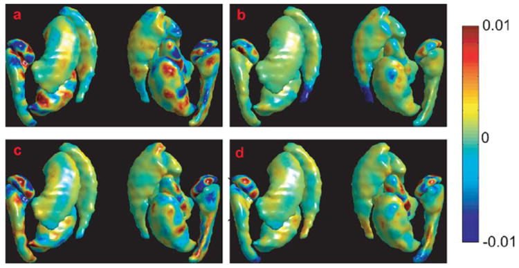
Panels (a)–(d), respectively, show the first four principal components of the initial momentum on the template surface of the subcortical structures. The lateral and medial views are, respectively, illustrated on the left and right sidesof each panel.

Fig. 2.

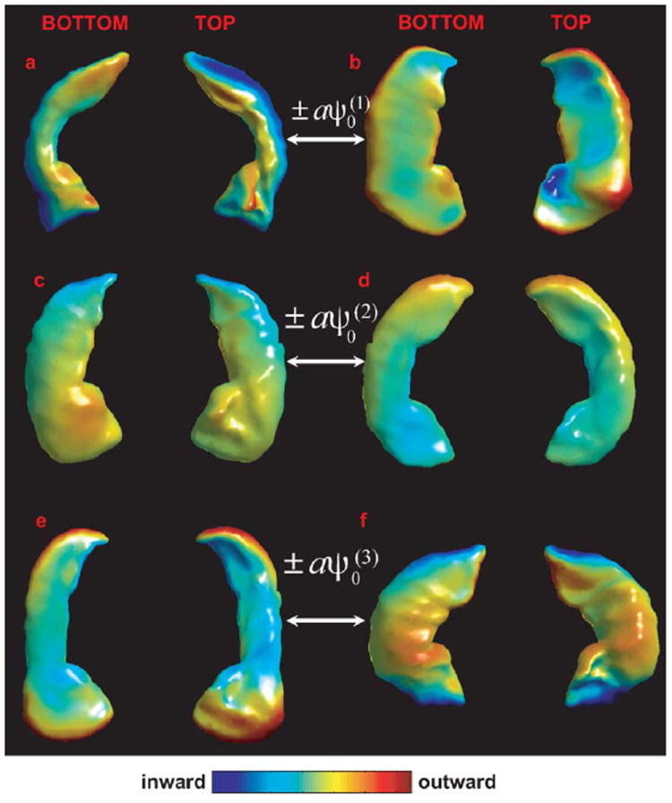
Three rows show geodesic shooting of the initial momentum using the first three principal components, ± $a{\psi }_0^{(k)}$, k = 1, 2, 3, a > 0, respectively. The left and right columns in each row represent hippocampal shapes synthesized at −20 ${\psi }_0^{(k)}$ and 20 ${\psi }_0^{(k)}$, respectively. Regions with outward and inward deformations are, respectively, colored in red and blue.

Fig. 3.

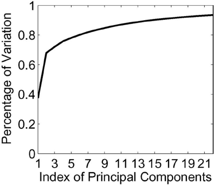
The cumulative distribution of shape variations contributed by the first 22 principal components.

A. Stability of the Eigenspace

Since the eigenspace of the initial momentum was constructed using the data-driven PCA approach, it is altered when training samples are changed. In order to evaluate the stability of the eigenspaces with respect to changes in the composition of the training samples, we calculated a set of principal canonical angles and the chordal distance between two eigenspaces with respect to the metric defined in (8) [29]. Considering two eigenspaces with respective generative families $\mathrm{\Psi }=\{{\psi }_0^{(1)},{\psi }_0^{(2)},\dots ,{\psi }_0^{(p)}\}$ and $\stackrel{\sim }{\mathrm{\Psi }}=\{{\stackrel{\sim }{\psi }}_0^{(1)},{\stackrel{\sim }{\psi }}_0^{(2)},\dots ,{\stackrel{\sim }{\psi }}_0^{(p)}\}$. We applied a singular value decomposition (SVD) algorithm [30] for computing cosines of principal angles. The reduced SVD of 〈Ψ, k_V Ψ̃〉₂ is

$$U^{\ast }{\mathrm{\Psi }}^{\ast }{k}_V\stackrel{\sim }{\mathrm{\Psi }}V=\mathit{diag}({\sigma }_1,{\sigma }_2,\dots ,{\sigma }_p,1\ge {\sigma }_1\ge {\sigma }_2,\dots \ge {\sigma }_p\ge 0$$

where U and V are unitary matrices. Then the principal angles and chordal distance can be, respectively, computed as θ_i = arccos(σ_i), i = 1, 2, …, p, and $d_p(\mathrm{\Psi },\stackrel{\sim }{\mathrm{\Psi }})=\sqrt{{\sum }_{i=1}^p{\sin }^2({\theta }_i)}$. The larger θ_p and d_p, the more unstable the eigenspace with rank p.

In our experiment, we employed a bootstrapping procedure for randomly extracting a sample of 166 subcortical surfaces from the training set for 10 000 times. In each sample, a new eigenspace was computed. The principal angles between the new eigenspace and the eigenspace based on the entire training set are computed. Fig. 4(a) shows the mean and standard deviation of the first 22 principal angles among all 10 000 bootstrapped samples. This indicates that the first 10 principal angles are less than 10° and account for 85% of the shape variations among the 166 subjects (see Fig. 3). As illustrated in Fig. 4(b), the chordal distance between the two eigenspaces constructed by the first 10 PCs is less than 0.30. Thus, the eigenspace constructed by the first 10 PCs were used in the PCDM-surface algorithm throughout the rest of the experiments in this paper.

Fig. 4.

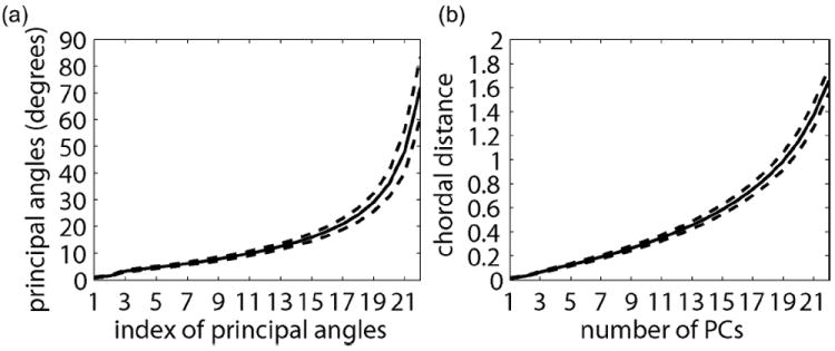
Panels (a) and (b), respectively, show the first 22 principal angles and the chordal distance between the eigenspace of the 166 training sets and those computed based on the boot-strapped samples. The solid and dashed curves, respectively, represents the mean and standard deviation among all 10 000 boot-strapped samples.

B. Registration Accuracy

We validated the mapping accuracy of the PCDM-surface algorithm for the hippocampus when small alterations of the prior law were considered. This was done in a leave-one-out fashion. During each mapping, 165 out of total 166 hippocampal surfaces were selected as training sets and used to compute the eigenspace of the initial momentum. Then, the remaining one hippocampus was considered as a new observable surface which the hippocampal template surface is registered to. We repeated this for 166 times.

We computed a surface distance graph defined as the percentage of vertices on the deformed template surface having the distance to subject’s surface less than d mm. Since the surface distance is not used in our mapping functional J and the hippocampal shape is globular, it is a reasonable measure for quantifying the accuracy of the mapping. Fig. 5 shows the surface distance graphs for individual hippocampal surfaces (grey lines) and their average (black line), which indicates in average about 95% of the vertices on the deformed template surfaces have the distance to the subject’s surface less than 1 mm, the resolution of the MR images.

Fig. 5.

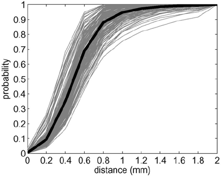
Surface distance graphs are shown to quantify the percentage of vertices on the deformed template surface having the distance to subject’s surface less than d mm. Grey lines are the surface distance graphs of individual hippocampal surfaces. Black line represents the surface distance graph averaged among all 166 hippocampal surfaces.

C. Robustness of the PCDM-Surface Algorithm to Unseen Shapes

We tested the robustness of the PCDM-surface algorithm using 10 hippocampal surfaces of patients with Alzheimer’s disease (AD) (age: 71.1 ± 3.2; MMSE: 19.8 ± 3.7) when the 166 healthy subjects were used to compute the eigenspace. We chose this example because it is well known that effects of healthy aging and AD processes on the hippocampus are distinct as suggested by literature [31]. Beyond the aging effects on the hippocampal volume reduction, hippocampal shape compression is particularly observed in the subiculum (the inferior aspect of the hippocampus) and then in CA1 (the lateral aspect of the hippocampus) during the AD progression. We thus expected that the hippocampal shapes of AD patients cannot be fully characterized by the eigenspace obtained from the healthy population no matter regardless the size of training samples. Hence, our example showing here can demonstrate the robustness of the PCDM-surface algorithm to unseen shapes.

Fig. 6 illustrates the mean surface distance graphs between the template surface and the patients’ surfaces before (black) and after the PCDM mapping (red). This indicates that in average about 95% of the vertices on the deformed template surfaces have the distance to the surfaces of the 10 AD patients less than 1 mm, while only 70% of the vertices on the template surface have the distance to the surfaces of the AD patients less than 1 mm. We perform a one-sided Kolmogorov–Smirnov (KS) test on the surface distance graph and hypothesize that there is no difference in the distance measure before or after the PCDM mapping against the alternative that the mapping significantly improved the hippocampal alignment. The distribution of KS statistics is empirically estimated using the permutation-based resampling approach. The resampling was performed by randomly labeling the surface distance graph as obtained from before or after the surface mapping. The KS statistic was recomputed for each resampled dataset. By repeating this process ten thousand times, an empirical null distribution of the KS statistic was constructed, and the p-value was computed as a percentage of the KS statistics greater than the KS value from the original dataset. The KS test revealed that the distance between the deformed template and the surfaces of the AD patients was significantly smaller than that before the mapping (p < 0.0001), suggesting the robustness of the PCDM-surface algorithm for the cases when anatomies were not included for constructing the eigenspace of the initial momenta.

Fig. 6.

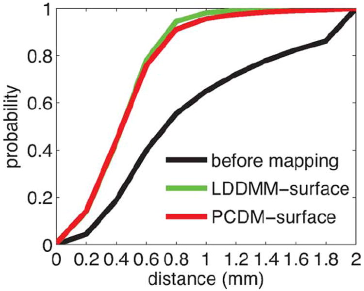
Surface distance graphs are shown to quantify the percentage of vertices on the deformed template surface having the distance to subject’s surface less than d mm. Black, green, and red curves are the average surface distance graphs across 10 Alzheimer’s disease patients before and after the LDDMM-surface and PCDM mappings, respectively.

We also compared these PCDM-surface mapping results with those obtained using the previous LDDMM-surface mapping algorithm [15]. The green curve in Fig. 6 shows the average surface distance graph between the surfaces of the AD patients and the template surface deformed by the LDDMM-surface algorithm [15]. The KS test suggested that the performance of the PCDM-surface mapping is comparable to that of the LDDMM-surface mapping [15] (p = 0.9) even though the anatomies of the AD patients were not incorporated in the training samples.

IV. Conclusion

We introduce a diffeomorphic metric mapping algorithm that directly incorporates the empirical shape prior model of the initial momentum in the LDDMM framework, which has never been done before. We provide a simple and effective algorithm for computing the shape prior model using PCA and a gradient descent algorithm that estimates a set of coefficients associated with the eigenfunctions of the initial momentum defined at the template coordinates. Unlike previous LDDMM algorithms [14], [15], the PCDM-surface mapping reduces the dimensionality of diffeomorphic deformation and thus directly provides the succinct representation of shapes for shape classification and atlas estimation. Moreover, our experiments demonstrate that the method is not sensitive to the eigenspace constructed based on the training set but robust against shape variations that are not observed in the training set.

In this paper, we optimize the set of coefficients associated with the PCs of the initial momentum using the gradient descent, which is similar to that in [15] with the additional computation of the inner product between the PCs and η_t^α. Thus, the computational cost of the PCDM algorithm proposed in this paper is the same as previous LDDMM algorithms [15]. However, our approach using a shape prior potentially leads to a future fast computation algorithm for the diffeomorphic mapping. As mentioned in the experiments, only few scalar coefficients need to be estimated given the eigenspace of the initial momentum. This gives opportunities to employ Monte Carlo or brute-force search methods for seeking optimal coefficients associated with shape eigenfunctions and thus speed up the optimization of the diffeomorphic mapping, which cannot be accomplished in the previous diffeomorphic mapping algorithms [14]-[16]. We will employ different numerical schemes for future research.

We notice a potential limitation of our work, that is, the PCDM-surface mapping algorithm is a template dependent approach. In our discussion of both methodology and results, we consider that the template is known and fixed. According to the conservation law of momentum, the initial momenta of individual shapes must be defined in a fixed template coordinate such that they can be in a linear space to facilitate the computation of their eigenspace using PCA. Nevertheless, this is also one of the strengths for representing random shapes using initial momenta, which allows using simple linear statistical methods to model complex nonlinear diffeomorphisms. Due to this fact, we chose the averaged shape computed based on the manual labeled subcortical structures of forty subjects as template in our experiments [28]. Our template is centered among the training samples in terms of its diffeomorphic metric distance to the training samples (see more discussion in [28]), which gives a reasonable starting point for the PCDM-surface mapping algorithm. Further investigation of the influences of the template on the eigenspace of the initial momentum and the surface mapping accuracy is needed.

References

- 1.Qiu A, Crocetti D, Adler M, Mahone M, Deckla M, Miller MI, Mostofsy SH. Basal ganglia volume and shape in children with ADHD. Am J Psychiatry. 2009;166(no. 1):74–82. doi: 10.1176/appi.ajp.2008.08030426. [DOI] [PMC free article] [PubMed] [Google Scholar]
- 2.Narr KL, Thompson PM, Sharma T, Moussai J, Zoumalan C, Rayman J, Toga AW. Three-dimensional mapping of gyral shape and cortical surface asymmetries in schizophrenia: Gender effects. Am J Psychiatry. 2001;158:244–255. doi: 10.1176/appi.ajp.158.2.244. [DOI] [PMC free article] [PubMed] [Google Scholar]
- 3.Apostolova L, Morra J, Green A, Hwang K, Avedissian C, Woo E, Cummings J, Toga A, Jack CJ, Weiner M, Thompson P, Initiative ADN. Automated 3d mapping of baseline and 12-month associations between three verbal memory measures and hippocampal atrophy in 490 ADNI subjects. Neuroimage. 2010;51:488–499. doi: 10.1016/j.neuroimage.2009.12.125. [DOI] [PMC free article] [PubMed] [Google Scholar]
- 4.Davies R, Twining C, Cootes T. A minimum description length approach to statistical shape modeling. IEEE Trans Med Imag. 2002 May;21(no. 5):525–537. doi: 10.1109/TMI.2002.1009388. [DOI] [PubMed] [Google Scholar]
- 5.Hufnagel H, Pennec X, Ehrhardt J, Handels H, Ayache N, Ayache N, Ourselin S, Maeder A, editors. Proc Med Image Computing Computer Assist Intervent (MICCAI’07) Vol. 4791. Brisbane, Australia: LNCS; Oct, 2007. Shape analysis using a point-based statistical shape model built on correspondence probabilities; pp. 959–967. [DOI] [PubMed] [Google Scholar]
- 6.Fischl B, Sereno MI, Tootell RBH, Dale AM. High-resolution inter-subject averaging and a surface-based coordinate system. Hum Brain Mapp. 1999;8:272–284. doi: 10.1002/(SICI)1097-0193(1999)8:4<272::AID-HBM10>3.0.CO;2-4. [DOI] [PMC free article] [PubMed] [Google Scholar]
- 7.Robbins S, Evans A, Collins D, Whitesides S. Tuning and comparing spatial normalization methods. Med Image Anal. 2004;8:311–323. doi: 10.1016/j.media.2004.06.009. [DOI] [PubMed] [Google Scholar]
- 8.Wang Y, Gu X, Hayashi KM, Chan TF, Thompson PM, Yau S-T. Surface parameterization using Riemann surface structure. ICCV. 2005:1061–1066. doi: 10.1007/11566489_81. [DOI] [PubMed] [Google Scholar]
- 9.Chung M, Qiu A, Nacewicz B, Pollak S, Davidson R, Pennec X, Joshi S, editors. Tiling manifolds with orthonormal basis. Foundations Computat Anat; Proc MICCAI 2008 Workshop Math; New York: 2008. pp. 128–139. [Google Scholar]
- 10.Chung M, Dalton K, Davidson R. Tensor-based cortical surface morphometry via weighed spherical harmonic representation. IEEE Trans Med Imag. 2008 Aug;27(no. 8):1143–1151. doi: 10.1109/TMI.2008.918338. [DOI] [PubMed] [Google Scholar]
- 11.Yu P, Grant P, Qi Y, Han X, Ségonne F, Pienaar R, Busa E, Pacheco J, Makris N, Buckner RL, Golland P, Fischl B. Cortical surface shape analysis based on spherical wavelets. IEEE Trans Med Imag. 2007 Apr;26(no. 4):582–597. doi: 10.1109/TMI.2007.892499. [DOI] [PMC free article] [PubMed] [Google Scholar]
- 12.Nain D, Haker S, Bobick A, Tannenbaum A. Multiscale 3D shape analysis using spherical wavelets. MICCAI. 2005:459–467. doi: 10.1007/11566489_57. [DOI] [PMC free article] [PubMed] [Google Scholar]
- 13.Nain D, Styner M, Niethammer M, Levitt J, Shenton M, Gerig G, Bobick A, Tannenbaum A. Statistical shape analysis of brain structures using spherical wavelets. Proc 4th IEEE Int Symp Biomed Imag : From Nano to Macro. 2007:209–212. doi: 10.1109/isbi.2007.356825. [DOI] [PMC free article] [PubMed] [Google Scholar]
- 14.Vaillant M, Glaunès J. Surface matching via currents. Inform Proc in Med Imag. 2005;3565:381–392. doi: 10.1007/11505730_32. Lecture Notes Comp. Sci. [DOI] [PubMed] [Google Scholar]
- 15.Zhong J, Qiu A. Multi-manifold diffeomorphic metric mapping for aligning cortical hemispheric surfaces. NeuroImage. 2010;49:355–365. doi: 10.1016/j.neuroimage.2009.08.026. [DOI] [PubMed] [Google Scholar]
- 16.Durrleman S, Pennec X, Trouvé A, Ayache N. Statistical models on sets of curves and surfaces based on currents. Med Image Anal. 2009;13:793–808. doi: 10.1016/j.media.2009.07.007. [DOI] [PubMed] [Google Scholar]
- 17.Miller MI, Trouvé A, Younes L. Geodesic shooting for computational anatomy. J Math Imag Vis. 2006;24:209–228. doi: 10.1007/s10851-005-3624-0. [DOI] [PMC free article] [PubMed] [Google Scholar]
- 18.Vaillant M, Miller MI, Younes L, Trouvé A. Statistics on diffeomorphisms via tangent space representations. NeuroImage. 2004;23:161–169. doi: 10.1016/j.neuroimage.2004.07.023. [DOI] [PubMed] [Google Scholar]
- 19.Wang L, Beg MF, Ratnanather JT, Ceritoglu C, Younes L, Morris JC, Csernansky JG, Miller MI. Large deformation diffeomorphism and momentum based hippocampal shape discrimination in dementia of the alzheimer type. IEEE Trans Med Imag. 2007 Apr;26(no. 4):462–470. doi: 10.1109/TMI.2005.853923. [DOI] [PMC free article] [PubMed] [Google Scholar]
- 20.Grenander U, Miller MI. Computational anatomy: An emerging discipline. Q App Math. 1998;56(no. 4):617–694. [Google Scholar]
- 21.Dupuis P, Grenander U, Miller MI. Variational problems on flows of diffeomorphisms for image matching. Q Appl Math. 1998;56:587–600. [Google Scholar]
- 22.Trouvé A. Diffeomorphism groups and pattern matching in image analysis. Int J Comp Vis. 1998;28(no. 3):213–221. [Google Scholar]
- 23.Vaillant M, Qiu A, Glaunès J, Miller MI. Diffeomorphic metric surface mapping in subregion of the superior temporal gyrus. NeuroImage. 2007;34:1149–1159. doi: 10.1016/j.neuroimage.2006.08.053. [DOI] [PMC free article] [PubMed] [Google Scholar]
- 24.Yang C, Duraiswami R, Gumerov N, Davis L. Improved fast gauss transform and efficient kernel density estimation. IEEE Int Conf Comput Vis. 2003:464–471. [Google Scholar]
- 25.Marcus DS, Wang TH, Parker J, Csernansky JG, Morris JC, Buckner RL. Open access series of imaging studies (oasis): Cross-sectional MRI data in young, middle aged, nondemented, and demented older adults. J Cogn Neurosci. 2007;19:1498–1507. doi: 10.1162/jocn.2007.19.9.1498. [DOI] [PubMed] [Google Scholar]
- 26.Fischl B, Salat DH, Busa E, Albert M, Dieterich M, Haselgrove C, van der Kouwe A, Killiany R, Kennedy D, Klaveness S, Montillo A, Makris N, Rosen B, Dale AM. Whole brain segmentation: Automated labeling of neuroanatomical structures in the human brain. Neuron. 2002;33:341–355. doi: 10.1016/s0896-6273(02)00569-x. [DOI] [PubMed] [Google Scholar]
- 27.Qiu A, Miller MI. Multi-structure network shape analysis via normal surface momentum maps. NeuroImage. 2008;42:1430–1438. doi: 10.1016/j.neuroimage.2008.04.257. [DOI] [PubMed] [Google Scholar]
- 28.Qiu A, Brown T, Fischl B, Ma J, Miller MI. Atlas generation of subcortical and ventricular structures with its applications in shape analysis. IEEE Trans Image Process. 2010 Jun;19(no. 6):1539–1547. doi: 10.1109/TIP.2010.2042099. [DOI] [PMC free article] [PubMed] [Google Scholar]
- 29.Bjorck A, Golub GH. Numerical methods for computing angles between linear subspaces. Math Comp. 1973;27:579–594. [Google Scholar]
- 30.Golub GH, Loan CFV. Matrix Computations. third. Baltimore, MD: Johns Hopkins Univ Press; 1996. [Google Scholar]
- 31.Csernansky JC, Wang L, Joshi S, Miller JP, Gado M, Kido D, McKeel D, Morris J, Miller M. Early DAT is distinguished from aging by high dimensional mapping of the hippocampus. Neurology. 2000;55:1636–1643. doi: 10.1212/wnl.55.11.1636. [DOI] [PubMed] [Google Scholar]