Feature-preserving surface mesh smoothing via suboptimal Delaunay triangulation

Abstract

A method of triangular surface mesh smoothing is presented to improve angle quality by extending the original optimal Delaunay triangulation (ODT) to surface meshes. The mesh quality is improved by solving a quadratic optimization problem that minimizes the approximated interpolation error between a parabolic function and its piecewise linear interpolation defined on the mesh. A suboptimal problem is derived to guarantee a unique, analytic solution that is significantly faster with little loss in accuracy as compared to the optimal one. In addition to the quality-improving capability, the proposed method has been adapted to remove noise while faithfully preserving sharp features such as edges and corners of a mesh. Numerous experiments are included to demonstrate the performance of the method.

1. Introduction

Triangular surface meshes are widely used in computer graphics, industrial design and scientific computing. In computer graphics and design, people are typically interested in the smoothness (low variation in curvature) and sharp features (edges, corners, etc.) of a mesh. In many applications of scientific computing, however, the quality of a mesh is a key factor that significantly affects the numerical result of finite or boundary element analysis. One of the most common criteria for mesh quality is the uniformity of angles, although this may not be the best in some cases where anisotropic meshes are desired [1]. For its popularity, however, we shall adopt the angle-based criterion in the present work. In many real applications, the input meshes often have low quality, containing angles close or even equal to 0° or 180°. The main interest and contribution of the present work is to improve the quality of triangular surface meshes. Additionally our method will be extended to be able to remove noise and preserve sharp features on surface meshes. For simplicity, we refer to both mesh quality improvement and mesh denoising as mesh smoothing unless otherwise specified.

Mesh denoising has a long history in computer graphics and the related methods include three main categories: (1) geometric flows [2-6], (2) spectral analysis [7,8], and (3) optimization methods [9,10]. Due to its simplicity and low computational cost, Laplacian smoothing has established itself as one of the most common methods among all the geometric flow-based methods. In this method, every node is updated towards the barycenter of the neighborhood of the node. However, volume shrinkage often occurs during this process. The shrinkage problem may be tackled by methods utilizing spectral analysis of the mesh signal, which is the main idea of the second category. Optimization-based methods guarantee the smoothness of the mesh by minimizing different types of energy functions. But the iterative process searching for optimal solutions can be time-consuming.

A variety of techniques on mesh quality improvement have been developed [11,12]. Some of the existing techniques include: (1) inserting/deleting vertices [13], (2) swapping edges/faces [14], (3) remeshing [15-18], and (4) moving vertices without changing mesh topology [19-22]. Two or more of the above techniques are sometimes combined to achieve better performance. For instance, Dyer et al. [23] integrate edge flipping, remeshing and decimation into one framework for generating high-quality Delaunay meshes. In the current work, however, we shall restrict ourselves to the methods in the last category that only adjust the nodes’ coordinates. Among these methods, Laplacian smoothing in its simplest form that moves a vertex to the center or barycenter of the surrounding vertices [19] is one of the fastest methods but it may fail in improving mesh quality and is often equipped with other techniques such as optimizations [24,25]. Ohtake et al. [26] presented a method of simultaneously improving and denoising a mesh based on a combination of mean curvature flow and Laplacian smoothing. Nealen et al. [27] introduced a framework for mesh improving and denoising using Laplacian-based least-squares techniques. Both methods, as shown in [28], cannot warrant mesh quality or feature-preservation. Wang et al. [28] presented a method for mesh denoising and quality improvement by local surface fitting and maximum inscribed circles but it was heuristic and lacked mathematical foundations.

Among all the repositioning-based methods for mesh quality improvement, the optimal Delaunay triangulation (ODT) [29,1,30] has been proved to be effective on 2D triangular meshes. However, the extension from 2D meshes to 3D surface meshes is non-trivial in both mathematical analysis and algorithm design. For 3D surface meshes we need to consider not only angle quality but also mesh noise that causes bumpiness on surfaces, which was not taken into account in the original ODT method or its variants in tetrahedral mesh smoothing [31,32]. In addition, sharp surface features must be well preserved during the processes of mesh denoising and quality improvement. There have been extensive studies on feature-preserving surface mesh processing [33-38]. However, most of the previous work was focused on the mesh denoising problem but only a few dealt with both mesh denoising and quality improvement with feature preservation [28].

The main goal of the present paper is to generalize the 2D ODT idea to 2-manifold surface meshes by formulating the mesh quality improvement as an optimization problem that minimizes the interpolation error between a parabolic function and its piecewise linear interpolation at each vertex of the surface mesh. Unfortunately there is no analytical solution to this optimization problem. To solve the minimization problem faster, we consider a suboptimal problem by simplifying the objective function into a quadratic formula such that an analytical solution can be derived. The proposed suboptimal Delaunay triangulation (or S-ODT) is then extended to include two other capabilities: removing mesh noise as well as preserving sharp features on the original meshes. These two goals are achieved by using two standard techniques: curve/surface fitting [39] and local structure tensors [33].

The remainder of this paper is organized as follows. In Section 2, we extend the original ODT method [29,1] to improve the angle quality of a surface mesh. Several variants of the new algorithm are also introduced to warrant additional desirable properties such as noise removal and feature preservation. Numerous mesh examples are included and comparisons are given in Section 3 to demonstrate the performance of the proposed algorithms, followed by our conclusions in Section 4. Some mathematical details of the algorithms are provided in the Appendices.

2. Method

Like many other mesh smoothing approaches, our method is iterative and vertex-based, meaning that all mesh vertices are repositioned in each iteration and the process is repeated until the mesh quality meets some predefined criteria or a maximum number of iterations is reached. In this section we shall describe three algorithms with the basic one addressing the mesh quality improvement using the proposed sub-optimization formulation and two extended algorithms dealing additionally with the issues of feature preservation and noise removal. For completeness, we shall begin with a brief introduction to Delaunay triangulation and the original ODT method [29]. More details on ODT-based 2D/3D and local/global mesh smoothing algorithms can be found in [1,30].

2.1. Brief introduction to ODT

In computational geometry, Delaunay triangulation (DT) is a well known scheme to triangulate a finite set of fixed points P, satisfying the so-called empty sphere condition. That is, no point in P can be inside the circumsphere of any simplex (e.g., triangle) in DT(P). Consider, for example, the four points p0, p1, p2 and p3 in Fig. 1a and b. There are obviously two ways to triangulate this point set, but only the one in Fig. 1b is a Delaunay triangulation that produces a larger minimum angle than that in Fig. 1a and thus is preferable according to the angle-based criterion. Fig. 1a and b also tells us another interpretation of Delaunay triangulation. If we lift the point set onto a parabolic function ||x||², any triangulation on the lifting points q0,q1,q2 and q3 will result in a unique piecewise linear interpolation of the parabolic function. The one that minimizes the interpolation error can be projected back to the original point set and makes the Delaunay triangulation. From this example, we can see that Delaunay triangulation of a fixed point set is equivalent to minimizing the following interpolation error, which can be achieved by swapping edges:

$$Q(DT,\mid \mid \mathbf{x}\mid {\mid }^2,q)=\underset{\mathcal{T}\in {\mathcal{T}}_p}{\min }Q(\mathcal{T},\mid \mid \mathbf{x}\mid {\mid }^2,q),\forall 1\le q\le \infty ,$$ (1)

where $Q(\mathcal{T},\mid \mid \mathbf{x}\mid {\mid }^2,q)$ is the L^q distance between the parabolic function ||x||² and its piecewise linear interpolation $\mid \mid \mathbf{x}\mid {\mid }_I^2$ based on a particular triangulation $\mathcal{T}$ of a fixed point set P. ${\mathcal{T}}_p$ is the set of all possible triangulations of P.

Fig. 1.

Illustration of minimizing interpolation error in two ways: edge swapping (a and b) and vertex-repositioning (c and d). The mesh quality in (b) is improved by swapping the edges but keeping the vertices fixed. The interpolation error can also be reduced (hence mesh quality is improved) by moving the vertex p0 in (c) to a new position in (d), where the edge connections are kept unchanged.

Although Delaunay triangulation is optimal for a fixed set of points, it does not necessarily produce a high quality mesh if the given points are not nicely distributed. In addition to edge-swapping, there is actually another way, called vertex-repositioning, to minimize the error between a parabolic function and its piecewise linear interpolation. Consider for example the point set in Fig. 1c. The triangulation is already optimal in terms of the DT criterion. However, the interpolation error can be further reduced by moving the vertex p0 to a better position as shown in Fig. 1d and hence the mesh quality is improved. This strategy constitutes the core of the optimal Delaunay triangulation (ODT) method as detailed in [1,29,30].

It is worth noting that the vertex-repositioning alone does not produce a Delaunay-like triangulation. For better mesh quality improvement, it is always wise to combine edge-swapping into vertex-repositioning, as in the original ODT method [29]. In the rest of the current paper, we shall extend the ODT method to surface meshes to improve the angle quality. However, we will not consider the edge-swapping technique in the descriptions of our algorithms as well as results, simply because our main focus in the current paper is how vertices are repositioned to achieve quality improvement and two other goals (noise removal and feature preservation).

2.2. Optimal Delaunay triangulation on surfaces

Suppose $\mathcal{M}$ is a triangular surface mesh in ${\mathbb{R}}^3$ and the sets of vertices (or nodes) and faces are $\mathcal{V}$ and $\mathcal{K}$ respectively. Let x_* be the optimal position of a Vertex ${\mathbf{x}}_0\in \mathcal{V}$ in the sense that the following interpolation error is minimized:

$$\begin{array}{cc}\hfill E\left({\mathbf{x}}^{\prime }\right)=& {\int }_{\mathbf{x}\in {\mathcal{N}}^{\prime }}\mid f_I(\mathbf{x}-{\mathbf{x}}^{\prime })-f(\mathbf{x}-{\mathbf{x}}^{\prime })\mid \mathrm{d}\mathbf{x}\hfill \\ \hfill =& \sum _{k=1}^N{\int }_{\mathbf{x}\in {\tau }_k^{\prime }}{f}_I(\mathbf{x}-{\mathbf{x}}^{\prime })-f(\mathbf{x}-{\mathbf{x}}^{\prime })\mathrm{d}\mathbf{x},\hfill \end{array}$$ (2)

where x′ is the varying (new) position of x₀, ${\mathcal{N}}^{\prime }\subset \mathcal{K}$ is the set of N neighboring triangles around x′, f(x) = ||x||² is a parabolic function in ${\mathbb{R}}^3$; f_I(x) the piecewise linear interpolation of f(x) based on ${\mathcal{N}}^{\prime }$, and ${\tau }_k^{\prime }$ is the kth triangle in ${\mathcal{N}}^{\prime }$. Note that f_I(x) is always no less than f(x) so that we can remove the absolute-value operation in the first equation of (2).

The key of minimizing (2) is to compute the sum of the surface integrals in all the neighboring triangles around x′. Suppose ${\tau }_k^{\prime }$ is formed by 〈x′, x_k, x_k+1〉 (let x_N+1 = x₁), the integral ${\int }_{x\in {\tau }_k^{\prime }}{f}_I(\mathbf{x}-{\mathbf{x}}^{\prime })-f(\mathbf{x}-{\mathbf{x}}^{\prime })\mathrm{d}\mathbf{x}$ can be computed by replacing x with x′+ λ₁(x_k − x′) + λ₂(x_k+1 − x′), where λ₁, λ₂ ≥ 0 and λ₁ + λ₂ ≤ 1. Thus (2) becomes the following equation (see A for details):

$$E\left({\mathbf{x}}^{\prime }\right)=\sum _{k=1}^N[{({\mathbf{x}}_k-{\mathbf{x}}^{\prime })}^2+{({\mathbf{x}}_{k+1}-{\mathbf{x}}_k)}^2{({\mathbf{x}}_{k+1}-{\mathbf{x}}_k)}^2]{\mathcal{S}}_k^{\prime },$$ (3)

where ${\mathcal{S}}_k^{\prime }$ is the area of ${\tau }_k^{\prime }$. Note that ${\mathcal{S}}_k^{\prime }$ depends on x′ introducing additional non-linearity to the error function.

The minimizer of (3) in general does not admit a closed-form expression. Although numerical methods may be used for solving (3), it can be computationally inefficient, as will be demonstrated in Section 3. For this reason, we shall take another strategy by replacing ${\mathcal{S}}_k^{\prime }$ with other types of weights, yielding a suboptimal problem that can be analytically and more efficiently solved. The simplest case is that, if we set ${\mathcal{S}}_k^{\prime }\equiv 1$ for k = 1, 2, …, N, the solution of (3) is equivalent to the Laplacian smoothing that moves x′ towards the barycenter of its neighborhood in $\mathcal{K}$. Therefore, Laplacian smoothing is just a special case of (3).

2.3. Suboptimal Delaunay triangulation on surfaces

In this work, we replace each ${\mathcal{S}}_k^{\prime }$ in (3) with ${\mathrm{D}}_k^{\prime }=\det ({\mathbf{x}}_k-{\mathbf{x}}^{\prime },{\mathbf{x}}_{k+1}-{\mathbf{x}}^{\prime },\mathbf{n})$, where n is the unit normal vector of a plane Π_t on which x′ is allowed to move. As an approximation to the tangent plane at x₀, Π_t is computed as follows:

$$\mathbf{n}=\frac{{\Sigma }_{k=1}^N{\mathcal{S}}_k{\mathbf{n}}_k}{\mid \mid {\Sigma }_{k=1}^N{\mathcal{S}}_k{\mathbf{n}}_k\mid \mid },$$ (4)

where ${\mathcal{S}}_k$ and n_k are the area and unit normal vector of the kth neighboring triangle of x₀ in the original mesh. As shown in D, when x′ is restricted to the tangent plane defined this way, the volume of a closed mesh can be exactly preserved. Please note that at this moment, we assume that the original mesh is smooth enough and noise-free, such that the tangent plane is well defined as above. For meshes with sharp features or noise, special care must be taken to calculate tangent planes (or feature lines) as will be discussed in the subsequent subsections. In these cases, the volume preservation is not guaranteed.

Note that ${\mathrm{D}}_k^{\prime }$ is the area of the projection of ${\tau }_k^{\prime }$ onto Π_t, the ratio between any two ${\mathrm{D}}_k^{\prime }$’s is a good approximation of the ratio between the two corresponding ${\mathcal{S}}_k^{\prime }$’s. With this in mind, we replace each ${\mathcal{S}}_k^{\prime }$ in (3) with ${\mathrm{D}}_k^{\prime }$ and have the following approximated, suboptimal Delaunay triangulation (S-ODT) problem:

$$\begin{array}{cc}\hfill {\mathbf{x}}_{\ast }=& \mathrm{argmin}\stackrel{‒}{E}\left({\mathbf{x}}^{\prime }\right)\text{with}\hfill \\ \hfill \stackrel{‒}{E}\left({\mathbf{x}}^{\prime }\right)& =\sum _{k=1}^N[{({\mathbf{x}}_k-{\mathbf{x}}^{\prime })}^2+{({\mathbf{x}}_{k+1}-{\mathbf{x}}_k)}^2{({\mathbf{x}}_{k+1}-{\mathbf{x}}_k)}^2]{\mathrm{D}}_k^{\prime }.\hfill \end{array}$$ (5)

We shall see in Section 3, especially Fig. 6, that the approximation of ${\mathrm{S}}_k^{\prime }$ with ${\mathrm{D}}_k^{\prime }$ makes sense (i.e., with significantly less computational time but little loss in mesh quality).

Fig. 6.

Performance comparison between the analytical solution to the suboptimal problem (the proposed S-ODT method: Algorithm 1) and the numerical solution to the optimal problem (Eq. (3)). (a) The original RyR mesh. (b–d) Show respectively the angle histograms of the original mesh, the mesh smoothed by the S-ODT method, and the mesh smoothed by the numerically-based ODT method. (e–g) Show a closer look at the three meshes respectively. While little difference is observed between the two smoothed meshes, the computational time is only about 36 s by using the analytical method for 20 iterations, in contrast to 1 min and 56 s by using the L-BFGS method for five iterations.

As each ${\mathrm{D}}_k^{\prime }$ also has linear dependence on x′, the error $\stackrel{‒}{E}$ seems to have cubic dependence on x′ and thus the minimizer of (5) does not seem to admit a closed form expression. Fortunately, the sum of all ${\mathrm{D}}_k^{\prime }$ is a constant (i.e., ${\Sigma }_{k=1}^N{\mathrm{D}}_k^{\prime }\equiv C$; see B for the proof) if all the neighbors around x′ are fixed (i.e., we smooth the mesh locally). This property makes the sum of all cubic terms in (5) a constant and thus minimizing (5) becomes an unconstrained quadratic optimization problem such that an analytic solution can be obtained.

In order to preserve the local shape (and volume too) of the original mesh near x′, we restrict x′ to moving only in the tangent plane Π_t. Thus x′ in (5) can be written as a parametric representation as follows:

$${\mathbf{x}}^{\prime }={\mathbf{x}}_0+u\mathbf{s}+v\mathbf{t},$$ (6)

where s and t are two orthogonal unit vectors on Π_t, and u, v are the coordinates of x′ corresponding to s and t respectively.

Algorithmically the optimal coordinates u_*, v_* can be computed by solving the following system of linear equations:

$$\left(\begin{array}{cc}\hfill 2\epsilon \hfill & \hfill \mathcal{G}\hfill \\ \hfill \mathcal{G}\hfill & \hfill 2\mathcal{F}\hfill \end{array}\right)\left(\begin{array}{c}\hfill u\hfill \\ \hfill v\hfill \end{array}\right)=\left(\begin{array}{c}\hfill \mathcal{H}\hfill \\ \hfill \mathcal{I}\hfill \end{array}\right)$$ (7)

where $\epsilon ,\mathcal{F},\mathcal{G},\mathcal{H},\mathcal{I}$ are determined in the following way:

$$\{\begin{array}{c}\epsilon =C+\sum _{k=1}^N\left[\mathbf{s}\right({\mathbf{X}}_k+{\mathbf{X}}_{k+1}\left)\det \right(\mathbf{s},{\mathbf{X}}_{k+1}-{\mathbf{X}}_k,\mathbf{n}\left)\right]\hfill \\ \mathcal{F}=C+\sum _{k=1}^N\left[\mathbf{t}\right({\mathbf{X}}_k+{\mathbf{X}}_{k+1}\left)\det \right(\mathbf{t},{\mathbf{X}}_{k+1}-{\mathbf{X}}_k,\mathbf{n}\left)\right]\hfill \\ \mathcal{G}=\sum _{k=1}^N\left[\mathbf{s}\right({\mathbf{X}}_k+{\mathbf{X}}_{k+1}\left)\det \right(\mathbf{t},{\mathbf{X}}_{k+1}-{\mathbf{X}}_k,\mathbf{n})+\mathbf{t}({\mathbf{X}}_k+{\mathbf{X}}_{k+1}\left)\det \right(\mathbf{s},{\mathbf{X}}_{k+1}-{\mathbf{X}}_k,\mathbf{n}\left)\right]\hfill \\ \mathcal{H}=\sum _{k=1}^N\left[\mathbf{s}\right({\mathbf{X}}_k+{\mathbf{X}}_{k+1}\left)\det \right({\mathbf{X}}_k,{\mathbf{X}}_{k+1},\mathbf{n})+({\mathbf{X}}_k^2+{\mathbf{X}}_{k+1}^2-{\mathbf{X}}_k{\mathbf{X}}_{k+1}\left)\det \right(\mathbf{s},{\mathbf{X}}_{k+1}-{\mathbf{X}}_k,\mathbf{n}\left)\right]\hfill \\ \mathcal{I}=\sum _{k=1}^N\left[\mathbf{t}\right({\mathbf{X}}_k+{\mathbf{X}}_{k+1}\left)\det \right({\mathbf{X}}_k,{\mathbf{X}}_{k+1},\mathbf{n})+({\mathbf{X}}_k^2+{\mathbf{X}}_{k+1}^2-{\mathbf{X}}_k{\mathbf{X}}_{k+1}\left)\det \right(\mathbf{t},{\mathbf{X}}_{k+1}-{\mathbf{X}}_k,\mathbf{n}\left)\right]\hfill \end{array}\phantom{\}}$$ (8)

where X_i = x_i − x₀ for i = 1, 2, …, N. The details of calculating $\epsilon ,\mathcal{F},\mathcal{G},\mathcal{H},\mathcal{I}$ are provided in C. The basic S-ODT algorithm for surface mesh quality improvement by minimizing (5) is summarized in Algorithm 1.

2.4. Feature-preserving mesh quality improvement

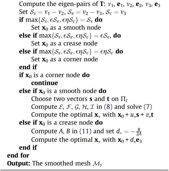
Algorithm 1 performs well for surface meshes without sharp features such as creases or corners. In reality, however, sharp features are commonly seen and crucial in precisely representing geometric features of a mesh. To this end, we classify the surface nodes into three categories: (1) smooth nodes with low curvature in the neighborhood, (2) crease nodes with low curvature in one direction and high curvature in another (typically perpendicular to the first direction), and (3) corner nodes, where at least three creases intersect. We define crease and corner nodes as feature nodes and impose some special restrictions on them during the mesh smoothing process. Specifically, a crease node moves only along the direction of the crease and a corner node remains unchanged.

Algorithm 1.

Suboptimal Delaunay triangulation (S-ODT)

Motivated by [33,22], we distinguish between smooth and feature nodes by using the local structure tensor T at x₀ as defined below:

$$\mathbf{T}=\sum _{k=1}^N{\omega }_k{\mathbf{n}}_k{\mathbf{n}}_k^{\mathrm{T}}.$$ (9)

Here n_k is the unit normal vector of τ_k, calculated by 〈x₀, x_k, x_k+1〉. The weight ω_k is determined by $\frac{{\mathrm{S}}_k}{{\mathrm{S}}_{\max }}\exp (-g_k∕\sigma )$, where S_k is the area of τ_k, S_max = max_i=1,…NS_i,g_k is the distance from x₀ to the barycenter of τ_k, and σ is the average edge length of the surface mesh.

Note that T is a semi-positive definite symmetric matrix and has three real eigenvalues. We decompose T using the eigen-analysis method and decide the type of x₀ based on the distribution of the eigenvalues of T. Let v₁≥ v₂≥ v₃ be the eigenvalues of T and e₁, e₂ and e₃ be the corresponding eigenvectors. Let ${\mathcal{S}}_s={\mathcal{V}}_1-{\mathcal{V}}_2$, ${\mathcal{S}}_e={\mathcal{V}}_2-{\mathcal{V}}_3$ and ${\mathcal{S}}_c={\mathcal{V}}_3$, the type of is x₀ following scheme:

$$\max \{{\mathcal{S}}_s,∊{\mathcal{S}}_e,∊\eta {\mathcal{S}}_c\}=\{\begin{array}{cc}{\mathcal{S}}_c:\hfill & {\mathbf{x}}_0\text{is a smooth node},\hfill \\ ∊{\mathcal{S}}_e:\hfill & {\mathbf{x}}_0\text{lies on a crease curve with direction}{\mathbf{e}}_3\hfill \\ ∊\eta {\mathcal{S}}_c:\hfill & {\mathbf{x}}_0\text{is a corner node}.\hfill \end{array}\phantom{\}}$$ (10)

Here, the sensitivity parameters ε and η are both set to be 2 according to [33].

In the mesh smoothing process, Algorithm 1 is still applicable when x₀ is a smooth node. When x₀ is a corner node, we just keep it unchanged. When x₀ is a crease node, however, we move x₀ to the optimal position by solving (5) along the direction of the crease. Therefore, we assume x′ = x₀ + de₃ and compute the optimal value d_* by minimizing (5) along e₃. The computation of d_* is similar to that of u_*, v_* in Algorithm 1. First, we compute the corresponding coefficients in the following way:

$$\{\begin{array}{c}A=C+\sum _{k=1}^n\left[{\mathbf{e}}_3\right({\mathbf{X}}_k+{\mathbf{X}}_{k+1}\left)\det \right({\mathbf{e}}_3,{\mathbf{X}}_{k+1}-{\mathbf{X}}_k,\mathbf{n}\left)\right],\hfill \\ B=\sum _{k=1}^N\left[{\mathbf{e}}_3\right({\mathbf{X}}_k+{\mathbf{X}}_{k+1}\left)\det \right({\mathbf{X}}_k,{\mathbf{X}}_{k+1},\mathbf{n})+({\mathbf{X}}_k^2-{\mathbf{X}}_k{\mathbf{X}}_{k+1}+{\mathbf{X}}_{k+1}^2\left)\det \right({\mathbf{e}}_3,{\mathbf{X}}_{k+1}-{\mathbf{X}}_k,\mathbf{n}\left)\right].\hfill \end{array}\phantom{\}}$$ (11)

Then the scalar d_* is computed by $d_{\ast }=-\frac{B}{2A}$. The process is summarized in Algorithm 2.

Algorithm 2.

Feature-preserving S-ODT

2.5. Feature-preserving, noise-removing mesh quality improvement

Our method can be readily adapted to remove mesh noise while improving mesh quality and still retaining the feature-preserving property. In the basic S-ODT algorithm (Algorithm 1), the optimal position is assumed to be on the tangent plane at x₀ of the surface mesh. When there is noise on the surface mesh, a common strategy is to fit a plane (or higher order polynomials) to the neighboring nodes of each vertex and project the vertex onto the plane [28]. Sharp features may be preserved by considering anisotropic local neighborhoods [35]. In our current work, we utilize a weighted least squares fitting strategy as detailed below [39].

As described in Section 2.4, each mesh node can be classified into either a smooth node, a crease node or a corner node. We always keep the corner nodes unchanged. Suppose x₀ is a smooth node with neighboring nodes ${\left\{{\mathbf{x}}_k\right\}}_{k=1}^N$. The corresponding unit normal vectors at x₀ and its neighbors are ${\left\{{\mathbf{n}}_k\right\}}_{k=0}^N$. Then a plane can be fitted by solving the following weighted least squares problem:

$$\underset{x,n}{\min }\sum _{k=0}^N{w}_k{\left(\right({\mathbf{x}}_k-\stackrel{‒}{\mathbf{x}}\left)\stackrel{‒}{\mathbf{n}}\right)}^2,$$ (12)

where w_k is the weight of x_k, $\stackrel{‒}{\mathbf{x}}$ is a point on the fitting plane Π_f and $\stackrel{‒}{\mathbf{n}}$ is the unit normal vector of Π_f. The weights are set as follows:

$$w_0=1,w_k=L\left(r_k\right),\text{where}{r}_k={\mathbf{n}}_0\cdot {\mathbf{n}}_k,k=1,2,\dots ,N.$$

L(r) is a linear function on [cos(π/4),1] with L(cos(π/4)) = 0 and L(1) = 1.

The fitting plane Π_f can be computed by first determining $\stackrel{‒}{\mathbf{x}}$ and then $\stackrel{‒}{\mathbf{n}}$. Specifically, $\stackrel{‒}{\mathbf{x}}$ is the weighted average of x₀ and its neighbors:

$$\stackrel{‒}{\mathbf{x}}=\sum _{k=0}^N{W}_k{\mathbf{x}}_k∕\sum _{k=0}^N{W}_k.$$ (13)

$\stackrel{‒}{\mathbf{n}}$ is chosen to be the eigenvector corresponding to the smallest eigenvalue of the following matrix M [39]:

$$\mathbf{M}=\sum _{k=0}^N{W}_k({\mathbf{x}}_k-\stackrel{‒}{\mathbf{x}}){({\mathbf{x}}_k-\stackrel{‒}{\mathbf{x}})}^{\mathrm{T}}.$$

Simply projecting x₀ onto the fitting plane Π_f can suppress the mesh noise around x₀ but the mesh angle quality may not be improved and sometimes may become even worse. To achieve both mesh denoising and quality improvement, we replace the tangent plane Π_t in Algorithm 1 or Algorithm 2 with the fitting plane Π_f and accordingly replace x₀ with $\stackrel{‒}{\mathbf{x}}$ in the minimization of (5).

When x₀ is a crease node, a similar procedure is applied. The difference is that we fit a line instead of a plane by using some 2-ring neighboring nodes of x₀ and then project x₀ onto the fitted line. The neighboring nodes selected include x₀ itself, two neighbors along one direction of the crease line and two neighbors along the other direction of the crease line, where the crease line passing x₀ is defined as the crease direction determined by the tensor analysis procedure. The two neighbors along each direction are selected so that they are the closest to the crease line. The overall algorithm for feature-preserving mesh denoising and quality improvement is given in Algorithm 3.

Algorithm 3.

Feature-preserving & noise-removing S-ODT

3. Results and discussions

The presented algorithms have been tested on numerous surface meshes and we shall show some of the results below. We first apply the basic S-ODT algorithm (Algorithm 1) to several surface meshes without noise or sharp features. The bimba and elephant models are shown in Fig. 2a and Fig. 3a respectively. A closer look at the original bimba mesh and the angle histograms of these meshes are given in Fig. 2b and c and Fig. 3b and c. By applying Algorithm 1 to each mesh for 20 times, the mesh qualities are significantly improved, as can be seen from Fig. 2d–f and Fig. 3d–f.

Fig. 2.

The bimba mesh model. (a–c) Show the original surface mesh, a closer view and the angle histogram of the mesh. (d–f) Show the smoothed mesh and the corresponding histogram after applying the S-ODT (Algorithm 1) 20 times. The minimum and maximum angles in both meshes are indicated in red in the histograms. The original model is provided courtesy of IMATI and INRIA by the AIM@SHAPE Shape Repository. (For interpretation of the references to colour in this figure legend, the reader is referred to the web version of this article.)

Fig. 3.

The elephant mesh model. (a–c) Show the original surface mesh, a closer view and the angle histogram of the mesh. (d–f) Show the smoothed mesh and the corresponding histogram after applying the S-ODT (Algorithm 1) 20 times. The minimum and maximum angles in both meshes are indicated in red in the histograms. The model is provided courtesy of INRIA by the AIM@SHAPE Shape Repository. (For interpretation of the references to colour in this figure legend, the reader is referred to the web version of this article.)

In Fig. 4 we show how the minimum and maximum angles of the bimba and elephant models change with respect to the number of iterations by applying Algorithm 1. We can see that the mesh qualities are largely improved in the first five iterations, and further smoothing does not help much on mesh quality improvement. In order to measure the shape change between the original and smoothed meshes, we compute the symmetric Hausdorff distance between the meshes using the M.E.S.H. tool [40], and the results are illustrated in Fig. 5. The histograms in Fig. 5 show the absolute differences between the original and smoothed meshes. The maximal relative differences, defined as the ratio of the maximal absolute difference over the diagonal of the bounding box of a mesh, are 0.09% and 0.13% for the bimba and elephant models respectively.

Fig. 4.

The convergence of Algorithm 1. (a and b) Show how the minimal and maximal angles (in degrees) change with respect to the number of iterations applied to the bimba model. (c and d) Show how the minimal and maximal angles (in degrees) change with respect to the number of iterations applied to the elephant model.

Fig. 5.

The symmetric Hausdorff distance between the original and smoothed meshes. The distance is computed using the M.E.S.H. tool [40].

As mentioned in Section 2.2, the analytically-based S-ODT algorithm is a suboptimal solution to the ODT method on surfaces. Here we compare the S-ODT method with the numerical solution of the optimal problem (the ODT method on surfaces). The model we use is a triangular surface mesh of a biomedical molecule called RyR with 129 K vertices. Algorithm 1 is applied to this mesh for 20 times and it takes about 36 s. By contrast, a numerical method by using L-BFGS [41] is adopted to solve the original optimal problem in Eq. (3) and it takes about 2 min for five iterations, after which no significant improvement was observed. The resulting meshes as well as their qualities, however, are similar by using the two methods, as we can see from Fig. 6. A conclusion from this experiment is that the proposed S-ODT method can smooth a mesh as effectively as the numerically-based optimalization method but it takes much less time than the latter.

The feature-preserving S-ODT method (Algorithm 2) is tested on the noise-free fandisk model containing crease edges and corners. The algorithm is applied on the mesh for 20 times and the results are shown in Fig. 7a–f, where both angle histograms and curvature distributions before and after mesh smoothing are provided. Besides the significantly improved mesh quality, the sharp features are well preserved too. Note that the sensitivity parameters ε and η in Eq. (10) are both set to be 2 according to [33]. However, we believe that this value should be controlled by the user as the user is the best person to define the “noise” and “feature” in his/her data. Different parameter values would give different results of the node classification, which would produce different smoothing results as the three types of nodes (smooth, crease, and corner) are subject to different smoothing procedures in our algorithms. For example, larger sensitivity parameters would better preserve small “features” that may otherwise be treated as “noise” and smoothed out when small parameters are chosen. When both sensitivity parameter are small, almost all vertices are smooth nodes and no feature preservation can be achieved.

Fig. 7.

Illustration of the feature-preserving S-ODT method (Algorithm 2) and comparison with remeshing method in [18]. (a–c) Show the original noise-free fandisk model containing sharp edges and corners, its angle histogram, and the corresponding distribution map of mean curvatures. (d–f) Show the smoothed mesh with significantly improved angle quality and regularized curvatures. (g–i) Show the remeshing results using the method in [18]. The model is provided by the AIM@SHAPE Shape Repository.

The feature-preserving and noise-removing S-ODT method (Algorithm 3) is also applied for 20 times to three noisy meshes: the dragon head (Fig. 8), the Chinese lion (Fig. 9), and the noisy fandisk (Fig. 10). The mesh quality improvement is clearly demonstrated by the angle histograms in all these models and Fig. 11. The curvature distribution maps in Figs. 9 and 10 show high-performance mesh denoising effects. In addition, the noisy fandisk model (Fig. 10) confirms the feature-preserving property of our method. The bilateral filtering denoising technique is utilized and compared with our approach as shown in Fig. 10. In the figure, the mesh quality by the bilateral filtering is poor, and the curvature distribution is also worse than our method. It is worth pointing out that our method performs better than the bilateral filter because we pre-classify every vertex using the tensor analysis technique.

Fig. 8.

Mesh smoothing of the dragon head model. (a–c) Original mesh with noise and extremely low quality (mesh courtesy of Stanford University – 3D scanning repository). (d–f) Smoothed mesh with significantly improved quality. (g–i) Remeshed results using [17].

Fig. 9.

Illustration of the feature-preserving and noise-removing S-ODT method (Algorithm 3) and comparison with remeshing method in [18]. The original and smoothed meshes of the Chinese lion are shown on the top and middle respectively. The remeshed mesh is shown on the bottom. The model is provided courtesy of INRIA by the AIM@SHAPE Shape Repository.

Fig. 10.

Illustration of the feature-preserving and noise-removing S-ODT method (Algorithm 3). The original and smoothed meshes of the fandisk and their corresponding histograms and curvature maps are shown on the top and middle rows respectively. And the bilateral filtering [10] result is shown in the bottom row.

Fig. 11.

Illustration of the mesh quality improvement of S-ODT method (Algorithm 3) on the Venus and Angel models.

Tables 1 and 2 show quantitative comparisons between our S-ODT algorithms (with 20 iterations) and two other representative methods, Sun’s [35] and Ohtake’s [26], running on a Pentium IV PC of 2.0 GHz. Note that the dancer model (not shown due to space limit), also downloaded from the AIM@SHAPE Shape Repository, was included to fill the size gap of the other models shown in this paper. The mesh qualities after smoothing are provided in Table 1, where Sun’s method is excluded because it performs worse than Ohtake’s method on all the models considered. From Table 2 we can see that Sun’s method is fast but, like Ohtake’s, it lacks the ability of mesh quality improvement. While the running time of our method can be much reduced if only 5–10 iterations are applied, the biggest gain of our approach is the tremendously improved mesh quality. As shown in Fig. 12, the running time of the three variants of our algorithm are approximately linear to the number of vertices in the meshes.

Table 1.

Comparisons of min-angle improvement.

Models	Original	Ours	Ohtake’s
Dancer	0.8°	18.3° (Alg.1)	0.4°
Elephant	1.4°	17.9° (Alg.1)	0.2°
Bimba	1.4°	15.5° (Alg.1)	0.2°
RyR	4.9°	17.3° (Alg.1)	0.2°
Noise-free fandisk	0.0°	17.7° (Alg.2)	0.1°
Noisy fandisk	16.0°	18.4° (Alg.3)	0.4°
Chinese lion	0.2°	16.8° (Alg.3)	0.0°
Dragon head	0.3°	17.5° (Alg.3)	0.1°
Venus	1.0°	16.8° (Alg.3)	0.0°
Angel	0.1°	16.3° (Alg.3)	0.0°

Table 2.

Comparisons of running time (in seconds).

Models	Vertex number	Ours	Ohtake’s	Sun’s
Dancer	24,998	12.0 (Alg.1)	3.3	0.8
Elephant	52,099	16.6 (Alg.1)	7.6	1.0
Bimba	83,887	24.5 (Alg.1)	11.8	1.7
RyR	129,346	35.8 (Alg.1)	16.8	2.6
Noise-free fandisk	6475	4.5 (Alg.2)	2.0	0.1
Noisy fandisk	6475	6.3 (Alg.3)	3.0	0.1
Chinese lion	99,289	49.8 (Alg.3)	13.0	2.1
Dragon head	99,777	50.5 (Alg.3)	14.8	3.1
Venus	100,759	53.3 (Alg.3)	15.7	8.8
Angel	236,979	120.4 (Alg.3)	35.1	15.7

Fig. 12.

The running time of the three variants of our algorithm, measured on the models with mesh sizes shown in Table II.

Finally we would like to compare our S-ODT method with the surface remeshing technique [15-18], as both aim to generate meshes with high quality. There are two main differences between the two methods: (1) the S-ODT always keeps the connectivity between vertices in a mesh while the remeshing method does not because of the re-sampling on the mesh; (2) for a smooth, closed surface mesh, the S-ODT algorithm preserves exactly the volume of the original mesh while the remeshing method typically does not. In addition, we demonstrate in Table 3 some quantitative comparisons between our S-ODT method and several recent remeshing algorithms [16-18]. From the table we can see that the methods in [16] does not guarantee improvement of min angles. The method in [17] fails when the size of the input mesh is too large (e.g., RyR). In addition, the remeshed results by this method are not as smooth as ours, as shown in Fig. 8g–i. Although high-quality meshes generally can be achieved by using the method in [18] when the original meshes are noise-free and error-free, the quality is not guaranteed for noisy meshes. When the original mesh contains self-intersecting triangles (e.g., the noise-free fandisk model in Table 3), the method in [18] cannot fix the errors and often results in low-quality meshes. The two problems of [18] are further demonstrated in Fig. 7g–i and Fig. 9g–i respectively. Although our algorithms seem to perform better in dealing with self-intersections, there is no guarantee of mesh quality either. This is because self-intersections introduce inverted normal vectors to some triangles, which usually results in inaccurate estimation of tangent planes (see Eq. (4)). In some cases, our algorithms may fail in improving the minimal and maximal angles of some meshes (see Fig. 13 for example), where poorly-shaped triangles are formed by vertices mostly lying on sharp edges. In these cases, other methods such as remeshing [17] or vertex insertion/deletion may work better.

Table 3.

Comparisons of min-angle improvement between our method and remeshing techniques.

Model	Ours	Valette’s	Wang’s	Fuhrmann’s
Dancer	18.3° (Alg.1)	6.0°	20.9°	30.7°
Elephant	17.9° (Alg.1)	0.0°	14.9°	30.5°
Bimba	15.5° (Alg.1)	0.0°	21.55°	32.8°
RyR	17.3° (Alg.1)	0.2°	N/A	31.0°
Noise-free fandisk	17.7° (Alg.2)	0.0°	28.8°	0.0°
Noisy fandisk	18.4° (Alg.3)	0.0°	35.6°	34.0°
Chinese lion	16.8° (Alg.3)	0.0°	15.12°	4.23°
Dragon head	17.5° (Alg.3)	0.0°	33.11°	0.55°
Venus	16.8° (Alg.3)	0.0°	N/A	2.77°
Angel	16.3° (Alg.3)	0.0°	N/A	0.92°

Fig. 13.

An example for which our algorithm fails in improving the quality. (a) The original crank model, where poorly-shaped triangles are formed by vertices mostly lying on sharp edges. Note that all non-manifold vertices in the mesh have been removed by using the MeshLab tool (http://meshlab.sourceforge.net/) prior to applying our algorithm. (b–c) A closer view of the selected region and the angle histogram of the original mesh. (d–f) The processed mesh using our method (Algorithm 2) and the angle histogram. Overall, the sharp features are preserved and the histogram becomes more uniform after mesh smoothing. But the minimal and maximal angles are not improved. The original mesh is provided courtesy of INRIA by the AIM@SHAPE Shape Repository.

4. Conclusion

In this paper, we present a novel, analytical approach that shows excellent performance in simultaneously denoising a surface mesh, improving the mesh quality, and preserving sharp features. Although the proposed S-ODT method is a suboptimal solution to the original ODT formulation, it can generate comparable results to the latter one but with much less computational time. Our method has fast convergence: typically five iterations are sufficient to observe good mesh quality and smoothness. In addition, the symmetric Hausdorff distances show that the smoothed mesh undergoes little shape deformation from the original mesh.

Appendix A. From (2) to (3)

For any given x′, note that ${\tau }_k^{\prime }$ is the triangle formed by 〈x′, x_k, x_k+1〉. We compute

$${\int }_{x\in {\tau }_k^{\prime }}{f}_I(\mathbf{x}-{\mathbf{x}}^{\prime })-f(\mathbf{x}-{\mathbf{x}}^{\prime })\mathrm{d}\mathbf{x}.$$ (A.1)

By replacing x with x′ + λ₁(x_k − x′) + λ₂(x_k+1 − x′), where λ₁, λ₂ ≥ 0 and λ₁ + λ₂ ≤ 1. Let Y_k = x_k − x′ and Y_k+1 = x_k+1 − x′, we can rewrite f(x − x′) into the following form:

$$f(\mathbf{x}-\mathbf{x}\prime )={\lambda }_1^2{\mathbf{Y}}_k^2+2{\lambda }_1{\lambda }_2{\mathbf{Y}}_k{\mathbf{Y}}_{k+1}+{\lambda }_2^2{\mathbf{Y}}_{k+1}^2.$$ (A.2)

Note that f_I(x − x′) is the linear interpolation of f(x − x′) in ${\tau }_k^{\prime }$, f(x − x′) takes the following form:

$$\begin{array}{cc}\hfill f_I(\mathbf{x}-{\mathbf{x}}^{\prime })=& f\left(0\right)+{\lambda }_{1}f\left({\mathbf{Y}}_k\right)+{\lambda }_{2}f\left({\mathbf{Y}}_{k+1}\right)\hfill \\ \hfill & ={\lambda }_1{\mathbf{Y}}_k^2+{\lambda }_2{\mathbf{Y}}_{k+1}^2.\hfill \end{array}$$ (A.3)

By substituting (A.2) and (A.3) for f(x − x′) and f_I(x − x′) respectively in (A.1), we have

$$\begin{array}{cc}\hfill & {\int }_{x\in {\tau }_k^{\prime }}{f}_I(\mathbf{x}-{\mathbf{x}}^{\prime })-f(\mathbf{x}-{\mathbf{x}}^{\prime })\mathrm{d}\mathbf{x}\hfill \\ \hfill =& {\int }_0^1\mathrm{d}{\lambda }_1{\int }_0^{1-{\lambda }_1}\left[\right({\lambda }_1-{\lambda }_1^2){\mathbf{Y}}_k^2+({\lambda }_2-{\lambda }_2^2){\mathbf{Y}}_{k+1}^2-2{\lambda }_1{\lambda }_2{\mathbf{Y}}_k{\mathbf{Y}}_{k+1}\mathrm{d}{\lambda }_2]\mid \mid {\mathbf{Y}}_k\times {\mathbf{Y}}_{k+1}\mid \mid \hfill \\ \hfill =& \frac{1}{12}({\mathbf{x}}_k^2+{\mathbf{x}}_{k+1}^2+{\mathbf{x}}^{\prime 2}-{\mathbf{x}}^{\prime }{\mathbf{x}}_k-{\mathbf{x}}^{\prime }{\mathbf{x}}_{k+1}-{\mathbf{x}}_k{\mathbf{x}}_{k+1}){\mathcal{S}}_k^{\prime }\hfill \\ \hfill =& \frac{1}{24}[{({\mathbf{x}}_k-{\mathbf{x}}^{\prime })}^2+{({\mathbf{x}}_{k+1}-{\mathbf{x}}^{\prime })}^2+{({\mathbf{x}}_{k+1}-{\mathbf{x}}_k)}^2]{\mathcal{S}}_k^{\prime },\hfill \end{array}$$ (A.4)

where ${\mathrm{S}}_k^{\prime }=\mid \mid {\mathbf{Y}}_k\times {\mathbf{Y}}_{K+1}\mid \mid ∕2$ is the area of ${\tau }_k^{\prime }$ and depends on the current vertex x′.

By dropping the constant that does not affect the optimal solution, we can rewrite the error function in (2) as follows:

$$E\left({\mathbf{x}}^{\prime }\right)=\sum _{k=1}^N[{({\mathbf{x}}_k-{\mathbf{x}}^{\prime })}^2+{({\mathbf{x}}_{k+1}-{\mathbf{x}}^{\prime })}^2+{({\mathbf{x}}_{k+1}-{\mathbf{x}}_k)}^2]{\mathcal{S}}_k^{\prime }.$$

Appendix B. Proof of ${\Sigma }_{k=1}^N{\mathrm{D}}_k^{\prime }\equiv C$

The determinant ${\mathrm{D}}_k^{\prime }$ in (5) has another form:

$${\mathrm{D}}_k^{\prime }=\det ({\mathbf{x}}_k-{\mathbf{x}}^{\prime },{\mathbf{x}}_{k+1}-{\mathbf{x}}^{\prime },\mathbf{n})=\left[\right({\mathbf{x}}_k-{\mathbf{x}}^{\prime })\times ({\mathbf{x}}_{k+1}-{\mathbf{x}}^{\prime }\left)\right]\mathbf{n}.$$

Thus we have

$$\begin{array}{cc}\hfill \sum _{k=1}^N{\mathrm{D}}_k^{\prime }=& \sum _{k=1}^N\left[\right({\mathbf{x}}_k-{\mathbf{x}}^{\prime })\times ({\mathbf{x}}_{k+1}-{\mathbf{x}}^{\prime }\left)\right]\mathbf{n}\hfill \\ \hfill =& \sum _{k=1}^N\left[\right({\mathbf{x}}_k\times {\mathbf{x}}_{k+1})+({\mathbf{x}}_{k+1}-{\mathbf{x}}_k)\times {\mathbf{x}}^{\prime }]\mathbf{n}\hfill \\ \hfill =& \mathbf{n}\sum _{k=1}^N({\mathbf{x}}_k\times {\mathbf{x}}_{k+1})+\mathbf{n}\left[\sum _{k=1}^N({\mathbf{x}}_{k+1}-{\mathbf{x}}_k)\times {\mathbf{x}}^{\prime }\right].\hfill \end{array}$$

Note that ${\Sigma }_{k=1}^N({\mathbf{x}}_{k+1}-{\mathbf{x}}_k)=0$, thus the sum of all ${\mathrm{D}}_k^{\prime }$ is a constant.

Appendix C. Computing the coefficients in (8)

Note that x′ = x₀ + us + vt, the objective function in (5) is equivalent to:

$$\begin{array}{cc}\hfill \stackrel{‒}{E}\left({\mathbf{x}}^{\prime }\right)=& \sum _{k=1}^N[{({\mathbf{x}}_k-{\mathbf{x}}^{\prime })}^2+{({\mathbf{x}}_{k+1}-{\mathbf{x}}^{\prime })}^2+{({\mathbf{x}}_{k+1}-{\mathbf{x}}_k)}^2]{\mathrm{D}}_k^{\prime }\hfill \\ \hfill =& \sum _{k=1}^N[{({\mathbf{X}}_k-{\mathbf{X}}^{\prime })}^2+{({\mathbf{X}}_{k+1}-{\mathbf{X}}^{\prime })}^2+{({\mathbf{X}}_{k+1}-{\mathbf{X}}_k)}^2]{\mathcal{D}}_k^{\prime },\hfill \end{array}$$

where X_i = x_i − x₀, X′= x′ − x₀ = us + vt and ${\mathcal{D}}_k^{\prime }={\mathrm{D}}_k^{\prime }=\det ({\mathbf{X}}_k-{\mathbf{X}}^{\prime },{\mathbf{X}}_{k+1}-{\mathbf{X}}_k,\mathbf{n})=\det ({\mathbf{X}}_k,{\mathbf{X}}_{k+1},\mathbf{n})-\det ({\mathbf{X}}^{\prime },{\mathbf{X}}_{k+1}-{\mathbf{X}}_k,\mathbf{n})$. Let ${\mathcal{S}}_k$ denote ${\mathbf{X}}_k^2-{\mathbf{X}}_k{\mathbf{X}}_{k+1}+{\mathbf{X}}_{k+1}^2$, we have:

$$\begin{array}{cc}\hfill \stackrel{‒}{E}\left({\mathbf{x}}^{\prime }\right)=& 2\sum _{k=1}^N[{\mathbf{X}}^{\prime 2}-({\mathbf{X}}_k+{\mathbf{X}}_{k+1}){\mathbf{X}}^{\prime }+({\mathbf{X}}_k^2-{\mathbf{X}}_k{\mathbf{X}}_{k+1}+{\mathbf{X}}_{k+1}^2\left)\right]{\mathcal{D}}_k^{\prime }\hfill \\ \hfill =& 2\left\{C{\mathrm{X}}^{\prime 2}-\sum _{k=1}^N\left[\right({\mathbf{X}}_k+{\mathbf{X}}_{k+1}){\mathbf{X}}^{\prime }{\mathcal{D}}_k^{\prime }+{\mathcal{S}}_k{\mathcal{D}}_k^{\prime }]\right\}\hfill \\ \hfill =& 2\{C(u^2+v^2)-(u\mathbf{s}+v\mathbf{t})\sum _{k=1}^N({\mathbf{X}}_k+{\mathbf{X}}_{k+1})\phantom{\}}\hfill \\ \hfill & \times \det ({\mathbf{X}}_k,{\mathbf{X}}_{k+1},\mathbf{n})+(u\mathbf{s}+v\mathbf{t})\sum _{k=1}^N({\mathbf{X}}_k+{\mathbf{X}}_{k+1})\hfill \\ \hfill & \times \det (u\mathbf{s}+v\mathbf{t},{\mathbf{X}}_{k+1}-{\mathbf{X}}_k,n)+\sum _{k=1}^N{\mathcal{S}}_k\left[\det \right({\mathbf{X}}_k,{\mathbf{X}}_{k+1},\mathbf{n})-\det (u\mathbf{s}+v\mathbf{t},{\mathbf{X}}_{k+1}-{\mathbf{X}}_k,\mathbf{n}\left)\right]\}\hfill \\ \hfill & =2(\epsilon u^2+\mathcal{F}{v}^2+\mathcal{g}uv-\mathcal{H}u-\mathcal{I}v+\mathcal{J}),\hfill \end{array}$$ (C.1)

where $\epsilon ,\mathcal{F},\mathcal{G},\mathcal{H},\mathcal{I}$ take the same forms as in (8) and $\mathcal{J}={\Sigma }_{k=1}^N{\mathcal{S}}_k\det ({\mathbf{X}}_k,{\mathbf{X}}_{k+1},\mathbf{n})$.

Note that (C.1) is a quadratic function, it has a unique minimum if the Hessian matrix is positive definite:

$$\begin{array}{cc}\hfill & \epsilon >0,\hfill \\ \hfill & 4\epsilon \mathcal{F}>{\mathcal{G}}^2.\hfill \end{array}$$

In the implementation of our algorithms, these conditions were checked, but interestingly they were never violated on all the meshes we had tested.

Thus the optimal solution of (5) can be computed by solving the following linear system:

$$\left(\begin{array}{cc}\hfill 2\epsilon \hfill & \hfill \mathcal{G}\hfill \\ \hfill \mathcal{G}\hfill & \hfill 2\mathcal{F}\hfill \end{array}\right)\left(\begin{array}{c}\hfill u\hfill \\ \hfill v\hfill \end{array}\right)=\left(\begin{array}{c}\hfill \mathcal{H}\hfill \\ \hfill \mathcal{I}\hfill \end{array}\right).$$

Appendix D. Proof of the volume-preserving property

We shall prove that the constraint of moving the vertex x₀ on a specially-defined tangent plane can preserve the volume of a smooth, closed surface mesh. In our algorithms, the normal of the tangent plane at x₀ is defined as:

$$\mathbf{n}=\sum _{i=1}^N{\mathcal{S}}_i{n}_i,$$ (D.1)

where S_i and n_i are the area and unit normal vector of the incident triangle τ_i formed by {x₀, x_i, x_i+1}. Suppose all n_i’s point to the outside of the closed mesh.

In order to define a “local” volume around x₀ for the surface mesh, we need to have an “anchor” point y, which can be any point. For simplicity, we can choose y as the centroid of all the neighboring vertices of x₀. By connecting x₀ and y with all the neighboring vertices of x₀, we get a local, closed domain denoted by Ω. Using a similar idea, when x₀ moves to any new position x′ in the tangent plane defined by (D.1), the points x′, y and all neighboring vertices of x₀ form another local closed domain Ω′. We shall prove that |Ω| ≡ |Ω′| for any x′ in the tangent plane, where ∥ denotes volume of a closed domain. Note that both Ω and Ω′ can be divided into N tetrahedra. For example, the N tetrahedra forming Ω are {x₀, x₁, x₂, y}, {x₀, x₂, x₃, y}, …, {x₀, x_N, x₁, y}. Therefore, the volumes of Ω and Ω′ are the total volumes of the tetrahedra forming Ω and Ω′ respectively.

We now prove that the volume of Ω′ is independent of x′ (or equivalently |Ω′| ≡ |Ω|). For any tetrahedron σ_k in Ω′, the volume $\mid {\sigma }_k\mid =\frac{1}{3}{\mathrm{S}}_k\langle {\mathbf{n}}_k,{\mathbf{x}}^{\prime }-\mathbf{y}\rangle$. Thus, we have the following formula for the volume of Ω′:

$$\mid {\Omega }^{\prime }\mid =\sum _{k=1}^N\left(\frac{1}{3}{\mathcal{S}}_k\langle {\mathbf{n}}_k,{\mathbf{x}}^{\prime }-\mathbf{y}\rangle \right),$$ (D.2)

$$=\langle \frac{1}{3}\mathbf{n},{\mathbf{x}}^{\prime }-\mathbf{y}\rangle ,$$ (D.3)

$$\langle \frac{1}{3}\mathbf{n},{\mathbf{x}}^{\prime }-{\mathbf{x}}_0\rangle +\langle \frac{1}{3}\mathbf{n},{\mathbf{x}}_0-\mathbf{y}\rangle$$ (D.4)

Note that x′ is restricted in the tangent plane that passes through x₀ and takes n as the normal vector. Hence we have 〈n, x′ − x₀〉 ≡ 0. The volume becomes $\mid {\Omega }^{\prime }\mid =\langle \frac{1}{3}\mathbf{n},{\mathbf{x}}_0-\mathbf{y}\rangle$, which is independent of x′.

Please note that the above volume-preserving property does not apply to surface meshes with noise or sharp features. As described in Algorithm 2, we consider crease lines instead of tangent planes for sharp features. For surface meshes with noise (see Algorithm 3), tangent planes are approximated by using a fitting technique. The Eq. (D.1) does not apply to either case.

References

- [1].Chen L. Mesh smoothing schemes based on optimal Delaunay triangulations; 13th International Meshing Roundtable; 2004.pp. 109–120. [Google Scholar]
- [2].Desbrun M, Meyer M, Schröder P, Barr AH. SIGGRAPH 1999 Papers. New York, NY, USA; 1999. Implicit fairing of irregular meshes using diffusion and curvature flow; pp. 317–324. [Google Scholar]
- [3].Ohtake Y, Belyaev A, Seidel HP. Vision, Modeling, and Visualization 2002. Erlangen, Germany: 2002. Mesh smoothing by adaptive and anisotropic Gaussian filter applied to mesh normals; pp. 203–210. [Google Scholar]
- [4].Wang J, Yu Z. A novel method for surface mesh smoothing: applications in biomedical modeling; Proceedings of the 18th International Meshing Roundtable; 2009.pp. 195–210. [Google Scholar]
- [5].Nociar M, Ferko A. Feature-preserving mesh denoising via attenuated bilateral normal filtering and quadrics; Proceedings of the 26th Spring Conference on Computer Graphics; ACM, New York, NY, USA. 2010.pp. 149–156. [Google Scholar]
- [6].Bajaj CL, Xu G. Anisotropic diffusion of surfaces and functions on surfaces. ACM Transactions on Graphics. 2003;22:4–32. [Google Scholar]
- [7].Taubin G. A signal processing approach to fair surface design; Proceedings of the 22nd Annual Conference on Computer Graphics and Interactive Techniques; ACM, New York, NY, USA. 1995.pp. 351–358. [Google Scholar]
- [8].Choudhury P, Tumblin J. ACM SIGGRAPH 2005 Courses. ACM; New York, NY, USA: 2005. The trilateral filter for high contrast images and meshes; pp. 186–196. [Google Scholar]
- [9].Peng J, Strela V, Zorin D. A simple algorithm for surface denoising; Proceedings of the Conference on Visualization ’01; IEEE Computer Society, Washington, DC, USA. 2001.pp. 107–112. [Google Scholar]
- [10].Fleishman S, Drori I, Cohen-Or D. ACM SIGGRAPH 2003 Papers. ACM; New York, NY, USA: 2003. Bilateral mesh denoising; pp. 950–953. [Google Scholar]
- [11].Bade R, Haase J, Preim B. Simulation und Visualisierung. 2006. Comparison of fundamental mesh smoothing algorithms for medical surface models; pp. 289–304. 2006. [Google Scholar]
- [12].Zhang Y, Xu G, Bajaj C. Quality meshing of implicit solvation models of biomolecular structures. Computer Aided Geometric Design. 2006;23(6):510–530. doi: 10.1016/j.cagd.2006.01.008. [DOI] [PMC free article] [PubMed] [Google Scholar]
- [13].Yue W, Guo Q, Zhang J, Wang G. 3D triangular mesh optimization in geometry processing for CAD; Proceedings of the 2007 ACM Symposium on Solid and Physical Modeling; ACM, New York, NY, USA. 2007.pp. 23–33. [Google Scholar]
- [14].Mari J. a. F., Saito JH, Poli G, Zorzan MR, Levada ALM. Improving the neural meshes algorithm for 3D surface reconstruction with edge swap operations; Proceedings of the 2008 ACM Symposium on Applied Computing; ACM, New York, NY, USA. 2008.pp. 1236–1240. [Google Scholar]
- [15].Alliez P, Devillers O, Isenburg M. Isotropic surface remeshing; International Conference on Shape Modeling and Applications; 2003.pp. 49–58. [Google Scholar]
- [16].Valette S, Chassery JM, Prost R. Generic remeshing of 3D triangular meshes with metric-dependent discrete voronoi diagrams. IEEE Transactions on Visualization and Computer Graphics. 2008;14:369–381. doi: 10.1109/TVCG.2007.70430. [DOI] [PubMed] [Google Scholar]
- [17].Yan D-M, Lévy B, Liu Y, Sun F, Wang W. Isotropic remeshing with fast and exact computation of restricted voronoi diagram. Computer Graphics Forum. 2009;28(5):1445–1454. [Google Scholar]
- [18].Fuhrmann S, Ackermann J, Kalbe T, Goesele M. Direct resampling for isotropic surface remeshing, in: Proceedings of Vision; Modeling and Visualization 2010; Siegen, Germany. 2010.pp. 9–16. [Google Scholar]
- [19].Field D. Laplacian smoothing and Delaunay triangulations. Communications in Applied Numerical Methods. 1988;4(6):709–712. [Google Scholar]
- [20].Amenta N, Bern M, Eppstein D. Optimal point placement for mesh smoothing; Proceedings of the Eighth Annual ACM-SIAM Symposium on Discrete Algorithms; Philadelphia, PA, USA. 1997.pp. 528–537. [Google Scholar]
- [21].Zhou T, Shimada K. An angle-based approach to two-dimensional mesh smoothing; Proceedings, 9th International Meshing Roundtable; 2000.pp. 373–384. [Google Scholar]
- [22].Yu Z, Holst MJ, McCammon JA. High-fidelity geometric modeling for biomedical applications. Finite Elements in Analysis and Design. 2008;44(11):715–723. [Google Scholar]
- [23].Dyer R, Zhang H, Möler T. Delaunay mesh construction; Proceedings of the Fifth Eurographics Symposium on Geometry Processing, Eurographics Association; 2007.pp. 273–282. [Google Scholar]
- [24].Freitag LA. Trends in Unstructured Mesh Generation. 1997. On combining Laplacian and optimization-based mesh smoothing techniques; pp. 37–43. [Google Scholar]
- [25].Canann SA, Tristano JR, Staten ML. An approach to combined Laplacian and optimization-based smoothing for triangular, quadrilateral, and quad-dominant meshes; Proceedings of the 7th International Meshing Roundtable; 1998.pp. 479–494. [Google Scholar]
- [26].Ohtake Y, Belyaev AG, Bogaevski IA. Geometric Modeling and Processing 2000. IEEE; 2000. Polyhedral surface smoothing with simultaneous mesh regularization; pp. 229–237. [Google Scholar]
- [27].Nealen A, Igarashi T, Sorkine O, Alexa M. Laplacian mesh optimization; Proceedings of the 4th International Conference on Computer Graphics and Interactive Techniques in Australasia and Southeast Asia; ACM, New York, NY, USA. 2006.pp. 381–389. [Google Scholar]
- [28].Wang J, Yu Z. Quality mesh smoothing via local surface fitting and optimum projection. Graphical Models. 2011;73(4):127–139. doi: 10.1016/j.gmod.2011.01.002. [DOI] [PMC free article] [PubMed] [Google Scholar]
- [29].Chen L, Xu J. Optimal Delaunay triangulations. Journal of Computational Mathematics. 2004;22(2):299–308. [Google Scholar]
- [30].Chen L, Holst MJ. Efficient mesh optimization schemes based on optimal Delaunay triangulations. Computer Methods in Applied Mechanics and Engineering. 2011;200:967–984. [Google Scholar]
- [31].Alliez P, Cohen-Steiner D, Yvinec M, Desbrun M. Variational tetrahedral meshing. Proc. of 2005 ACM SIGGRAPH. 2005;24:617–625. [Google Scholar]
- [32].Tournois J, Wormser C, Alliez P, Desbrun M. Interleaving Delaunay refinement and optimization for practical isotropic tetrahedron mesh generation. ACM Transactions on Graphics. 2009;28:75:1–75:9. [Google Scholar]
- [33].Page DL, Sun Y, Koschan AF, Paik J, Abidi MA. Normal vector voting: crease detection and curvature estimation on large, noisy meshes. Graphical Models. 2002;64(3-4):199–229. [Google Scholar]
- [34].Jones TR, Durand F, Desbrun M. Non-iterative, feature-preserving mesh smoothing. ACM Transactions on Graphics. 2003;22:943–949. [Google Scholar]
- [35].Sun X, Rosin P, Martin R, Langbein F. Fast and effective feature-preserving mesh denoising. Transactions on Visualization and Computer Graphics. 2007;13(5):925–938. doi: 10.1109/TVCG.2007.1065. [DOI] [PubMed] [Google Scholar]
- [36].Vallet B, Lévy B. Spectral geometry processing with manifold harmonics. Computer Graphics Forum (Proceedings Eurographics) 2008;27:251–260. [Google Scholar]
- [37].Sun X, Rosin PL, Martin RR, Langbein FC. Random walks for feature-preserving mesh denoising. Computer Aided Geometric Design. 2008;25(7):437–456. [Google Scholar]
- [38].Li Z, Ma L, Jin X, Zheng Z. A new feature-preserving mesh-smoothing algorithm. The Visual Computer. 2009;25:139–148. [Google Scholar]
- [39].Ahn SJ. Least Squares Orthogonal Distance Fitting of Curves and Surfaces in Space. Springer; 2005. [Google Scholar]
- [40].Aspert N, Santa-Cruz D, Ebrahimi T. Mesh: measuring errors between surfaces using the hausdorff distance; Proceedings: 2002 IEEE International Conference on Multimedia and Expo, 2002 (ICME ’02); 2002.pp. 705–708. [Google Scholar]
- [41].Liu D, Nocedal J. On the limited memory bfgs method for large scale optimization. Mathematical Programming. 1989;45(1):503–528. [Google Scholar]