Stochastic multiplicative population growth predicts and interprets Taylor's power law of fluctuation scaling

Abstract

Taylor's law (TL) asserts that the variance of the density (individuals per area or volume) of a set of comparable populations is a power-law function of the mean density of those populations. Despite the empirical confirmation of TL in hundreds of species, there is little consensus about why TL is so widely observed and how its estimated parameters should be interpreted. Here, we report that the Lewontin–Cohen (henceforth LC) model of stochastic population dynamics, which has been widely discussed and applied, leads to a spatial TL in the limit of large time and provides an explicit, exact interpretation of its parameters. The exponent of TL exceeds 2 if and only if the LC model is supercritical (growing on average), equals 2 if and only if the LC model is deterministic, and is less than 2 if and only if the LC model is subcritical (declining on average). TL and the LC model describe the spatial variability and the temporal dynamics of populations of trees on long-term plots censused over 75 years at the Black Rock Forest, Cornwall, NY, USA.

1. Introduction

Understanding the spatial and temporal variability of natural and engineered living populations is a central challenge of ecology. Population fluctuations to low densities may increase risks of extinction, frustrating attempts at species conservation, and may cause genetic bottlenecks, which can have enduring evolutionary consequences. Fluctuations of fisheries, forests and agricultural crops have economic consequences and may directly affect human supplies of food, timber, fibre and fuel. High fluctuations of the densities of arthropod and molluscan vectors of human as well as animal diseases may increase risks of disease transmission. Hence it is important for scientific and practical reasons to understand the pattern and origins of fluctuations in population densities.

An important generalization about population variability is Taylor's law (TL). TL asserts that the variance of the density (individuals per area or volume) of a set of comparable populations is a power-law function of the mean density of those populations. TL is one of the most widely tested empirical patterns in ecology and is the subject of an estimated thousand papers [1,2]. It has been confirmed for hundreds of species or groups of related species in field observations [3–5] and laboratory experiments with stem cells [6] and ecological microcosms [7–9]. Numerous models have been proposed to explain TL under various assumptions [10–16] and probability distributions compatible with TL have been analysed [17–24]. Nevertheless, it remains unclear why the ecological pattern called TL is so widely observed, how its estimated parameters should be interpreted in terms of underlying population dynamics and when it should be expected to fail.

TL presupposes that the mean and variance of population density exist and are finite. TL asserts that

1.1

TL holds with b = 2 in populations with a constant coefficient of variation (CV) of population density, such as certain cell populations [2,6], because then the variance is proportional to (mean)².

TL has multiple forms, depending on how averaging is done in space and time. The most familiar forms of TL suppose that multiple spatially distinct populations (plots of trees, Petri dishes of bacteria) are censused at multiple points in time. The estimated population densities may be arranged in a rectangular table or matrix, with each row corresponding to one population and each column corresponding to one census date. If the mean and the variance over time of each population are calculated, as in Kaltz et al. [8], one examines a temporal form of TL by plotting the logarithm of the variance as a function of the logarithm of the mean, with one point per spatially distinct population (i.e. one point (log mean, log variance) per row of the data matrix). A spatial TL considers the same array of data but reverses the roles of space and time, as in Taylor et al. [24]. For each census (column of the matrix), the mean and the variance over distinct populations are computed, and then the log variance is plotted as a function of the log mean, with one point (log mean, log variance) per census (i.e. per column of the data matrix). Here, we empirically test a spatial TL for tree populations at the Black Rock Forest (BRF), Cornwall, NY, USA [25].

By exact mathematical calculations (see appendix A), not simulations, we proved that, under general conditions, the Lewontin–Cohen (LC) model [34] of stochastic population dynamics predicts a spatial TL in the limit of large time and provides an explicit, exact interpretation of its parameters. This means that, for spatially distinct populations with dynamics governed by the LC model, with identical parameters in every population, as time increases, the spatial mean and the spatial variance of populations within a census come increasingly close to a power-law pattern described by TL. The exponent of TL exceeds 2 if and only if the LC model is supercritical (growing on average), equals 2 if and only if the LC model is deterministic, and is less than 2 if and only if the LC model is subcritical (declining on average). We shall show that the LC model describes the temporal dynamics and TL describes the spatial variability of populations of trees in long-term plots censused over 75 years at BRF.

The LC model was first published in the same decade as Taylor's original report [3], has been widely discussed and applied [35–37], and until now has remained unconnected with TL. Our results show that, for large time, TL holds with parameters given by explicit, exact functions of population-dynamic parameters in the LC model when the assumptions of the LC model are valid. This connection links an ecological pattern (TL) with a population-dynamic model (LC) that can explain it.

2. Theoretical and empirical results

(a). Lewontin–Cohen model of stochastic multiplicative population growth

Suppose N(t) > 0 represents the density of a population at time t for each t = 0, 1, 2, … . The initial population density, N(0), may be a fixed positive number or a random variable that takes positive values with probability 1. Suppose A(t) represents the random factor by which population density grows or declines from time t to time t+1, so that

2.1

The LC model assumes that {A(t), t = 0, 1, 2,…} are independently and identically distributed (iid) and that each A(t) has finite mean M > 0 and finite variance V > 0, and finite CV(A(0)) = V^1/2/M > 0. Here, CV(A(0)) means the CV (s.d./mean) of A(0). When N(0) is a random variable, the LC model further assumes that N(0) is independent of all {A(t), t = 0, 1, 2,…}.

This model, sometimes called a geometric random walk (as opposed to the ordinary additive random walk), assumes that the combined effect of any demographic and environmental stochasticity is adequately represented by the multiplicative factor A(t), which is tantamount to ignoring demographic stochasticity at small population sizes. It assumes no density dependence of A(t) on N(t) at either low or high population densities (other possible assumptions are considered by Perry and co-workers [16,23,24]). It assumes no autocorrelations in A(t): knowing the value of A(t) gives no information about the distribution of any past or future A(t′).

This model and generalizations have been used for random breakage of rocks, the random accumulation of wealth and many other applications [38,39]. The assumption that A(t), t = 0, 1, 2,… are iid has recently been tested directly and confirmed in detail for fisheries stocks [40]. Here, it will be tested and confirmed for forest trees.

We always use log = log₁₀. The expectation is denoted by E(·). The spatial mean and the spatial variance of population density over spatially distinct replicates (independent realizations using identical parameters) at time t are, respectively, E(N(t)) and Var(N(t)) = E[(N(t))²] − [E(N(t))]². Define

2.2

and

2.3

Then, in the LC model, the limits in (2.2) and (2.3) exist and are independent of N(0) and, in the limit of large time, the mean and variance of population density at time t grow exponentially with increasing time t in proportion to μ^t and β^t (μ > 0, β > 0), respectively. For the LC model (appendix A, theorem A.1),

2.4

and

2.5

We now write TL (1.1) as Var(N(t)) = a(E(N(t)))^b. Taking logs of both sides yields a mathematical equivalent, the log-linear form of TL:

2.6

By definition, we say that TL applies to N(t) in the limit as t → ∞ if and only if there exist real constants a > 0 and b such that

2.7

We show (appendix A, theorem A.2) that if TL applies to N(t) exactly for all t (as defined in (2.6)) or in the limit as t → ∞ (as defined in (2.7)), then log β = blog μ, where b is the exponent in TL. If log μ ≠ 0, then

2.8

Because the numerator and the denominator on the right-hand side of (2.8) are independent of N(0), so is b. Moreover (appendix A, theorem A.3), if M ≠ 1, then the LC model implies that N(t) obeys TL in the limit as t → ∞ with

2.9

Equations (2.9) connect the initial population density N(0) and the mean M and variance V of A(t) with the coefficient a and exponent b of TL. When N(0) has zero variance (i.e. is a constant with probability 1), then the formula for a simplifies to a = (N(0))^{2 −b}. For the population density ratio defined as η(t) = N(t)/N(0), η(0) = 1 with probability 1 and η(t) obeys TL as t → ∞ with a = (1)^2−b = 1 and b given by (2.9) (appendix A, corollary to theorem A.3). These key formulae are sufficiently non-obvious to justify discussion.

First, how do the parameters of the LC model constrain the parameters of TL? From the mean M and variance V or CV(A(0)) of A(0), we can calculate b from the right-hand equation of (2.9), substitute that into the exponent in the denominator of the left-hand equation, and determine a from the mean and second moment of N(0). For any M such that 0 < M, M ≠ 1, we cannot have b = 2 if V > 0. Also, for any M such that 0 < M, M ≠ 1, if V = 0 (in that case the LC model is deterministic), then b = 2 and a = [CV(N(0))]² + 1 (from (2.9)). Ballantyne [41] pointed out a connection between deterministic models (V = 0) and TL exponent b = 2.

On the other hand, for a fixed V > 0, we have 0 < M < 1 (population density decreases on average) if and only if b < 2. In particular, b = 1 (the population variance depends linearly on the population mean) if and only if V = M−M², and b = 0 (the population variance is independent of the population mean) if and only if V = 1−M², and b decreases from an upper limit of 2 (as V ↓ 0) towards −∞ (as V ↑ ∞). For a fixed V > 0, b > 2 if and only if M > 1, when the LC model is supercritical (population density increases on average). For a fixed M > 1, the bigger V is, the bigger b is.

Conversely, how do the parameters of TL constrain the parameters of the LC model? When b ≠ 2 and N(0) is a positive constant,

2.10

However, a and b are not sufficient to calculate separately the values of the mean M and the variance V of A(t) because they are confounded in the right-hand side of (2.9). But given b and M > 0, M ≠ 1, we find

2.11

Thus b and M are not each free to vary independently of the other: when M ≠ 1, then (CV(A(0)))² > 0 if and only if (b−2)logM > 0, and (CV(A(0)))² = 0 if and only if (b−2) logM = 0.

A transparent example, not intended to be biologically realistic, is informative on a significant point of theory. Suppose A(0) = d₁ = 7/10 with probability 1/2, and A(0) = d₂ = 6/5 with probability 1/2, and all A(t) are iid copies of A(0), as the LC model assumes. Then, from (2.9)

But 0 < b < 1 is impossible for exponential dispersion models and Tweedie distributions ([19, p. 133, theorem 2]; [42, p. 130, table 4.1]). Hence, this example demonstrates that exponential dispersion models and Tweedie distributions do not include all distributions that obey TL in the limit of large t. A comprehensive statistical theory of TL will have to go beyond exponential dispersion models and Tweedie distributions.

(b) Empirical example from Black Rock Forest

These theoretical analyses calculated, for each time t, the spatial mean E(η(t)) of the population density ratio η(t) = N(t)/N(0) and the spatial variance Var(η(t)) of the population density ratio, averaging over spatially distinct replicates (or ‘realizations’ in probability theory) of the LC population process at a given time, not averaging over time. The analyses demonstrated that as t gets larger, logVar(η(t))−b log E(η(t)) approaches log a = log 1 = 0.

Testing this theory using data from six long-term study plots in BRF [25], Cornwall, NY, required three steps. We give the data in the electronic supplementary material.

Step 1 used time-series of censuses of the trees to test whether the LC model described the temporal dynamics of tree population density by plot. Were the changes in population density independently and identically distributed over time and plots? Yes. So it was meaningful to calculate the mean M and the variance V of the changes A(p,t) = N(p,t+1)/N(p,t) pooled from all six plots, labelled p = 1, … , 6, at all census dates t except for the last census.

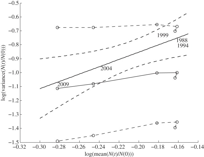
Step 2 interpreted six plots as spatially distinct replicates of the LC model. With this empirical interpretation, we tested whether the spatial variation of the population density ratio of trees η(t) among the six plots, calculated at each of the five most recent censuses (1988, 1994, 1999, 2004 and 2009), was described by the spatial TL. Was the logarithm of the variance (over six plots in each census) of the population density ratio η(t) linearly related to the logarithm of the mean (over six plots in each census) of the same population density ratio? Yes. So a spatial TL held.

As step 1 was approximately consistent with the LC model, and as step 2 was approximately consistent with a spatial TL, step 3 tested whether the slope b of the spatial log-linear TL in step 2 was consistent with the slope predicted from the LC model in step 1 (see appendix A) and whether the LC model in finite time could predict the observed variance. Did the LC model and the spatial TL fit together as theory predicted? Yes.

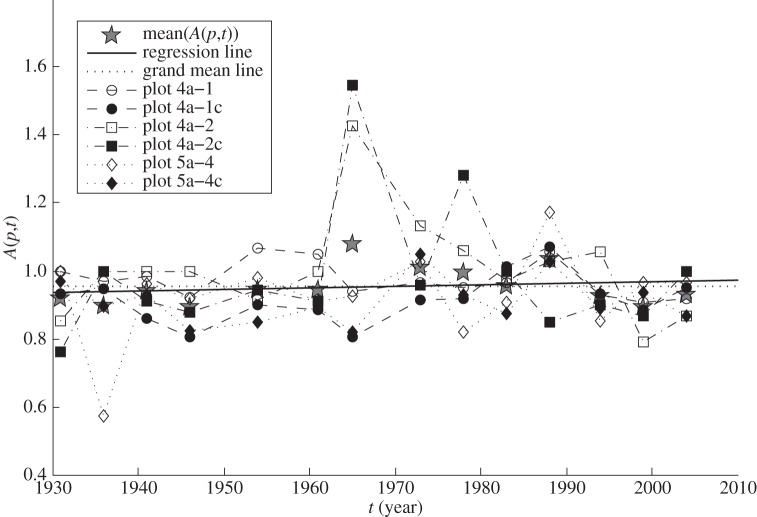
We give the details of the statistical analysis in appendix A and summarize here. In each of six long-term plots, the number of trees with diameter at breast height ≥ 1 inch (2.54 cm) was counted 15 times in the calendar years t = 1931, 1936, 1941, … , 2009 at intervals of nearly 5 years. For each plot p and each census year t, the density of trees N(p,t) was calculated as the number of trees divided by the corresponding area of plot p, and the ratio of successive population densities A(p,t) = N(p,t + δt)/N(p,t) was calculated using a nearly 5-year time step δt from the data of 1931 through to 2009. Figure 1 shows the six time-series of A(p,t), one time-series for each plot p. For each plot p separately, the first-, second- and third-order autocorrelations of the time-series of 14 values of A(p,t) were not statistically significant at the 0.05 level. Statistical tests failed (with one exception) to reject the null hypotheses that A(p,t) were independently and identically distributed (appendix A). Hence, the LC model described acceptably the temporal dynamics of tree population density in these data. Figure 2 shows the frequency histogram of the 84 (=6 plots × 14 intervals of time) values of A(p,t) when A(p,t) from all plots were pooled. Estimating M and V (appendix A and table 1), the key parameters of the LC model, completed step 1.

Figure 1.

Time-series of the ratio of the density of trees in a census year to the density of trees in each preceding census year approximately 5 years earlier, shown as a function of the earlier year. Solid markers indicate control plots. Open markers indicate plots thinned in 1930 before long-term observations began. The year-specific spatial means (grey stars) of E_p(A(p,t)) over six plots p were calculated at t = 1931, 1936, … , 2004, respectively. They differed little from the grand mean, 0.9535, the average of the 84 values of A(p,t) (dotted line). The least-squares regression line (solid line) fitted to all 84 values of A(p,t) as a function of t had a slope not significantly different from 0. Also, all six regression lines fitted to the 14 values of A(p,t) as a function of t for each plot p separately had slopes not significantly different from 0 (lines not shown). Thus, the average ratios did not change over years, by plot separately or pooled over plots.

Figure 2.

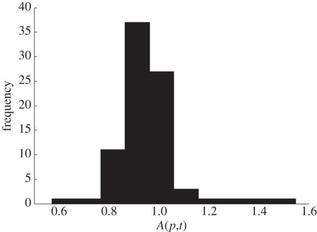
Frequency histogram of 84 values of A(p,t). The bootstrapped mean and variance of A(p,t), with the corresponding 95% CI, were recorded in appendix A, table 1.

Table 1.

Point and interval estimates of parameters in the Lewontin–Cohen model and a spatial Taylor's law. (For the Lewontin–Cohen model, parameter median values and 95% CIs from bootstrapping were recorded, because the distribution of each parameter was non-symmetrical. For the TL, b and log₁₀ a were estimated by fitting a straight line to the five data points, one point for each of the five most recent censuses (figure 3), using ordinary least squares. The CIs were generated from normal sampling theory rather than by bootstrapping. For the data points, nonlinearity was checked using least-squares quadratic regression on log–log coordinates. The coefficient of the squared term did not differ significantly from 0, so the null hypothesis of linearity was not rejected. When the median values of M and V were used in the formula for γ, γ = 1.6479, which fell within the bootstrapped 95% CI.)

model	parameter	point estimate	2.5% percentile	97.5% percentile
LC	M (mean of A(p,t))	0.9534	0.9280	0.9822
	V (variance of A(p,t))	0.0154	0.0069	0.0274
	γ (predicted slope)	1.6538	0.6641	1.8768
TL	b (least-squares slope)	2.6214	1.0728	4.1701
	log10 a (least-squares intercept)	−0.3289	−0.6579	0

In step 2, we tested whether a spatial TL described the spatial variability of the population density ratio in these long-term plots in BRF (figure 3).

Figure 3.

Log₁₀ variance of population density ratio in Black Rock Forest as a function of log₁₀ mean population density ratio from the five most recent censuses. The slope and intercept of the solid thick black line were estimated from the single linear regression using observed population density ratios in 1988, 1994, 1999, 2004 and 2009. Two thick dashed curves show the lower and upper 95% CIs for the fitted linear regression, indicating the region where the regression line would probably lie. The thin solid line connects open circles whose ordinates are the median estimates of the log variance from the LC model, log variance (t) = γ × log mean(t) + r(t), t = 11, 12, … , 15, from 10 000 bootstrapped samples of A(p,t), using formulae (A 11) and (A 12) for η(t) = N(t)/N(0). The upper and lower thin dashed lines connect open circles whose ordinates are respectively the 95% upper and lower bounds of the estimated log variance from the LC model based on the same bootstrap samples. For every census, the observed variance fell within the 95% CI predicted by the LC model. The 95% CI for log variance(t) = γ × log mean(t) without the adjustment for finite t included none of the observed values of log variance. See appendix A for details of methods and table 2 for numerical results.

In step 3, we compared the slope of the log-linear TL with the predicted slope from the LC model. The 95% confidence interval (CI) obtained from the LC model overlapped the corresponding 95% CI of the fitted log-linear TL (table 1). The 95% CI of the log variance predicted by the LC model contained the observed log variance from the data (figure 3 and table 2).

Table 2.

Point and interval estimates of log variance = γ × log mean + r(t) and log variance = γ × log mean where γ and r(t) are derived from the Lewontin–Cohen model ((A 11) and (A 12) respectively, see appendix A). (For every census, the 95% CI of log variance estimated from the LC model included the observed log variance when the term + r(t) was present and excluded the observed log variance when the term + r(t) was absent. Thus, the LC model could account for the observed log variance when, and only when, the correction + r(t) for finite time was included.)

year	observed log mean	observed log variance	log variance = γ × log mean + r(t)			log variance = γ × log mean
			median	2.5% percentile	97.5% percentile	median	2.5% percentile	97.5% percentile
1988	−0.1631	−0.7659	−1.0407	−1.3898	−0.7017	−0.2698	−0.3063	−0.1216
1994	−0.1611	−0.8041	−1.0032	−1.3500	−0.6682	−0.2665	−0.3026	−0.1201
1999	−0.1816	−0.7327	−1.0050	−1.3552	−0.6542	−0.3003	−0.3410	−0.1354
2004	−0.2458	−0.9661	−1.0817	−1.4457	−0.6723	−0.4066	−0.4617	−0.1833
2009	−0.2823	−1.0860	−1.1156	−1.4851	−0.6776	−0.4670	−0.5303	−0.2105

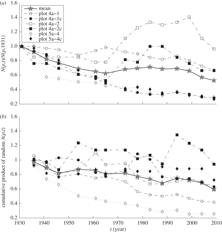
The theory developed above predicted that when the LC model leads to a spatial TL and when V > 0, the slope b will be less than 2 if and only if M < 1, that is, if and only if the average population declines over the long term. In BRF, the total number of trees in the six study plots declined from 551 in 1931 to 221 in 2009 and the density fell from 1718 to 689 stems per hectare. The trajectories from 1931 to 2009 of tree population density in each plot, divided by the population density in that plot in 1931, varied from plot to plot but had a generally declining trend (figure 4a). The median bootstrapped M was less than 1 and, as predicted, the median estimate of b from the LC model was less than 2 (table 1). Trajectories of relative population density simulated according to the assumptions of the LC model qualitatively resembled the observed trajectories (figure 4b). These trajectories were the cumulative products of A(p,t) sampled randomly, with replacement, from the observed values of A(p,t), regardless of plot or date. Thus the LC model qualitatively linked long-term decline or growth in population density with the slope of the spatial TL.

Figure 4.

Trajectories of tree population density, relative to population density in 1931 (a) of six long-term study plots in Black Rock Forest, and (b) of six illustrative simulations of the LC model. In both panels, grey stars showed the mean values at each time. (a) The observed relative tree population density N(p,t)/N(p,1931) for t = 1931, 1936, 1941, … , 2009, p = 1, … , 6. (b) The cumulative products of randomly selected values of the population growth factor A(p,t), namely A(p,t−5)A(p,t−10) ⋯ A(p,1931), for t = 1936, 1941, … , 2009, p = 1, … , 6. To form each cumulative product, each A(p,t) was sampled with replacement from the set of 84 observed values of A(p,t). The six lines in (b) illustrate six independent and identically distributed trajectories of the LC model.

3. Discussion and conclusion

The LC model provided a population-dynamical mechanism to explain a spatial TL in the limit of large time, according to an explicit mathematical calculation. Empirically, BRF data on the log variance and log mean of population density in the five most recent censuses were consistent with a spatial TL. BRF data on the changes in population density over 15 quinquennial censuses in six plots were consistent with the dynamic assumptions of the LC model. Using only the BRF data for the changes in population density and the observed mean population density, the LC model produced finite-time estimates of variance that were consistent with the observed variance in the five most recent censuses (figure 3 and table 2).

The LC model predicted log variance as a linear function of log mean plus a time-dependent residual term ((A 13) in appendix A). In the limit of large time, the size of this residual approached zero and the LC model gave a close approximation of the observed log variance. At finite time, the residual lowered the estimated log variance compared with the observed log variance. When plotted across different censuses, the log variance predicted by the LC model was a nonlinear function of the log mean. As time increased, the discrepancy between the log variance predicted by the LC model and the log variance observed or fitted by TL gradually diminished (figure 3).

Our analysis differed from many prior studies of TL in deriving TL from an existing, widely recognized model of population dynamics; in being exact, not a simulation; and in providing a detailed empirical test of the dynamic microstructure of the model in addition to the predicted TL. Prior models of TL covered a range of abstraction, from phenomenological to mechanistic [3–5,16,23,24,43–46]. Among the phenomenological models [13], some assumed a power–law relationship between the variance and mean [18,19,22,42] or imposed a constraint on the parameters of probability distributions that was equivalent to such an assumption [17]. Some phenomenological models [20,21] preceded Taylor's first paper [3] on the topic. By contrast, mechanistic models derived TL analytically or by simulation from models of ecological interactions or population dynamics [10–12,14,15,47–49]. The examples just given do not provide a complete review, nor does the much longer review by Eisler et al. [1], but they do suggest the diversity of approaches others have used, and how they have differed from ours.

The absence of statistically detectable autocorrelation in the six time-series of multiplicative increments A(p,t) may seem surprising but may have at least three simple explanations. First, the time between successive censuses is 5 years, more or less. Even if the factor of change in population density in a plot is autocorrelated from year y to the next year y+1, an exponential decay of autocorrelation with increasing lag δ between censuses in years y and y+δ and our finite sample sizes may reduce the 5-year autocorrelation, if it exists, to statistical insignificance. Second and third, for each plot, the autocorrelation in A(p,t) between year y and y+1 may be reduced by independent demographic stochasticity affecting the growth and death of trees, and by environmental stochasticity if the weather affecting the growth and survival of trees differs from year to year. The lack of autocorrelation in A(p,t) does not imply a lack of autocorrelation for N(p,t). Indeed, the first-order autocorrelation of time-series of N(p,t) is significant for each plot.

Further research is required to determine how plausible forms of density dependence would affect our conclusions and what happens when M = 1. Would Markovian dependence in the sequence {A(t)} of factors of change in population density lead to an asymptotic spatial TL? How would the parameters of a Markovian process be related to the parameters of TL? Can population-dynamical models lead to a temporal form of TL? TL is so widely observed in nature that improved understanding of its theoretical bases deserves priority.

Appendix A

(a). Lewontin–Cohen model

Theorem A.1. —

For the LC model, assume N(0) is a random variable that takes positive values with probability 1, has finite expectation 0 < E(N(0)) < ∞ and finite variance 0 ≤ Var(N(0)) < ∞, and is independent of {A(t), t = 0, 1, …}. Assume that {A(t), t = 0, 1, 2, …} are independently and identically distributed (iid) and that each A(t) has finite mean M = E(A(0)) > 0 and finite variance V = Var(A(0)) > 0. Then, the limits in (2.2) and (2.3) exist and

A1

and

A2

Proof. —

From (2.1), because A(t) are iid,

A3

Taking the log of both sides gives

A4

Dividing both sides by t and letting t → ∞ gives (2.4).

As N(0) and are independent, the variance of their product is [26, p. 709, eqn (2)]

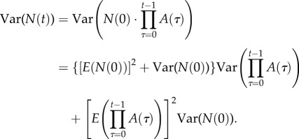
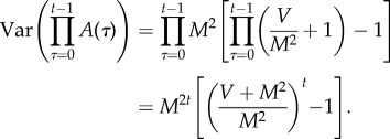
The variance of the product of iid variables A(τ), τ = 0,1, … ,t, is ([27, p. 218, eqn (4)]; [28, p. 55, eqn (1)])

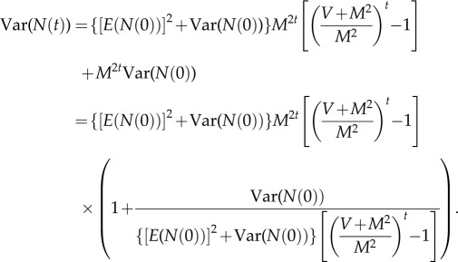
Hence

A5

Because V > 0 and M > 0 by assumption, (V + M²)M⁻² > 1. Hence, as t → ∞, the last factor on the right converges to 1 because the fraction converges to 0. Hence

A6

Also

so

A7

Therefore,

A8

hence

A9

This proves (2.5).□

(b). Taylor's law

Theorem A.2. —

If TL applies to N(t) exactly for all t or in the limit as t → ∞, then log β = b log μ. If log μ ≠ 0, then

A10

Proof. —

Divide log Var(N(t))−b log E(N(t)) by t and let t → ∞. Then, from (2.6) and (2.7) and the definitions of log μ (2.2) and log β (2.3), log β = 0+b log μ.□

Theorem A.3. —

Under the assumptions of theorem A.1, if M ≠ 1, (2.9) gives a unique pair of parameters such that N(t) obeys TL in the limit as t → ∞, as defined in (2.7), with these parameters.

Proof. —

Define

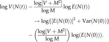
A11

Because M > 0, V > 0, M ≠ 1 by assumption, γ is well defined. Then, raising both sides of (A 3) to the power γ gives

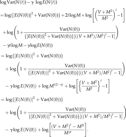
Subtracting γ logE(N(t)) from log Var(N(t)) gives

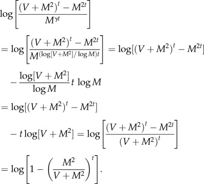
The definition of γ in (A 11) implies

Define

A12

Because M > 0 and V > 0, 0 < M²/(V + M²) < 1. As t → ∞, r(t) → 0, and

Therefore, the LC model implies that N(t) satisfies TL in the limit as t → ∞ with exponent b and coefficient a given by (2.9). Because TL holds, theorem A.2 implies that the exponent b of TL is uniquely specified by (A 11) or the right-hand equation in (2.9).□

For finite t, with these values of a and b, we have exactly, with the residual r(t) defined in (A 12),

A13

Corollary of theorem A.3. Under the assumptions of theorem A.3, the LC model implies TL for N(t)/N(0) in the limit as t → ∞, with coefficient a = 1 and exponent b given by (2.9).

Proof. —

Define η(t) = N(t)/N(0) for t = 0, 1, 2, … . Then η(0) = 1. Dividing both sides of (2) by N(0) yields

A14

This is exactly the same as (2.1) when N(0) = 1 with probability 1. The theorem implies that η(t) satisfies TL in the limit as t → ∞ with exponent b = log[V+M²]/logM and coefficient a = 1^2−b = 1.□

The initial density N(0) has no effect on b in the limit as t → ∞ because b measures the multiplicative factor by which variance of population density increases for a given multiplicative factor of increase in the mean population density. That multiplicative factor of increase does not depend on the starting population density. Consequently, uncertainty in N(0) may affect estimates of a but not estimates of b.

(c). Data analysis of Black Rock Forest long-term plots

The six long-term plots analysed here had areas from 0.038 to 0.089 ha with an average area 0.053 ha. The areas did not change over the years. Three plots were thinned prior to the first census in 1931, and three plots were undisturbed controls. From 1931 onwards, there were no further interventions. Trees were censused in, or (in a few cases) within one year of, the years 1931, 1936, 1941, 1946, 1954, 1961, 1965, 1973, 1978, 1983, 1988, 1994, 1999, 2004 and 2009. Most of the intervals between censuses were 5 years. The initial population densities in 1931 for the six plots were 922, 2351, 667, 1545, 2240 and 2412 stems per hectare, with mean 1690 and variance 583 617.

In step 1, testing the LC model, we assumed time-intervals were 5 years and used all censuses. The LC model assumed that A(p,t) were identically distributed over plots p and time t. To test this assumption over time, we compared the six values of A(p,t) = N(p,t + δt)/N(p,t), p = 1, … , 6, for each of the 14 censuses by one-way ANOVA by censuses, and found no significant differences at the 0.05 level of significance. To test whether each time-series A(p,t) were identical realizations for each of the six plots, we also compared the 14 values of A(p,t) = N(p,t+δt)/N(p,t), t = 1931, … , 2004, by one-way ANOVA among plots, the pooled three thinned plots with the pooled three control plots by one-way ANOVA between thinned and control, and the plots within treatments (thinned or control) by nested two-way ANOVA, and found no significant differences in the mean values at the 0.05 level of significance. ANCOVA showed no statistically significant difference in the slopes of regression lines fitted to the time-series of A(p,t) from different plots or treatments. The augmented Dickey–Fuller test gave no statistically significant evidence of non-stationarity. Four tests (O'Brien, Brown–Forsythe, Levene and Bartlett) were applied to test the homogeneity of variances of A(p,t) by treatments, plots and censuses. None of the tests rejected the hypothesis that the variance of A(p,t) in the pooled three thinned plots was identical to that in the pooled three control plots. The O'Brien, Brown–Forsythe and Levene tests did not reject the hypothesis that variances of A(p,t) over 14 censuses in each plot were identical. These tests did not reject the hypothesis that {A(t)} were identically distributed. However, the O'Brien, Levene and Bartlett tests rejected (p < 0.0001) the null hypothesis that the 14 variances over plots of A(p,t) for each of the 14 censuses were identical. The scatter of A(p,t) in 1965 (figure 1) was greater than the scatter before or after. This instance seemed to be an isolated, rather than a systematic, deviation from homogeneity of variances, and we did not correct our critical values for multiple simultaneous inference. We decided that the assumption of identical distributions was close enough to be a useful description of the data.

The LC model also assumed that {A(t)} were independently distributed. We tested this assumption in two ways. First, for the time-series of 14 values of A(p,t) of each plot p considered separately, the first-, second- and third-order autocorrelations were not statistically significant at the 0.05 level of significance. Second, for every pair of distinct years t₁, t₂, we computed the correlation between A(p,t₁) and A(p,t₂), p = 1, … , 6. Since we observed A(p,t) in 14 years, we had 14 × 13/2 = 91 pairwise correlations, of which seven (approx. 8%) were significant at the 5 per cent level of significance. The proportion of significant tests had 95% CI (0.0315, 0.1521), which is compatible with the null hypothesis that the significant tests occurred by chance alone. For every pair of different plots p₁ and p₂, 1 (approx. 7%) of 15 (= 6 × 5/2) correlations between A(p₁,t) and A(p₂,t), t = 1, … , 14 was significant at the 5 per cent level of significance, likewise giving no statistically significant evidence to reject the assumption that A(p,t) were independently distributed over time and plots.

Failing to reject the assumptions of the LC model, we estimated the mean M and the variance V of A(p,t) in each of 10 000 bootstrap samples (samples of each data point with equal probability and with replacement) of the 84 observed values of A(p,t) and recorded the median and 95% CIs. Then, from the M and V for each bootstrap sample, we calculated from (A 11) a value of γ, which is the LC model's prediction of the exponent b of TL, and recorded the median and 95% CI of the 10 000 bootstrapped values of γ (table 1).

In step 2, testing the spatial TL, we used the data from the five most recent censuses. In each selected census year (t = 1988, 1994, 1999, 2004, 2009), we calculated a spatial mean and a spatial variance of the population density ratio N(p,t)/N(p, 1931) over six plots. A single linear regression was fitted to the five pairs of log mean and log variance, pooled from each census, and the regression slope and intercept were estimated from normal theory (table 1).

TL was tested by applying linear regression to fit the log-linear form (2.6). We could also have fitted the power-law form (1.1) of TL by nonlinear least squares. However, tests of TL using other data from BRF [29] found no material differences between the results of these two modes of analysis, so we omitted here the analyses using nonlinear least squares.

Linear regression assumes no uncertainty in the abscissa of each data point [30]. But each study plot had uncertainty in the abscissa, log₁₀ mean population density (figure 3), because the mean was estimated from the population density ratio of six plots and was not known or controlled a priori. The same problem arose in fitting allometric power-laws of population density as a function of average body mass [31, pp. 153–154]. Neglecting uncertainty in the abscissa underestimates the true slope [2,30]. However, the use of linear regression was reasonable here because visual inspection showed that the fitted straight line approximated the data well (figure 3).

The bootstrap percentile method was applied to estimate the CIs of M, V and γ independently with 10 000 bootstrap samples used for each [32]. Computations of ANOVA, ANCOVA, homogeneity of variances, pairwise correlation, linear regression and quadratic regression were carried out using the JMP v. 9.0.2, analyze menu [33].

References

- 1.Eisler Z, Bartos I, Kertész J. 2008. Fluctuation scaling in complex systems: Taylor's law and beyond. Adv. Phys. 57, 89–142 10.1080/00018730801893043 (doi:10.1080/00018730801893043) [DOI] [Google Scholar]
- 2.Azevedo RBR, Leroi AM. 2001. A power law for cells. Proc. Natl Acad. Sci. USA 98, 5699–5704 10.1073/pnas.091485998 (doi:10.1073/pnas.091485998) [DOI] [PMC free article] [PubMed] [Google Scholar]
- 3.Taylor LR. 1961. Aggregation, variance and the mean. Nature 189, 732–735 10.1038/189732a0 (doi:10.1038/189732a0) [DOI] [Google Scholar]
- 4.Taylor LR, Woiwod IP. 1980. Temporal stability as a density-dependent species characteristic. J. Anim. Ecol. 49, 209–224 10.2307/4285 (doi:10.2307/4285) [DOI] [Google Scholar]
- 5.Taylor LR, Woiwod IP. 1982. Comparative synoptic dynamics. I. Relationships between inter- and intra-specific spatial and temporal variance/mean population parameters. J. Anim. Ecol. 51, 879–906 10.2307/4012 (doi:10.2307/4012) [DOI] [Google Scholar]
- 6.Klein AM, Simons BD. 2011. Universal patterns of stem cell fate in cycling adult tissues. Development 138, 3103–3111 10.1242/dev.060103 (doi:10.1242/dev.060103) [DOI] [PubMed] [Google Scholar]
- 7.Ramsayer J, Fellous S, Cohen JE, Hochberg ME. 2011. Taylor's law holds in experimental bacterial populations but competition does not influence the slope. Biol. Lett. 8, 316–319 10.1098/rsbl.2011.0895 (doi:10.1098/rsbl.2011.0895) [DOI] [PMC free article] [PubMed] [Google Scholar]
- 8.Kaltz O, Escobar-Paramo P, Hochberg M, Cohen JE. 2012. Bacterial microcosms obey Taylor's law: effects of abiotic and biotic stress and genetics on mean and variance of population density. Ecol. Process. 1, 5. 10.1186/2192-1709-1-5 (doi:10.1186/2192-1709-1-5) [DOI] [Google Scholar]
- 9.Hekstra DR, Leibler S. 2012. Contingency and statistical laws in replicate microbial closed ecosystems. Cell 149, 1164–1173 10.1016/j.cell.2012.03.040 (doi:10.1016/j.cell.2012.03.040) [DOI] [PubMed] [Google Scholar]
- 10.Kilpatrick AM, Ives AR. 2003. Species interactions can explain Taylor's power law for ecological time series. Nature 422, 65–68 10.1038/nature01471 (doi:10.1038/nature01471) [DOI] [PubMed] [Google Scholar]
- 11.Anderson RM, Gordon DM, Crawley MJ, Hassell MP. 1982. Variability in the abundance of animal and plant species. Nature 296, 245–248 10.1038/296245a0 (doi:10.1038/296245a0) [DOI] [Google Scholar]
- 12.Ballantyne F, IV, Kerkhoff AJ. 2007. The observed range for temporal mean-variance scaling exponents can be explained by reproductive correlation. Oikos 116, 174–180 10.1111/j.2006.0030-1299.15383.x (doi:10.1111/j.2006.0030-1299.15383.x) [DOI] [Google Scholar]
- 13.Engen S, Lande R, Saether B-E. 2008. A general model for analyzing Taylor's spatial scaling laws. Ecology 89, 2612–2622 10.1890/07-1529.1 (doi:10.1890/07-1529.1) [DOI] [PubMed] [Google Scholar]
- 14.Gillis DM, Kramer DL, Bell G. 1986. Taylor's power law as a consequence of Fretwell's ideal free distribution. J. Theor. Biol. 123, 281–287 10.1016/S0022-5193(86)80243-0 (doi:10.1016/S0022-5193(86)80243-0) [DOI] [Google Scholar]
- 15.Keeling MJ. 2000. Simple stochastic models and their power-law type behavior. Theor. Popul. Biol. 58, 21–31 10.1006/tpbi.2000.1475 (doi:10.1006/tpbi.2000.1475) [DOI] [PubMed] [Google Scholar]
- 16.Perry JN. 1988. Some models for spatial variability of animal species. Oikos 51, 124–130 10.2307/3565634 (doi:10.2307/3565634) [DOI] [Google Scholar]
- 17.Kemp AW. 1987. Families of discrete distributions satisfying Taylor's power law. Biometrics 43, 693–699 10.2307/2532005 (doi:10.2307/2532005) [DOI] [Google Scholar]
- 18.Kendal WS. 2004. Taylor's ecological power law as a consequence of scale invariant exponential dispersion models. Ecol. Complex. 1, 193–209 10.1016/j.ecocom.2004.05.001 (doi:10.1016/j.ecocom.2004.05.001) [DOI] [Google Scholar]
- 19.Jørgensen B. 1987. Exponential dispersion models. J. Royal Stat. Soc. B 49, 127–162 See http://www.jstor.org/stable/2345415. [Google Scholar]
- 20.Tweedie MCK. 1946. The regression of the sample variance on the sample mean. J. Lond. Math. Soc. 21, 22–28 10.1112/jlms/s1-21.1.22 (doi:10.1112/jlms/s1-21.1.22) [DOI] [Google Scholar]
- 21.Tweedie MCK. 1947. Functions of a statistical variate with given means, with special reference to Laplacian distributions. Proc. Cambridge Philos. Soc. 43, 41–49 10.1017/S0305004100023185 (doi:10.1017/S0305004100023185) [DOI] [Google Scholar]
- 22.Tweedie MCK. 1984. An index which distinguishes between some important exponential families. In Statistics: applications and new directions (eds Ghosh JK, Roy J.), pp. 579–604 Calcutta, India: Indian Statistical Institute [Google Scholar]
- 23.Perry JN, Taylor LR. 1985. Ades: new ecological families of species-specific frequency distributions that describe repeated spatial samples with an intrinsic power-law variance-mean property. J. Anim. Ecol. 54, 931–953 10.2307/4388 (doi:10.2307/4388) [DOI] [Google Scholar]
- 24.Taylor LR, Woiwod IP, Perry JN. 1978. The density-dependence of spatial behavior and the rarity of randomness. J. Anim. Ecol. 47, 383–406 See http://www.jstor.org/stable/3790 [Google Scholar]
- 25.Schuster WSF, Griffin KL, Roth H, Turnbull MH, Whitehead D, Tissue DT. 2008. Changes in composition, structure and aboveground biomass over seventy-six years (1930–2006) in the Black Rock Forest, Hudson Highlands, southeastern New York State. Tree Physiol. 28, 537–549 10.1093/treephys/28.4.537 (doi:10.1093/treephys/28.4.537) [DOI] [PubMed] [Google Scholar]
- 26.Goodman LA. 1960. On the exact variance of products. J. Am. Stat. Assoc. 55, 708–713 10.1080/01621459.1960.10483369 (doi:10.1080/01621459.1960.10483369) [DOI] [Google Scholar]
- 27.Shellard GD. 1952. Estimating the product of several random variables. J. Am. Stat. Assoc. 47, 216–221 10.1080/01621459.1952.10501165 (doi:10.1080/01621459.1952.10501165) [DOI] [Google Scholar]
- 28.Goodman LA. 1962. The variance of the product of K random variables. J. Am. Stat. Assoc. 57, 54–60 10.1080/01621459.1962.10482151 (doi:10.1080/01621459.1962.10482151) [DOI] [Google Scholar]
- 29.Cohen JE, Xu M, Schuster WSF. 2012. Allometric scaling of population variance with mean body size is predicted from Taylor's law and density-mass allometry. Proc. Natl Acad. Sci. USA 109, 15 829–15 834 10.1073/pnas.1212883109 (doi:10.1073/pnas.1212883109) [DOI] [PMC free article] [PubMed] [Google Scholar]
- 30.Snedecor GW, Cochran WG. 1980. Statistical methods, 7th edn Ames, IA: Iowa State University Press [Google Scholar]
- 31.Cohen JE, Carpenter SR. 2005. Species’ average body mass and numerical abundance in a community food web: statistical questions in estimating the relationship. In Dynamic food webs: multispecies assemblages, ecosystem development and environmental change (eds de Ruiter PC, Wolters V, Moore JC.), pp. 137–156 Amsterdam, The Netherlands: Elsevier [Google Scholar]
- 32.MathWorks Inc 2011. Matlab R2011b. Natick, MA: MathWorks Inc [Google Scholar]
- 33.SAS Institute Inc 2010. JMP 9.0.2. Cary, NC: SAS Institute Inc [Google Scholar]
- 34.Lewontin RC, Cohen D. 1969. On population growth in a randomly varying environment. Proc. Natl Acad. Sci. USA 62, 1056–1060 10.1073/pnas.62.4.1056 (doi:10.1073/pnas.62.4.1056) [DOI] [PMC free article] [PubMed] [Google Scholar]
- 35.Smith RH, Mead R. 1975. A note on population growth in a variable environment. Oecologia 20, 333–337 10.1007/BF00345523 (doi:10.1007/BF00345523) [DOI] [PubMed] [Google Scholar]
- 36.Williams BK, Nichols JD, Conroy MJ. 2002. Analysis and management of animal populations: modeling, estimation, and decision making. San Diego, CA: Academic Press [Google Scholar]
- 37.Drake JM. 2005. Population effects of increased climate variation. Proc. R. Soc. B 272, 1823–1827 10.1098/rspb.2005.3148 (doi:10.1098/rspb.2005.3148) [DOI] [PMC free article] [PubMed] [Google Scholar]
- 38.Aitchison J, Brown JAC. 1957. The lognormal distribution with special reference to its uses in economics. Cambridge, UK: Cambridge University Press [Google Scholar]
- 39.Johnson NL, Kotz S. 1970. Continuous univariate distributions 1, 2nd edn New York, NY: Wiley-Interscience [Google Scholar]
- 40.Niwa H-S. 2007. Random-walk dynamics of exploited fish populations. ICES J. Mar. Sci. 64, 496–502 10.1093/icesjms/fsm004 (doi:10.1093/icesjms/fsm004) [DOI] [Google Scholar]
- 41.Ballantyne F. 2005. The upper limit for the exponent of Taylor's power law is a consequence of deterministic population growth. Evol. Ecol. Res. 7, 1213–1220 [Google Scholar]
- 42.Jørgensen B. 1997. The theory of dispersion models. London, UK: Chapman & Hall [Google Scholar]
- 43.Taylor LR, Taylor RAJ. 1977. Aggregation, migration and population mechanics. Nature 265, 415–421 10.1038/265415a0 (doi:10.1038/265415a0) [DOI] [PubMed] [Google Scholar]
- 44.Taylor LR, Woiwod IP, Perry JN. 1980. Variance and the large scale spatial stability of aphids, moths and birds. J. Anim. Ecol. 49, 831–854 10.2307/4230 (doi:10.2307/4230) [DOI] [Google Scholar]
- 45.Taylor LR, Taylor RAJ, Woiwod IP, Perry JN. 1980. Behavioural dynamics. Nature 303, 801–804 10.1038/303801a0 (doi:10.1038/303801a0) [DOI] [Google Scholar]
- 46.Taylor LR. 1984. Assessing and interpreting the spatial distributions of insect populations. Annu. Rev. Entomol. 29, 321–357 10.1146/annurev.en.29.010184.001541 (doi:10.1146/annurev.en.29.010184.001541) [DOI] [Google Scholar]
- 47.Hanski I. 1980. Spatial patterns and movements in coprophagous beetles. Oikos 34, 293–310 10.2307/3544289 (doi:10.2307/3544289) [DOI] [Google Scholar]
- 48.Hanski I. 1987. Cross-correlation in population dynamics and the slope of spatial variance: mean regressions. Oikos 50, 148–151 10.2307/3565413 (doi:10.2307/3565413) [DOI] [Google Scholar]
- 49.Hanski I. 1982. On patterns of temporal and spatial variation in animal populations. Ann. Zool. Fennici 19, 21–37 [Google Scholar]