The Brain as a Complex System: Using Network Science as a Tool for Understanding the Brain

Abstract

Although graph theory has been around since the 18th century, the field of network science is more recent and continues to gain popularity, particularly in the field of neuroimaging. The field was propelled forward when Watts and Strogatz introduced their small-world network model, which described a network that provided regional specialization with efficient global information transfer. This model is appealing to the study of brain connectivity, as the brain can be viewed as a system with various interacting regions that produce complex behaviors. In practice, graph metrics such as clustering coefficient, path length, and efficiency measures are often used to characterize system properties. Centrality metrics such as degree, betweenness, closeness, and eigenvector centrality determine critical areas within the network. Community structure is also essential for understanding network organization and topology. Network science has led to a paradigm shift in the neuroscientific community, but it should be viewed as more than a simple “tool du jour.” To fully appreciate the utility of network science, a greater understanding of how network models apply to the brain is needed. An integrated appraisal of multiple network analyses should be performed to better understand network structure rather than focusing on univariate comparisons to find significant group differences; indeed, such comparisons, popular with traditional functional magnetic resonance imaging analyses, are arguably no longer relevant with graph-theory based approaches. These methods necessitate a philosophical shift toward complexity science. In this context, when correctly applied and interpreted, network scientific methods have a chance to revolutionize the understanding of brain function.

Introduction

Although graph theory has been around since the days of Euler, the field of network science is more recent and continues to gain popularity, particularly in the field of neuroimaging. The field was propelled forward when Watts and Strogatz (1998) introduced their small-world network model; this model described a network that provided regional specialization with efficient global information transfer. However, the concept of investigating phenomena at a systems level has been around since the middle of the 20th century. In the early days of psychology, Bavelas (1948) described two schools of thought that prevailed at the time; one group sought to break down people and situations into elements and attempted to explain behavior in terms of simple causal relationships. The other group attempted to explain behavior as a function of groups of factors constituting a dynamic whole. Although the aim of that particular study was to investigate communication, the idea of examining behavior at the group level introduced an important concept: the dynamic nature of a complex system cannot be understood by thinking of the system as comprised of independent elements. This concept also highlights the limits of reductionism; one cannot fully understand a complex system by only understanding its constituent parts (e.g., understanding the brain via knowledge about individual neurons). Rather, an approach is needed to utilize knowledge about the complex interactions within a system to understand the behavior of the system overall. With regards to the brain, the pertinent question to be asked is, “can a system like the brain be understood via knowledge about individual neurons (or voxels/sensors in the case of imaging), or is it best understood from information about how these neurons interact via structural or functional connections?” Complexity-driven methodologies provide powerful ways of understanding the dynamic interactions of different brain regions and how these interactions produce emergent behaviors.

Early applications of network science to the brain were performed in animal models (Jouve et al., 1998; Sporns et al., 2002, 2007) as well as humans (Rivière et al., 2002), and they focused on the structural topology of brain networks. Such an approach is appealing to the study of brain connectivity, as the brain can be viewed as a well-connected system comprised of various regions that interact with each other to produce complex behaviors. In practice, graph metrics such as clustering coefficient, path length, and efficiency measures are often used to characterize system properties at the local and global level. Moreover, centrality metrics such as degree, betweenness (Sporns et al., 2007), closeness (Sporns et al., 2007), eigenvector centrality (Lohmann et al., 2010), and leverage centrality (Joyce et al., 2010) have been used to identify critical areas in the network. In addition, detection of community structure has been essential for understanding the organization and topology of the network (Newman, 2006).

Greater use of these tools has led to a paradigm shift in the neuroscientific community. Nonetheless, network science should be viewed as more than a simple “tool du jour.” In order to fully appreciate the utility of network science within the neuroscience context, there needs to be a greater understanding of how network models apply to the brain; some metrics and models are appropriate for brain networks, whereas others are not. Further, less emphasis should be placed on univariate comparisons of these metrics to find significant group differences. Rather than ascribing significant differences or effects to particular voxels, as is historically done in functional neuroimaging, investigators should focus on understanding how the brain network as a whole is organized differently across various brains. This change in focus necessitates a philosophical shift in order to gain a greater understanding and appreciation of complexity in the brain. Without this shift, the network approaches to brain imaging risk becoming the next phrenology, following the path of traditional functional magnetic resonance imaging (fMRI) experiments over the past 20 years. When correctly applied and interpreted within the context of complexity science, network scientific methods have the chance to revolutionize our understanding of the functioning brain. In order to achieve this, a well-grounded understanding of complex systems analysis and how this applies to the brain is required. The goal of this article is not to provide a list of methods and metrics, as there are already extensive reviews on this topic (Bullmore and Sporns, 2009; Rubinov and Sporns, 2010). Rather, the goal of this article is to provide a more complexity-based framework for approaching brain networks with an emphasis on effectively using these tools to understand how the brain works.

Network Construction

Network science utilizes graph theory, which represents a system as a graph containing a set of objects, or nodes, connected by edges or links. From this graph, various analyses can be conducted to understand the topology and organization of the network. As shown in Figure 1, brain imaging data are first processed and analyzed to produce a matrix that denotes the strength of connection between nodes. For anatomical connectivity data, the connectivity matrix may represent the probability of fiber tracts between brain areas, whereas in functional connectivity data, the connectivity matrix may simply be the correlation matrix between time courses from different voxels/sensors. In functional connectivity data, it is common to apply a band-pass filter to regress out global signals and normalization parameters in order to reduce any confounds from physiological noise and subject motion (Fox et al., 2005). A threshold is then typically applied to this matrix to generate an adjacency matrix, after which network analyses ranging from simple graph metrics to community structure can be performed. When generating a network, there are several questions to consider: What are considered nodes in the network? What are considered links or connections in the network? Are strong and weak links differentiated (i.e., is there a threshold or is the network weighted)? Is there directedness in the network?

FIG. 1.

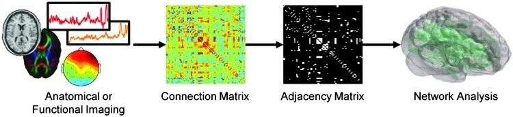
Network analysis schematic. Anatomical and functional brain imaging data are analyzed to produce a connection matrix, denoting the strength of connection between nodes. A threshold is commonly applied to the matrix to generate a binary adjacency matrix. From the adjacency matrix, various graph metric analyses can be performed.

Careful consideration is also needed with regard to the parcellation scheme chosen to construct the network. Depending on the parcellation scheme, the calculated metrics of the network can change (Wang et al., 2009). Further, comparison of networks can only be done when networks utilize the same parcellation scheme (Honey et al., 2007). Although many studies have used fixed region-based networks, voxel-based networks allow for investigation of intra-regional and inter-regional connectivity across brain regions (Eguíluz et al., 2005; van den Heuvel et al., 2008). In addition, a voxel-based network and a region-based network yield different degree distributions even if the networks are constructed from the same subject's fMRI data; as the network parcellation becomes more coarse, the degree distribution becomes more truncated, and high-degree nodes tend to be underrepresented (Hayasaka and Laurienti, 2010).

Network nodes and links

Ideally, a network model may consider each neuron as a node with every synapse functioning as a link. However, in practice, it is not possible to image or record from the estimated 10¹¹ (100 billion) neurons with an average 7000 synapses (Drachman, 2005), nor is it computationally feasible to analyze a network of that size. Even if such a model were feasible, then such a network would no longer be a model, but would represent an exact replica of the brain and would be no more comprehensible than the brain itself. Further, cognitive function is dependent on large-scale activation and coactivation of neuronal populations; thus, a model that integrates these populations is more useful (Sporns et al., 2005). Brain network analyses attempt to model the brain by selecting nodes based on regions from an atlas, such as the Automated Anatomical Labeling atlas (Tzourio-Mazoyer et al., 2002) or voxel-based networks (Eguíluz et al., 2005; van den Heuvel et al., 2008), where small blocks of tissue represent each node. It is anticipated that such models are effective, because the emergent properties can be evaluated in the absence of knowledge about each and every neuron.

Links between nodes in the network are dependent on the type of network being analyzed. Networks can be derived as anatomical or functional networks. Anatomical networks can be derived from histological samples or from diffusion tensor imaging (DTI) data. Some of the earliest work in anatomical brain networks was done in histological samples of the cat visual cortex (Sporns et al., 2007) and macaque cortex (Sporns et al., 2002). Connections in these networks were based on the physical connections that exist between brain regions. Anatomical networks can also be built from white matter tractography from DTI, with voxels of gray matter treated as nodes and the fiber tracts between brain regions as links (Hagmann et al., 2008). Although anatomical networks provide a good framework for showing what regions of the brain are directly connected, the brain exhibits functional coherence between seemingly distant brain regions. In fact, although some functional connectivity can be inferred from anatomical networks (Honey et al., 2007), the underlying structural connectivity alone does not determine functional connectivity, as two brain areas can be functionally connected without a direct anatomical connection between them (Honey et al., 2009). Networks based on functional connections can be employed to assess the consistent functional changes between different regions. Functional connections are typically based on magnitudes of temporal correlations. This can be assessed in fMRI (Eguíluz et al., 2005), electroencephalography (Micheloyannis et al., 2006; Stam et al., 2007), magnetoencephalography (Stam, 2004), and multielectrode array data (Srinivas et al., 2007).

A network can be represented as a matrix, with each row representing a node and each column on that row representing the relationship between the current node and every other node in the network. Links between nodes can be weighted or unweighted. Weighted links can represent size, density, or coherence of anatomical tracts in anatomical networks, whereas these links can represent strength of correlation or causal interactions in functional networks. In many network studies, unweighted (binary) networks are often used by applying a threshold and discretizing a weighted network; thus, links indicate the presence or absence of a connection. Although most studies in the literature use unweighted networks, weighted network analysis is being studied with greater interest. Studies using theoretical network models have evaluated weighted community structure (Kumpula et al., 2007), whereas weighted edges have been used to understand local clustering in trade and social networks (Saramäki et al., 2007). In the brain, weighted networks have been used to study network topology (Zamora-López et al., 2009) and modularity (Rubinov and Sporns, 2011). Weighted network analysis is likely to play a greater role in future brain network studies, as weighted edges provide more information about the relationship between node pairs. Although some studies advocate the use of fully connected weighted networks (Rubinov and Sporns, 2011), network threshold plays an important role in preserving certain topological properties. Without thresholding, weaker links representing spurious connections, noises, and indirect connections are left in the network, and such links can potentially create misleading results. Specifically, each node in the fully connected, weighted network has some direct interaction with every other node in the network. Information processing in such a system is no longer localized to clusters or neighborhoods but is shared globally. Nonetheless, weighted network analysis represents an area that is yet to be fully explored in the brain.

Network threshold

In functional networks, a threshold is often applied to the correlation matrix to remove links with very low strength. This process of thresholding often reduces the amount of data tremendously, thus leading to a sparse matrix comprised of strong connections, which represents only a fraction of all possible edges in the network. Without thresholding, all elements in the correlation matrix have to be considered as edges, thus resulting in a fully connected network. As just mentioned, analyzing such a network can become computationally burdensome, especially in larger-scale networks such as voxel-based functional connectivity networks. Thus, the choice of a threshold plays an important role in network construction, as it affects the density of connections and impacts network topology. Likewise, thresholding is important when comparing networks; a poor thresholding strategy can yield misleading results that artificially introduce significant differences or mask true differences in network topology (van Wijk et al., 2010).

Network thresholding approaches generally fall into three categories: fixed threshold, fixed average degree, and fixed edge density (van Wijk et al., 2010). A fixed threshold uses a single threshold based on one of three criteria: (1) using a 5% significance level in order to omit “spurious” links; (2) selecting an absolute threshold level across networks; or (3) selecting a threshold that keeps all nodes connected to the main component of the network. The drawback to this approach is that a single fixed threshold can generate networks that vary in connectivity and have different average degree across individuals or conditions (van Wijk et al., 2010). Another approach is to use fixed average degree, which ensures that all networks have the same average degree. Unlike the fixed threshold approach that uses the same correlation coefficient cut-off across networks, this method results in a different absolute threshold for each network. One problem that may arise is depending on the magnitude of the connectivity matrix values, the topology across networks may differ. To achieve the desired average degree, networks with generally weaker connectivity values (say average correlation coefficient R≈0.2) may include more weak links, whereas networks with higher connectivity values (say average R≈0.5) may omit strong links (van Wijk et al., 2010). Another option is to fix the edge density (or wiring cost: the proportion of the number of actual edges to the total possible number of edges) (Wang et al., 2009). This method is similar to fixing average degree, as degree (k) can be calculated by (N–1)d, where N is the number of nodes, and d is the edge density.

Network thresholding presents a difficult challenge, as there is no consensus on what strategy is best. Within the literature, it is common to show how graph metrics change over various thresholds (Achard et al., 2006; Stam, 2004; van den Heuvel et al., 2008; van Wijk et al., 2010). One possible solution is to select a threshold based on the size of the network. Laurienti and associates (2011) found a size-density relationship among self-organized networks that follows a power law. Assuming this relationship holds true, the size of the network may determine what threshold is best to achieve a desired edge density. Although most research focuses on the strong positive links in the network, there are newer models that incorporate strong negative (anticorrelated) links (Chen et al., 2011; Schwarz and McGonigle, 2011). Nonetheless, the choice of a threshold is still a point of debate within the field with some studies reporting results across the spectrum of a chosen thresholding approach. Alternatively, if one chooses to represent the network as a fully connected weighted network, then the issues associated with thresholding as just described are no longer a concern. However, as previously described, characterizing properties of a weighted network is still an area of ongoing research, and the best methods to employ for weighted network analyses are still unclear. Moreover, unlike a thresholded network that can be described by a sparse matrix, a fully connected weighted network includes a considerably large number of edges, and that may pose a serious computational challenge.

Information Flow in a Network

Before discussing the tools used to analyze brain networks, it is best to understand the concept of information flow, or traffic, in a network. Borgatti (2005) has written an excellent and thorough review on types of information flow and should be referenced for more details. Information flow in a network is dependent on the type of system being studied and characterizes communication at the nodal level. When considering the flow of information, the mechanism of transfer plays a crucial role in understanding the topology of the network, especially with regard to centrality. As shown in Figure 2, nodes communicate with each other via two communication methods: replication (copying information) or transfer (moving information); more specific to replication-based flow is whether information is duplicated at one node at a time (serial) or simultaneously duplicated at several nodes (parallel) (Borgatti, 2005).

FIG. 2.

Patterns of information flow. Information is passed through a network by using one of three processes: serial transfer, serial duplication, and parallel duplication. In this schematic, information (squares) is either moved or copied to an adjacent node (circles). Arrows indicate where information will flow at the next time point. The brain most resembles parallel duplication, where multiple copies are propagated from a node.

Information transfer can be thought of in many different ways. Serial transfer can be understood as a person mailing a letter or sending a package. The writer places a letter in the mailbox, after which it traverses a network of distribution clerks, sorters, and mail carriers before reaching the recipient. At every point in this network, the original letter is passed, remaining at only one node at a time, until it reaches the recipient. In a network where replication is used instead, serial duplication denotes information that is copied at each node and the copy is sent to an adjacent node. A virus is a prime example of replication; it infects a host, replicates, and then spreads to infect other recipients. The spread of a viral infection through direct contact (such as HIV) is considered serial duplication with a copy of the virus moving to a single node at a time. A system that uses replication can also use parallel duplication, a process where information is copied at a node and sent to other nodes simultaneously. Parallel duplication can be described by viral e-mail attachments; once a user opens the attachment, the virus hijacks the computer, replicates itself, and sends a copy of itself to everyone in the user's saved contact list. In this process, there is great potential for infection to spread quickly if users are well connected to each other.

In addition to what happens to information at each node in the network, the process of how information moves along edges in the network is based on the graph theory concept of a walk (Wilson, 1996). A walk describes movement from one node to another without restriction; thus, information can return to a node more than once or reuse an edge. Diffusion is a process that uses random walks with molecules generally dispersing over time, but movement of each molecule is unfettered. Trails and paths can be considered restricted walks. In a trail, information can return to a node it has visited, but cannot reuse edges. In a path, the most restricted type of walk, neither nodes nor edges can be reused. Many network studies include analyses of paths, which are often understood in terms of geodesics, the shortest path traversed across the network. Although shortest paths plays a role in serial transfer and serial duplication, no such process exists for parallel duplication (Borgatti, 2005).

It is our contention that the brain likely uses parallel duplication to transmit signals rather than serial transfer or serial duplication. This model of information flow fits well, as it best describes the typical function of a neuron. When a neuron is excited, it sends an action potential along its axons synapsing with the dendrites of adjacent neurons. A firing neuron does not selectively signal a single synapse; the firing neuron typically activates approximately 30% of all synapses in a stochastic manner (Südhof, 2004). Thus, a neuron will send an input to multiple post-synaptic neurons simultaneously, consistent with parallel processing. Such information flow also eliminates the possibility of transfer, because it duplicates the message rather than literally passes the actual message on, as one may do with a book or a package. Moreover, cortical neurons are thought to propagate signal via neuronal avalanches (Beggs and Plenz, 2003), a process that requires multiple postsynaptic cells to fire in unison to produce large-scale avalanches. Parallel duplication is the type of information flow that would support such neuronal avalanches, as a single pre-synaptic neuron could activate many postsynaptic neurons, thus causing them to fire simultaneously. Knowing the method of information flow is vital to determining which analyses or centrality metrics are most appropriate for the network.

Graph Centrality

An understanding of how information flows lends itself to understanding the topology of the network. Centrality is a concept in graph theory used to classify nodes as central, or more important, within a system. Various methods have been developed to determine node centrality, but there are four classical methods used in most biological networks: degree centrality, betweenness centrality (Freeman, 1977), closeness centrality (Freeman, 1979), and eigenvector centrality (Bonacich, 1987). When considering centrality, it is important to question what is being measured. Borgatti and Everett (2006) suggest that centrality measures vary along four different dimensions within a network: choice of summary measure, type of walk considered, property of walk assessed, and type of involvement. In other words, proper choice of a centrality measure is heavily dependent on how information flows through the network. Although any centrality metric can be assessed in a network, it is best to choose one that is appropriate for the given network. There are more than 30 centrality metrics in the literature (Table 1), but they fall into two major groups, radial and medial measures (Borgatti and Everett, 2006). Radial measures assess movement of information that emanates from, or terminates at a given node; medial measures assess the number of walks that pass through a given node (Borgatti and Everett, 2006). Radial measures include degree, closeness, and eigenvector centrality; whereas medial measures encompass all forms of betweenness centrality.

Table 1.

Classification of Centrality Measures

Centrality measures
Radial	Closeness	Closeness-like measures
		Centroid
		Immediate effects centrality
		Information
	Degree	Degree-like measures
		Graph-theoretical power index
		Leverage (Joyce et al.,2010)
		k-Path
		Status
		Total effects centrality
		Eigenvector
		Iterated standing
		Power
		Prestige
Medial	Betweenness	Betweenness-like measures
		Distance-weighted fragmentation
		Flow betweenness
		k-Betweenness
		Mediative effects centrality
		Random-walk betweenness
		Rush

Centrality measures fall into two main categories: radial and medial measures. Radial measures encompass degree, closeness, and eigenvector centrality; whereas medial measures encompass betweenness. Other measures are subsets of these measures, including eigenvector centrality. For a detailed review of these centrality metrics, see Borgatti and Everett (2006).

The attention paid here to centrality is important because it receives considerable attention in the literature. Degree centrality, perhaps the most widely used in brain network research, equates the number of connections at each node to the centrality of that node. Areas of high-degree centrality in the brain (often categorized as hubs) have been shown to localize to different areas of the brain (Achard et al., 2006) and are implicated in various disease states, such as Alzheimer's disease (He et al., 2008; Buckner et al., 2009) and schizophrenia (Lynall et al., 2010). Closeness centrality is viewed less as a metric of node importance and more as an ease of reach to a large number of nodes with fewest steps possible. High closeness centrality of a node indicates that the other nodes in the network are only a small number of steps away from that node. On the other hand, low closeness centrality means a node cannot be easily reached from other nodes without a large number of steps.

Similar to degree centrality, eigenvector centrality defines the importance of a node by the connections originating from that node. Degree centrality simply counts the number of connections originating from a particular node, whereas eigenvector centrality accounts for the importance of the nodes connected to the node (Mason and Verwoerd, 2007). This distinction can be illustrated by a simple example of two nodes A and B having the same number of connections (thus, having the same degree centrality). If the neighbors of node B generally have higher centrality than that of node A, then node B likely plays a more crucial role in mediating information transfers in the network. Eigenvector centrality attempts to capture this by accounting for the centrality of neighbors when assessing the importance of a node. Eigenvector centrality has been calculated in the brain network in order to differentiate key nodes that are centrally located from the ones that simply mediate connections among many low-degree nodes (Lohmann et al., 2010).

Of the four main centrality metrics, betweenness is the only metric that should not be applied to a system which uses parallel duplication (Borgatti, 2005). This makes sense, as betweenness assumes that information is passed along a single route with the shortest distance. Betweenness highlights nodes that, upon removal, would affect the ability of information to be passed around that network in a serial fashion similar to package delivery. In the brain network, information can traverse multiple routes as in a parallel transfer model. Thus, identifying central nodes by betweenness centrality may not be appropriate in brain network analyses. Studies in anatomical networks use betweenness to identify hubs that are considered vulnerable (Gong et al., 2009; Iturria-Medina et al., 2008; Sporns et al., 2007) and further use it to indicate differences due to brain pathology (Hänggi et al., 2011). However, in a comparison of betweenness, eigenvector, and leverage centrality, betweenness performed worst in identifying and differentiating hubs in the brain (Joyce et al., 2010).

The use of centrality metrics in the brain also raises the issue of using summary statistics for comparisons of networks. In many network studies, average centrality metrics are used to compare groups, utilizing a t-test to determine significant differences between groups. However, such a comparison could potentially overlook fundamental differences between networks. For example, spatial shifts in high centrality node locations cannot be identified by simply comparing the average centrality values between two groups; in a study comparing a multisensory task between younger and older adults, although global metrics were similar for both groups, the spatial localization of high-degree nodes greatly differed (Moussa et al., 2011). To investigators, such shifts denoting alteration in the brain network topology may be more interesting than elevation/decrease in the average centrality metric. Although it is easy to focus on a single network metric summarizing one aspect of the network’s topology, the complex organization of a brain network cannot be adequately expressed by a single number (or a collection of numbers).

Community Structure

When investigating brain networks, another way to look at the topology is to analyze the community structure of the network. Community structure is based on the level of interconnectedness in a network where communities are defined by groups of nodes that have more interconnections with each other than other nodes. These communities help segregate the system into smaller compartments that can define important areas in the network (Fortunato, 2010; Girvan and Newman, 2002). Community structure is useful for studying various systems, ranging from social networks to epidemiological networks, because it can highlight social categories, functional groups, or substructures within a network. Indeed, community structure analyses offer several advantages over use of summary statistics when applied to brain networks. Although summary statistics provide an overall picture of a network, two different conditions or groups can exhibit similar global properties, yet show substantial differences in community organization (Moussa et al., 2011). One of the first methods for community detection was Girvan and Newman's algorithm, which detects communities based on the edge betweenness of nodes (Girvan and Newman, 2002). This method highlights communities in a hierarchical tree called a dendrogram; a line of demarcation can be drawn across this map to split and identify the communities within the network (Fig. 3). Nonetheless, community structure detection is not without limitations. For instance, there is no optimal way of detecting community structure, as it is considered an non-deterministic polynomial-time hard (NP-hard) problem (Newman and Girvan, 2004). Moreover, there is the issue of not always knowing “ground truth”; in their original paper, Girvan and Newman (2002) were able to confirm the validity of their algorithm, because the communities were known a priori. However, in systems such as the brain, the actual community structure is not known. Thus, validating results from community detection presents a difficult challenge, and consequently, it is not clear which community detection algorithm is most appropriate for brain network data.

FIG. 3.

Hierarchical clustering tree. Community structure in a network can be expressed as a hierarchical tree (dendrogram) with the circles at the bottom indicating the nodes and the tree indicating the order in which the nodes form a community. A demarcation line can be drawn across the tree at any level (dashed line), indicating communities below the line.

To determine the optimal hierarchical level to split a network into communities, Newman and Girvan (2004) later developed modularity, Q (Fig. 4). This metric determines the community structure by comparing the probability of finding the same community structure in a random network. At the time of this article, modularity is the most popular method for determining community structure by optimizing Q. One limit of Newman's method is that in sufficiently large networks, there is a risk of smaller communities being merged when optimizing Q (Fortunato and Barthélemy, 2007). Other methods such as Qcut address this resolution limit by combining spectral graph partitioning and local search to optimize Q (Ruan and Zhang, 2008). Whatever the method, multi-scale modularity analyses in the brain have found communities associated with known neuroanatomical systems (Meunier et al., 2009).

FIG. 4.

Modularity analysis. Depending on the level where the hierarchical tree is cut (dashed line), the number of communities can change. (A) In this example network, the optimal Q yields four communities (indicated by the dashed line). Shifting this line up or down (indicated by the dashed line with an arrow) produces a lower Q value that yields suboptimal communities. (B) As the line shifts higher, fewer communities are formed (approaching every node in a single community). (C) As the line shifts lower, more communities are formed (approaching every node in their own community).

Some community structure algorithms, such as modularity, have the limitation that they only allow a node to belong to one community. In reality, it is possible for a particular node to exist in more than one community (Fig. 5). The most popular method for finding overlapping communities was developed by (Palla et al., 2005), which uses a popular technique called the Clique Percolation Method. This method uses k-cliques, complete (fully connected) subgraphs, to determine community structure. Two k-cliques are considered connected if they share all but one node; for example, a k-clique of three corresponds to a triangle with two cliques forming a community if they share two nodes. The community grows as more adjacent k-cliques are discovered, thus leading to naturally overlapping communities. Another technique, called Order Statistics Local Optimization Method (OSLOM), finds communities in a network based on statistical significance (Lancichinetti et al., 2011). OSLOM detects community structure by calculating the probability that a node connects to a given network substructure compared with that of an equivalent random network. Yet another technique for assessing overlapping communities, ModuLand, determines community structure by assessing node influence where nodes are considered to share a module if they mutually have large influence (Kovács et al., 2010). Module centers are determined by nodes with higher levels of mutual influence (i.e., more highly interconnected nodes influence each other more) with nodes with less influence forming the periphery. These module centers form “hills” that can be expressed in a hierarchical tree where overlapping hills are considered overlapping communities. The benefit of using such analyses is that, similar to other biological networks, different nodes in the brain network can perform several roles (Gavin et al., 2002). Recent studies suggest that nodes in a 90-node region-based network are associated with multimodal or transmodal cortices, and these nodes are correlated with higher degree and efficiency (Wu et al., 2011).

FIG. 5.

Overlapping communities in a network. One limitation of Newman's analysis is that a given node can only be assigned to one community; however, a node may exist in more than one community. A node that serves in more than one community is akin to a node with more than one membership or role within a network. Image adapted from Palla et al. (2005).

In addition to looking at the community structure of nodes, it is helpful to look at the role nodes play within communities. Functional cartography classifies nodes as various types of hubs and nonhubs within the network (Guimerà and Amaral, 2005; Guimerà et al., 2007). Based on the connectivity pattern of the node, it is classified as one of seven node types: (R1) ultra-peripheral nodes, (R2) peripheral nodes, (R3) nonhub connector nodes, (R4) nonhub kinless nodes, (R5) provincial hubs, (R6) connector hubs, and (R7) kinless hubs (Fig. 6A). Node classification is based on a value called the participation coefficient that measures inter- and intra-community connections, as well as the node degree relative to all other nodes in the same community. The participation coefficient, developed by Guimerà and Amaral (2005), indicates how much connections at each node are within the same community or extended to other communities. The nodes with low participation coefficients have limited input from outside their own communities, whereas the nodes with high participation coefficients can interact with nodes from other communities besides their own. Guimerà and Amaral (2005) also suggest using Z-scores of node degrees within a community to identify the hub in that community. In other words, nodes with a relatively large number of connections in a particular community are considered hubs. This approach assumes that degree follows a normal distribution; thus, Z-scores can be used to compare the relative abundance of connections. However, in brain networks, the degree distribution is often an exponentially truncated power-law distribution (Achard et al., 2006; He et al., 2007; Gong et al., 2009; Hayasaka and Laurienti, 2010); thus, Z-scores may not be ideal. An alternative approach is to use the empirical p value of the node degree within a community (Fig. 6B) (Joyce et al., 2010). Functional cartography has been used in brain studies to determine the role that different regions play in the brain network. Within the brain, most nodes function as peripheral nodes that share most of their connections within a module (Meunier et al., 2009); however, there are connector nodes that link (or bridge) modules together (He et al., 2009a; Meunier et al., 2009). Connector nodes are considered important, because they mediate intermodular communication and are suggested to be involved in the association of multiple brain functions (He et al., 2009a). Differences in modular organization are suggested as the reason for various brain pathologies. Studying node role makes it easier to detect these differences that may not present themselves globally (Balenzuela et al., 2010).

FIG. 6.

Functional cartography maps. (A) Functional cartography classifies nodes as hubs and nonhubs based on its within-module degree (z_i) (Guimerà and Amaral, 2005); if z_i≥2.5, then the node is classified as a hub. (B) An alternative method based on the distribution of the data uses a within-module degree probability pk_i instead of a Z-score classifying a node as a hub if pk_i≤0.01 (Joyce et al., 2010). The combination of a node's participation coefficient (pc_i) and pk_i classifies the node as one of seven types: (R1) ultra-peripheral nodes, (R2) peripheral nodes, (R3) nonhub connector nodes, (R4) nonhub kinless nodes, (R5) provincial hubs, (R6) connector hubs, and (R7) kinless hubs.

It is beneficial to understand the community structure in an individual network; however, when looking at the community structure of networks across subjects, or evaluating changes in the community structure over time, other methods are needed to evaluate the consistency of network structure. Such analyses can be challenging, as determining community structure is an NP-hard problem, and currently available algorithms can only provide reasonable approximations of the true community structure. This means that the detected community structure of the same network will differ across multiple runs (Steen et al., 2011). In addition, inter-subject variability makes it difficult to simply combine networks, as the same node can occupy different communities or play a different node role in different subjects' networks (Meunier et al., 2009). To investigate the dynamic changes in a network, Mucha and associates (2010) developed an algorithm that measures how stable a node is in a community over time or multiple realizations. This method has been used to see how the modularity changes over time for a learning task (Bassett et al., 2011). Alternatively, Steen and associates (2011) developed an algorithm to determine network community consistency across multiple realizations of the same network, which can be a powerful tool for investigating across-subject consistency of community structure in brain networks.

Network Comparison

Comparing groups of constructed (binary) brain networks remains a fertile area for methodological development. As noted in (Rubinov and Sporns, 2010), “between-subject comparisons in studies of brain networks will require the development of accurate statistical comparison tools.” However, to date, the amount of work done in this area has not been commensurate with its level of importance (van Wijk et al., 2010). Most between-subject/between-group inference has relied on a specific extracted summary metric such as the clustering coefficient, path length, or other metrics similar to those (Bassett et al., 2008; He et al., 2008; Stam et al., 2007; Wang et al., 2009). A survey of the literature suggests that the sensitivity and specificity of such metrics will likely not be sufficient to be clinically useful. The recent suggestion of clinical application of clustering and path length should be carefully scrutinized (Petrella, 2011). For example, if one of the centrality metrics is low in many different clinical populations, then this summary measure would not be an effective diagnostic test.

Such group comparisons can also be made at the nodal level (Wang et al., 2009). In recent years, efficient computation algorithms have enabled brain networks to be constructed with each fMRI voxel as a network node, advancing nodal level analyses at a much finer spatial resolution (Eguíluz et al., 2005; van den Heuvel et al., 2008). Nodal statistics in such voxel-based network data can be described as three-dimensional (3D) images (e.g., degree images) and can be analyzed with the massively univariate analysis framework used in fMRI data analyses (Buckner et al., 2009; Eguíluz et al., 2005; van den Heuvel et al., 2008). However, such massively univariate methods were initially developed to localize the areas of significant activations or group differences in functional and structural neuroimaging. Consequently, such approaches ignore the fact that nodal measures of degree are not independent measures and rely on the connectivity within the complex network. When node values are inherently dependent, similar to all centrality metrics, the traditional statistics used in most fMRI processing software are no longer valid. For example, a hub node with tremendously large degree cannot exist unless it is connected to a large number of other nodes. This can be seen in Figure 7, outlining the connections originating from the highest degree node (sphere) in a resting-state functional connectivity network. One can easily overlook these important connections linking the brain areas associated with the default mode network (Fox et al., 2005) if only the node degree is examined. Focusing solely on high-degree hub areas of the brain may also lead one to erroneously conclude that those are the only important nodes in the brain network, attributing cognitive functions, group differences, and pathological changes only to those areas. It is important to consider the complex nature of the brain network as a whole, with its various characteristics such as information flow, community structure, and centrality as just described. Rather than considering the brain network as a collection of nodal metrics in 3D brain space, the brain needs to be understood as a complex system in order to avoid brain network analyses becoming a new phrenology.

FIG. 7.

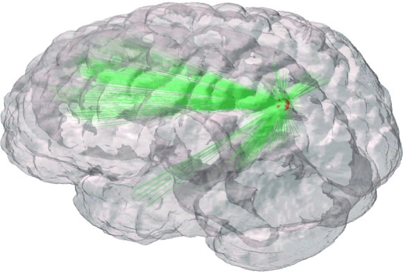
Connections originating from the highest degree node. The highest degree node in a resting-state functional magnetic resonance imaging network is denoted by a sphere. Edges originating from the node, denoted by lines, extend to the brain areas known as the default mode network. Focusing solely on the degree of each node fails to acknowledge the regions to which it is connected. It is important to acknowledge the complex relationship between highly central nodes and the rest of the network.

One of the earliest attempts to compare networks directly, rather than comparing summary metrics, nodal metrics, or edges separately, was the network-based statistic (Zalesky et al., 2010). This method affords more power than a traditional edge-based approach by looking for component-based (connected subgraphs) differences; however, it is also inherently univariate in that the complex topological structure of the network remains unaccounted for. In addition to not accounting for the dependence structure of the networks, these approaches also fail to provide a framework in which the effects of multiple variables of interest and local network features (e.g., disease status, age, race, nodal clustering, nodal centrality, etc.) on the overall network structure can be concurrently examined. In other words, there has yet to be a (non)linear modeling framework developed for brain networks similar to what there has been for fMRI activation data. The exponential random graph model (ERGM) approach of Simpson and associates (2011a, 2011b) allows systematically (multivariately) comparing several local network features (e.g., nodal efficiency, centrality, and other measures just discussed) simultaneously. The ERGM approach can also account for confounding bias similar to the (N,k)-dependence of network measures (i.e., the fact that graph metrics may be influenced by the number of nodes (N) and the average degree (k) of the network) detailed in (van Wijk et al., 2010) and other potential metric interdependencies (Alexander-Bloch et al., 2010; Dorogovtsev et al., 2008). Although this method enables examining the simultaneous effects of multiple local network features on the complex topological structure of the network, it fails to allow assessing the effects of other variables of interest that are not an intrinsic part of the network (e.g., disease status, age, race, etc.) and is currently not able to preserve the networks in brain space. In addition to filling these methodological gaps, future approaches will also need to incorporate connection strength (weighted networks) and/or direction (directed networks) as construction and analysis of these network types gain feasibility. The utility of network comparison tools will likely vary by context; thus, outcomes of interest should inform their development.

When analyzing complex brain networks, one also has to be aware that some of the analyses just described are qualitative rather than quantitative. In a quantitative analysis, one can examine a particular hypothesis by calculating the likelihood for the hypothesis by various statistical methods. Such an analysis often yields a p value describing how unlikely it is to observe the actual data based only on chance. This type of framework suits the traditional philosophy of science, examining whether a hypothesis can be refuted (Popper, 1959). This framework, however, assumes that there is a hypothesis to be tested. This assumption may not be always applicable in network science and other data-intensive fields such as bioinformatics and machine learning; in these fields, a goal of analyses may be simply to describe structures in the data or to uncover hidden patterns among observations. For example, some investigators may be simply interested in topological properties and characteristics, such as information flow, centrality, or community structure, present in their brain network data. The results from such analyses simply describe the network qualitatively (e.g., network communities in the brains of younger and older subjects) and do not yield p values. Of course, it is possible to define a hypothesis for a network analysis (e.g., some nodes have significantly higher degree than others) and to develop a statistical test for that hypothesis. However, such an analysis is only sensitive to detect a departure from that particular hypothesis and cannot describe what is causing that departure. In such a case, one may have to resort to a qualitative description of the network to determine the reason for the departure. For example, Figure 7 shows the highest degree node with many interconnections among areas constituting the default mode network. Focusing on changes in only the node misses the complex relationship that this high centrality node shares with the rest of the network. Although quantitative analyses and p values have been in the mainstream of biomedical research for decades, practitioners of brain network analyses need to be open to a major paradigm shift; many important results in brain network analyses will be qualitative and may not have p values associated with them.

Null Models

For situations where one needs quantitative evaluations of the network, it is vital that an appropriate null model is used for comparison. A random network is often the null model used to study network topology. The most investigated random network model is the Erdős-Rényi (ER) random network (Erdős and Rényi, 1960). Although networks can be compared with an ER model, as seen in Figure 8, the degree distribution of the ER model (Fig. 8B) does not reflect the topology of the network of interest (Fig. 8A), thus complicating its use in analysis. A more common comparison is to generate a random network that shares the same degree distribution as the original network (Maslov and Sneppen, 2002). Preserving the degree distribution in this way is important, because altering the degree distribution as seen in the ER network can potentially confound the network structure. Random network comparison is used in community structure analysis to optimize modularity (Newman and Girvan, 2004). Random networks are also used for quantification of network small-world properties with tight local interconnections and efficient global information transfer. The small-world coefficient σ utilizes a ratio of network clustering and path length compared with its random equivalent (Humphries and Gurney, 2008; Humphries et al., 2006). Although the small-world coefficient is a popular measure of small-worldness, it can be misleading, as the level of clustering in the random network may overstate network small-worldness.

FIG. 8.

Network null models with corresponding degree distribution. In network analysis, null models are used to better assess network topology. (A) The original network (represented as an adjacency matrix and circular graph) is often compared with random network models. Popular random network models include the (B) Erdős-Rényi (ER) random model and the (C) random network with preserved degree distribution. Although less popular, lattice network models can also be used to assess network topology. Null models with preserved degree distribution are generally preferred, as the degree distribution of the ER model does not match that of the original network.

In contrast to using random network models, lattice network models can also be used to evaluate network properties. Sporns and Zwi (2004) developed an algorithm that produces a lattice network with the same degree distribution as the network of interest. Used in conjunction with a random network of the same degree distribution, this allows the scaling of clustering and path length (Sporns and Zwi, 2004). This algorithm has also been used to evaluate network efficiency measures over varying cost (Achard and Bullmore, 2007). In contrast to quantifying small-worldness by comparison to a random network, as done using the small-world coefficient σ, a lattice network can be used to quantify network small-worldness as seen in the small-world measurement ω (Telesford et al., 2011). This metric determines whether a network exhibits simultaneous high clustering with low path length by comparing clustering to a lattice network and path length to a random network.

Conclusions

With the increasing use of network science in neuroimaging, it is becoming more critical to consider the approach to using graph metric tools effectively. Perhaps the greatest issue is the overuse and inappropriate use of average graph metrics or summary statistics to compare networks; although this approach is useful when comparing a network to a null model, using such univariate analyses for group comparisons takes away much of the benefits of network analysis. The rationale for using network science in the brain is to understand the organization and dynamics of the brain as a complex system. Reducing characteristics of a network to a single value renders a poor and often misleading guide for understanding complex systems. Another fundamental problem with such an approach is that measurements within a network are not independent. A measurement at a given node is typically affected by distant nodes. Taking degree as an example, removal of an edge affects two nodes. Likewise, metrics such as clustering coefficient are dependent on the connectivity of neighboring nodes. Slight changes in connectivity patterns can greatly affect the measurements made at a particular node; thus, no nodal measurement in a network is completely independent. This lack of independence renders any analysis based on the central limit theorem inappropriate and naïve. Various studies have reported differences in clustering, path length, and efficiency from a range of diseases and disorders including Alzheimer's disease (Lo et al., 2010; Sanz-Arigita et al., 2010; Yao et al., 2010), multiple sclerosis (He et al., 2009b; Shu et al., 2011), depression (Zhang et al., 2011a), obsessive compulsive disorder (Zhang et al., 2011b), and synesthesia (Hänggi et al., 2011). In two separate studies on epilepsy, one group reported lower path length between patients with epilepsy and the control group (Liao et al., 2010); whereas another study showed an increase (Vlooswijk et al., 2011). Further inquiry to determine the direction of global changes in the network neglects the bigger question: Does the direction of change imply that the network has entered a particular disease state? For example, is lower path length a sign of depression or multiple sclerosis? Although differences can be found using these metrics, their lack of specificity implies that researchers should not rely on global metrics. Due to this, massively univariate analysis methods widely used in functional neuroimaging analyses should not be applied to brain network data.

It may be tempting to summarize the entire network as one number by taking the average metrics that do converge to a normal distribution. However, even comparing summary metrics across the brain may not provide suitable information about a group. Brain networks may share mean clustering, path length, and degree, but the distribution of these metrics across brain space may differ within or across the group. Thus, despite the similar summary metrics, the networks can be massively different. For example, in a study comparing the effects of an exercise regimen in a group of older adults, no significant differences were found for clustering or path length, but the topology of the networks was dramatically different (Burdette et al., 2010). Significant differences in graph metrics can be helpful in determining gross differences between groups, but by and large, a lot of information is lost by reducing the system to a single value. Nonetheless, this does not mean that summary statistics are meaningless, but they should be considered a general starting point for understanding a system. A greater emphasis should be placed on network topology, as examining the organization of the system provides for a better assessment of how a network or group of networks is organized and provides a better route for understanding the complexity of the brain. We also emphasize the importance of qualitative analysis results, such as community structure organization and centrality. Such results often do not yield p values as in quantitative, hypothesis-driven analyses, but investigators can ascertain useful insights into how the brain network is organized.

Analyzing network topology invariably brings up the question of the best approach for network construction. In this area, it seems that weighted network analyses provide the greatest opportunity for exploration. Although some studies suggest that there is not much difference between unweighted and weighted graphs (Li et al., 2009; Ponten et al., 2009), studying the local relationships of nodes can further enhance the understanding of network organization (Saramäki et al., 2007). Another caveat related to weighted networks, especially in functional networks, is that links are based on positive connections, whereas negative connections are ignored. Although some studies include negative links (Chen et al., 2011; Schwarz and McGonigle, 2011), there is still a problem with the conceptualization of negative links in relation to different graph metrics, such as clustering coefficient. In a recent study by Rubinov and Sporns (2011), a weighted network including negative links was analyzed without an applied threshold. Although the inclusion of negative weights should be considered, we feel that it is best to threshold the network to generate sparse connectivity to best capture the true topology of the brain. However, it should be emphasized that the most appropriate method to eliminate spurious links has yet to be developed.

As the field of network science continues to grow, it will continue to gain greater popularity in the neuroimaging field. At many scientific conferences, network science approaches to brain imaging have increased significantly with more posters, lectures, and symposia becoming more commonplace. With the prospect of such growth, we want to emphasize the importance of using graph theory effectively and appropriately within a new framework of thinking about the brain—complexity, as linear thinking is a poor guide for understanding complex systems. There is already a trend in network neuroimaging whereby neuroscientists download the latest “network analysis” tools, apply these tools to an fMRI dataset, get summary global statistics, and then believe they are uncovering/understanding complexity-based aspects of the brain. We believe that this attitude represents a missed opportunity, as the brain cannot be summarized by a single number; in order to fully appreciate the power of network science in the brain, a novel way of thinking should be adopted in order to fully appreciate these complexity-based approaches. Use of network science requires an approach that is less geared toward reductionism (i.e., reducing a system to its smaller constituent parts) and more toward complexity and how interactions in the network drive the system. The power of network science stems from its ability to capture these dynamics, which will play an important role in understanding the brain as a complex system.

Author Disclosure Statement

No competing financial interests exist.

References

- Achard S. Bullmore E. Efficiency and cost of economical brain functional networks. PLoS Comput Biol. 2007;3:e17. doi: 10.1371/journal.pcbi.0030017. [DOI] [PMC free article] [PubMed] [Google Scholar]
- Achard S. Salvador R. Whitcher B. Suckling J. Bullmore E. A resilient, low-frequency, small-world human brain functional network with highly connected association cortical hubs. J Neurosci. 2006;26:63–72. doi: 10.1523/JNEUROSCI.3874-05.2006. [DOI] [PMC free article] [PubMed] [Google Scholar]
- Alexander-Bloch AF, et al. Disrupted modularity and local connectivity of brain functional networks in childhood-onset schizophrenia. Front Syst Neurosci. 2010;4:147. doi: 10.3389/fnsys.2010.00147. [DOI] [PMC free article] [PubMed] [Google Scholar]
- Balenzuela P, et al. Modular organization of brain resting state networks in chronic back pain patients. Front Neuroinform. 2010;4:116. doi: 10.3389/fninf.2010.00116. [DOI] [PMC free article] [PubMed] [Google Scholar]
- Bassett DS, et al. Hierarchical organization of human cortical networks in health and schizophrenia. J Neurosci. 2008;28:9239–9248. doi: 10.1523/JNEUROSCI.1929-08.2008. [DOI] [PMC free article] [PubMed] [Google Scholar]
- Bassett DS, et al. Dynamic reconfiguration of human brain networks during learning. Proc Natl Acad Sci U S A. 2011;108:7641–7646. doi: 10.1073/pnas.1018985108. [DOI] [PMC free article] [PubMed] [Google Scholar]
- Bavelas A. A mathematical model of group structures. Hum Organ. 1948;7:16–30. [Google Scholar]
- Beggs JM. Plenz D. Neuronal avalanches in neocortical circuits. J Neurosci. 2003;23:11167–11177. doi: 10.1523/JNEUROSCI.23-35-11167.2003. [DOI] [PMC free article] [PubMed] [Google Scholar]
- Bonacich P. Power and centrality: a family of measures. Am J Sociol. 1987;92:1170–1182. [Google Scholar]
- Borgatti SP. Centrality and network flow. Soc Networks. 2005;27:55–71. [Google Scholar]
- Borgatti SP. Everett MG. A Graph-theoretic perspective on centrality. Soc Networks. 2006;28:466–484. [Google Scholar]
- Buckner RL, et al. Cortical hubs revealed by intrinsic functional connectivity: Mapping, assessment of stability, and relation to Alzheimer's disease. J Neurosci. 2009;29:1860–1873. doi: 10.1523/JNEUROSCI.5062-08.2009. [DOI] [PMC free article] [PubMed] [Google Scholar]
- Bullmore E. Sporns O. Complex brain networks: graph theoretical analysis of structural and functional systems. Nat Rev Neurosci. 2009;10:186–198. doi: 10.1038/nrn2575. [DOI] [PubMed] [Google Scholar]
- Burdette JH, et al. Using network science to evaluate exercise-associated brain changes in older adults. Front Aging Neurosci. 2010;2:23. doi: 10.3389/fnagi.2010.00023. [DOI] [PMC free article] [PubMed] [Google Scholar]
- Chen G. Chen G. Xie C. Li S.-J. Negative functional connectivity and its dependence on the shortest path length of positive network in the resting-state human brain. Brain Connectivity. 2011;1:195–206. doi: 10.1089/brain.2011.0025. [DOI] [PMC free article] [PubMed] [Google Scholar]
- Dorogovtsev SN. Mendes JFF. Samukhin AN. Zyuzin AY. Organization of modular networks. Phys Rev E Stat Nonlin Soft Matter Phys. 2008;78:056106. doi: 10.1103/PhysRevE.78.056106. [DOI] [PubMed] [Google Scholar]
- Drachman DA. Do we have brain to spare? Neurology. 2005;64:2004–2005. doi: 10.1212/01.WNL.0000166914.38327.BB. [DOI] [PubMed] [Google Scholar]
- Eguíluz VM. Chialvo DR. Cecchi GA. Baliki M. Apkarian AV. Scale-free brain functional networks. Phys Rev Lett. 2005;94:018102. doi: 10.1103/PhysRevLett.94.018102. [DOI] [PubMed] [Google Scholar]
- Erdős P. Rényi A. On the evolution of random graphs. Publ Math Inst Hung Acad Sci. 1960;5:17–61. [Google Scholar]
- Fortunato S. Community detection in graphs. Phys Rep. 2010;486:75–174. [Google Scholar]
- Fortunato S. Barthélemy M. Resolution limit in community detection. Proc Natl Acad Sci U S A. 2007;104:36–41. doi: 10.1073/pnas.0605965104. [DOI] [PMC free article] [PubMed] [Google Scholar]
- Fox MD, et al. The human brain is intrinsically organized into dynamic, anticorrelated functional networks. Proc Natl Acad Sci U S A. 2005;102:9673–9678. doi: 10.1073/pnas.0504136102. [DOI] [PMC free article] [PubMed] [Google Scholar]
- Freeman L. A set of measures of centrality based on betweenness. Sociometry. 1977;40:35–41. [Google Scholar]
- Freeman L. Centrality in social networks: conceptual clarification. Soc Networks. 1979;1:215–239. [Google Scholar]
- Gavin A-C, et al. Functional organization of the yeast proteome by systematic analysis of protein complexes. Nature. 2002;415:141–147. doi: 10.1038/415141a. [DOI] [PubMed] [Google Scholar]
- Girvan M. Newman MEJ. Community structure in social and biological networks. Proc Natl Acad Sci U S A. 2002;99:7821–7826. doi: 10.1073/pnas.122653799. [DOI] [PMC free article] [PubMed] [Google Scholar]
- Gong G, et al. Mapping anatomical connectivity patterns of human cerebral cortex using in vivo diffusion tensor imaging tractography. Cereb Cortex. 2009;19:524–536. doi: 10.1093/cercor/bhn102. [DOI] [PMC free article] [PubMed] [Google Scholar]
- Guimerà R. Amaral LA. Functional cartography of complex metabolic networks. Nature. 2005;433:895–900. doi: 10.1038/nature03288. [DOI] [PMC free article] [PubMed] [Google Scholar]
- Guimerà R. Sales-Pardo M. Amaral LA. Classes of complex networks defined by role-to-role connectivity profiles. Nat Phys. 2007;3:63–69. doi: 10.1038/nphys489. [DOI] [PMC free article] [PubMed] [Google Scholar]
- Hagmann P, et al. Mapping the structural core of human cerebral cortex. PLoS Biol. 2008;6:e159. doi: 10.1371/journal.pbio.0060159. [DOI] [PMC free article] [PubMed] [Google Scholar]
- Hänggi J. Wotruba D. Jäncke L. Globally altered structural brain network topology in grapheme-color synesthesia. J Neurosci. 2011;31:5816–5828. doi: 10.1523/JNEUROSCI.0964-10.2011. [DOI] [PMC free article] [PubMed] [Google Scholar]
- Hayasaka S. Laurienti PJ. Comparison of characteristics between region-and voxel-based network analyses in resting-state fMRI data. NeuroImage. 2010;50:499–508. doi: 10.1016/j.neuroimage.2009.12.051. [DOI] [PMC free article] [PubMed] [Google Scholar]
- He Y. Chen ZJ. Evans AC. Small-world anatomical networks in the human brain revealed by cortical thickness from MRI. Cereb Cortex. 2007;17:2407–2419. doi: 10.1093/cercor/bhl149. [DOI] [PubMed] [Google Scholar]
- He Y. Chen Z. Evans A. Structural insights into aberrant topological patterns of large-scale cortical networks in Alzheimer's disease. J Neurosci. 2008;28:4756–4766. doi: 10.1523/JNEUROSCI.0141-08.2008. [DOI] [PMC free article] [PubMed] [Google Scholar]
- He Y, et al. Uncovering intrinsic modular organization of spontaneous brain activity in humans. PLoS ONE. 2009a;4:e5226. doi: 10.1371/journal.pone.0005226. [DOI] [PMC free article] [PubMed] [Google Scholar]
- He Y, et al. Impaired small-world efficiency in structural cortical networks in multiple sclerosis associated with white matter lesion load. Brain. 2009b;132:3366–3379. doi: 10.1093/brain/awp089. [DOI] [PMC free article] [PubMed] [Google Scholar]
- Honey CJ. Kötter R. Breakspear M. Sporns O. Network structure of cerebral cortex shapes functional connectivity on multiple time scales. Proc Natl Acad Sci U S A. 2007;104:10240–10245. doi: 10.1073/pnas.0701519104. [DOI] [PMC free article] [PubMed] [Google Scholar]
- Honey CJ, et al. Predicting human resting-state functional connectivity from structural connectivity. Proc Natl Acad Sci U S A. 2009;106:2035–2040. doi: 10.1073/pnas.0811168106. [DOI] [PMC free article] [PubMed] [Google Scholar]
- Humphries MD. Gurney K. Network ‘small-world-ness’: a quantitative method for determining canonical network equivalence. PLoS ONE. 2008;3:e0002051. doi: 10.1371/journal.pone.0002051. [DOI] [PMC free article] [PubMed] [Google Scholar]
- Humphries MD. Gurney K. Prescott TJ. The brainstem reticular formation is a small-world, not scale-free, network. Proc Biol Sci. 2006;273:503–511. doi: 10.1098/rspb.2005.3354. [DOI] [PMC free article] [PubMed] [Google Scholar]
- Iturria-Medina Y. Sotero RC. Canales-Rodríguez EJ. Alemán-Gómez Y. Melie-García L. Studying the human brain anatomical network via diffusion-weighted MRI and graph theory. NeuroImage. 2008;40:1064–1076. doi: 10.1016/j.neuroimage.2007.10.060. [DOI] [PubMed] [Google Scholar]
- Jouve B. Rosenstiehl P. Imbert M. A mathematical approach to the connectivity between the cortical visual areas of the macaque monkey. Cereb Cortex. 1998;8:28–39. doi: 10.1093/cercor/8.1.28. [DOI] [PubMed] [Google Scholar]
- Joyce KE. Laurienti PJ. Burdette JH. Hayasaka S. A new measure of centrality for brain networks. PLoS ONE. 2010;5:e12200. doi: 10.1371/journal.pone.0012200. [DOI] [PMC free article] [PubMed] [Google Scholar]
- Kovács IA. Palotai R. Szalay MS. Csermely P. Community landscapes: an integrative approach to determine overlapping network module hierarchy, identify key nodes and predict network dynamics. PLoS ONE. 2010;5:e12528. doi: 10.1371/journal.pone.0012528. [DOI] [PMC free article] [PubMed] [Google Scholar]
- Kumpula JM, et al. Emergence of communities in weighted networks. Phys Rev Lett. 2007;99:228701. doi: 10.1103/PhysRevLett.99.228701. [DOI] [PubMed] [Google Scholar]
- Lancichinetti A. Radicchi F. Ramasco JJ. Fortunato S. Finding statistically significant communities in networks. PLoS ONE. 2011;6:e18961. doi: 10.1371/journal.pone.0018961. [DOI] [PMC free article] [PubMed] [Google Scholar]
- Laurienti PJ. Joyce KE. Telesford QK. Burdette JH. Hayasaka S. Universal fractal scaling of self-organized networks. Physica A. 2011;390:3608–3613. doi: 10.1016/j.physa.2011.05.011. [DOI] [PMC free article] [PubMed] [Google Scholar]
- Li Y, et al. Brain anatomical network and intelligence. PLoS Comput Biol. 2009;5:e1000395. doi: 10.1371/journal.pcbi.1000395. [DOI] [PMC free article] [PubMed] [Google Scholar]
- Liao W, et al. Altered functional connectivity and small-world in mesial temporal lobe epilepsy. PLoS ONE. 2010;5:e8525. doi: 10.1371/journal.pone.0008525. [DOI] [PMC free article] [PubMed] [Google Scholar]
- Lo C-Y, et al. Diffusion tensor tractography reveals abnormal topological organization in structural cortical networks in Alzheimer's disease. J Neurosci. 2010;30:16876–16885. doi: 10.1523/JNEUROSCI.4136-10.2010. [DOI] [PMC free article] [PubMed] [Google Scholar]
- Lohmann G, et al. Eigenvector centrality mapping for analyzing connectivity patterns in fMRI data of the human brain. PLoS ONE. 2010;5:e10232. doi: 10.1371/journal.pone.0010232. [DOI] [PMC free article] [PubMed] [Google Scholar]
- Lynall M-E, et al. Functional connectivity and brain networks in schizophrenia. J Neurosci. 2010;30:9477–9487. doi: 10.1523/JNEUROSCI.0333-10.2010. [DOI] [PMC free article] [PubMed] [Google Scholar]
- Maslov S. Sneppen K. Specificity and stability in topology of protein networks. Science. 2002;296:910–913. doi: 10.1126/science.1065103. [DOI] [PubMed] [Google Scholar]
- Mason O. Verwoerd M. Graph theory and networks in biology. IET Syst Biol. 2007;1:89–119. doi: 10.1049/iet-syb:20060038. [DOI] [PubMed] [Google Scholar]
- Meunier D. Lambiotte R. Fornito A. Ersche K. Bullmore ET. Hierarchical modularity in human brain functional networks. Front Neuroinform. 2009;3:37. doi: 10.3389/neuro.11.037.2009. [DOI] [PMC free article] [PubMed] [Google Scholar]
- Micheloyannis S, et al. Using graph theoretical analysis of multi channel EEG to evaluate the neural efficiency hypothesis. Neurosci Lett. 2006;402:273–277. doi: 10.1016/j.neulet.2006.04.006. [DOI] [PubMed] [Google Scholar]
- Moussa MN, et al. Changes in cognitive state alter human functional brain networks. Front in Hum Neurosci. 2011;5:83. doi: 10.3389/fnhum.2011.00083. [DOI] [PMC free article] [PubMed] [Google Scholar]
- Mucha PJ. Richardson T. Macon K. Porter MA. Onnela J-P. Community structure in time-dependent, multiscale, and multiplex networks. Science. 2010;328:876–878. doi: 10.1126/science.1184819. [DOI] [PubMed] [Google Scholar]
- Newman MEJ. Finding community structure in networks using the eigenvectors of matrices. Phys Rev E Stat Nonlin Soft Matter Phys. 2006;74:036104. doi: 10.1103/PhysRevE.74.036104. [DOI] [PubMed] [Google Scholar]
- Newman MEJ. Girvan M. Finding and evaluating community structure in networks. Phys Rev E Stat Nonlin Soft Matter Phys. 2004;69:026113. doi: 10.1103/PhysRevE.69.026113. [DOI] [PubMed] [Google Scholar]
- Palla G. Derenyi I. Farkas I. Vicsek T. Uncovering the overlapping community structure of complex networks in nature and society. Nature. 2005;435:814–818. doi: 10.1038/nature03607. [DOI] [PubMed] [Google Scholar]
- Petrella JR. Use of graph theory to evaluate brain networks: a clinical tool for a small world? Radiology. 2011;259:317–320. doi: 10.1148/radiol.11110380. [DOI] [PubMed] [Google Scholar]
- Ponten SC. Douw L. Bartolomei F. Reijneveld JC. Stam CJ. Indications for network regularization during absence seizures: weighted and unweighted graph theoretical analyses. Exp Neurol. 2009;217:197–204. doi: 10.1016/j.expneurol.2009.02.001. [DOI] [PubMed] [Google Scholar]
- Popper KR. The Logic of Scientific Discovery. NY: Basic Books; 1959. pp. 57–73. [Google Scholar]
- Rivière D, et al. Automatic recognition of cortical sulci of the human brain using a congregation of neural networks. Med Image Anal. 2002;6:77–92. doi: 10.1016/s1361-8415(02)00052-x. [DOI] [PubMed] [Google Scholar]
- Ruan J. Zhang W. Identifying network communities with a high resolution. Phys Rev E Stat Nonlin Soft Matter Phys. 2008;77:016104. doi: 10.1103/PhysRevE.77.016104. [DOI] [PubMed] [Google Scholar]
- Rubinov M. Sporns O. Complex network measures of brain connectivity: uses and interpretations. NeuroImage. 2010;52:1059–1069. doi: 10.1016/j.neuroimage.2009.10.003. [DOI] [PubMed] [Google Scholar]
- Rubinov M. Sporns O. Weight-conserving characterization of complex functional brain networks. NeuroImage. 2011;56:2068–2079. doi: 10.1016/j.neuroimage.2011.03.069. [DOI] [PubMed] [Google Scholar]
- Sanz-Arigita EJ, et al. Loss of ‘small-world’; networks in Alzheimer's disease: graph analysis of fMRI resting-state functional connectivity. PLoS ONE. 2010;5:e13788. doi: 10.1371/journal.pone.0013788. [DOI] [PMC free article] [PubMed] [Google Scholar]
- Saramäki J. Kivelä M. Onnela J-P. Kaski K. Kertész J. Generalizations of the clustering coefficient to weighted complex networks. Phys Rev E Stat Nonlin Soft Matter Phys. 2007;75:027105. doi: 10.1103/PhysRevE.75.027105. [DOI] [PubMed] [Google Scholar]
- Schwarz AJ. McGonigle J. Negative edges and soft thresholding in complex network analysis of resting state functional connectivity data. NeuroImage. 2011;55:1132–1146. doi: 10.1016/j.neuroimage.2010.12.047. [DOI] [PubMed] [Google Scholar]
- Shu N, et al. Diffusion tensor tractography reveals disrupted topological efficiency in white matter structural networks in multiple sclerosis. Cereb Cortex. 2011;21:2565–2577. doi: 10.1093/cercor/bhr039. [DOI] [PubMed] [Google Scholar]
- Simpson SL. Hayasaka S. Laurienti PJ. Exponential random graph modeling for complex brain networks. PLoS ONE. 2011a;6:e20039. doi: 10.1371/journal.pone.0020039. [DOI] [PMC free article] [PubMed] [Google Scholar]
- Simpson SL. Moussa MN. Laurienti PJ. An exponential random graph modeling approach to creating group-based representative whole-brain connectivity networks. 2011b. arXiv:1101.2592v1 [stat.AP]. [DOI] [PMC free article] [PubMed]
- Sporns O. Honey CJ. Kötter R. Identification and classification of hubs in brain networks. PLoS ONE. 2007;2:e1049. doi: 10.1371/journal.pone.0001049. [DOI] [PMC free article] [PubMed] [Google Scholar]
- Sporns O. Tononi G. Edelman GM. Theoretical neuroanatomy and the connectivity of the cerebral cortex. Behav Brain Res. 2002;135:69–74. doi: 10.1016/s0166-4328(02)00157-2. [DOI] [PubMed] [Google Scholar]
- Sporns O. Tononi G. Kötter R. The human connectome: a structural description of the human brain. PLoS Comput Biol. 2005;1:e42. doi: 10.1371/journal.pcbi.0010042. [DOI] [PMC free article] [PubMed] [Google Scholar]
- Sporns O. Zwi J. The small world of the cerebral cortex. Neuroinformatics. 2004;2:145–162. doi: 10.1385/NI:2:2:145. [DOI] [PubMed] [Google Scholar]
- Srinivas KV. Jain R. Saurav S. Sikdar SK. Small-world network topology of hippocampal neuronal network is lost, in an in vitro glutamate injury model of epilepsy. Eur J Neurosci. 2007;25:3276–3286. doi: 10.1111/j.1460-9568.2007.05559.x. [DOI] [PubMed] [Google Scholar]
- Stam C. Jones B. Nolte G. Breakspear M. Scheltens P. Small-world networks and functional connectivity in Alzheimer's disease. Cereb Cortex. 2007;17:92–99. doi: 10.1093/cercor/bhj127. [DOI] [PubMed] [Google Scholar]
- Stam CJ. Functional connectivity patterns of human magnetoencephalographic recordings: a 'small-world' network? Neurosci Lett. 2004;355:25–28. doi: 10.1016/j.neulet.2003.10.063. [DOI] [PubMed] [Google Scholar]
- Steen M. Hayasaka S. Joyce K. Laurienti P. Assessing the consistency of community structure in complex networks. Phys Rev E Stat Nonlin Soft Matter Phys. 2011;84:016111. doi: 10.1103/PhysRevE.84.016111. [DOI] [PMC free article] [PubMed] [Google Scholar]
- Südhof TC. The synaptic vesicle cycle. Annu Rev Neurosci. 2004;27:509–547. doi: 10.1146/annurev.neuro.26.041002.131412. [DOI] [PubMed] [Google Scholar]
- Telesford QK. Joyce KE. Hayasaka S. Burdette JH. Laurienti PJ. The ubiquity of small-world networks. 2011. arXiv (arXiv:1109.5454v1) [nlin.AO]. [DOI] [PMC free article] [PubMed]
- Tzourio-Mazoyer N, et al. Automated anatomical labeling of activations in SPM using a macroscopic anatomical parcellation of the MNI MRI single-subject brain. NeuroImage. 2002;15:273–289. doi: 10.1006/nimg.2001.0978. [DOI] [PubMed] [Google Scholar]
- van den Heuvel MP. Stam CJ. Boersma M. Hulshoff Pol HE. Small-world and scale-free organization of voxel-based resting-state functional connectivity in the human brain. NeuroImage. 2008;43:528–539. doi: 10.1016/j.neuroimage.2008.08.010. [DOI] [PubMed] [Google Scholar]
- van Wijk BCM. Stam CJ. Daffertshofer A. Comparing brain networks of different size and connectivity density using graph theory. PLoS ONE. 2010;5:e13701. doi: 10.1371/journal.pone.0013701. [DOI] [PMC free article] [PubMed] [Google Scholar]
- Vlooswijk MCG, et al. Loss of network efficiency associated with cognitive decline in chronic epilepsy. Neurology. 2011;77:938–944. doi: 10.1212/WNL.0b013e31822cfc2f. [DOI] [PubMed] [Google Scholar]
- Wang J, et al. Parcellation-dependent small-world brain functional networks: a resting-state fMRI study. Hum Brain Mapp. 2009;30:1511–1523. doi: 10.1002/hbm.20623. [DOI] [PMC free article] [PubMed] [Google Scholar]
- Watts DJ. Strogatz SH. Collective dynamics of ‘small-world' networks. Nature. 1998;393:440–442. doi: 10.1038/30918. [DOI] [PubMed] [Google Scholar]
- Wilson RJ. Introduction to Graph Theory. 4th. Upper Saddle River, NJ: Prentice Hall; 1996. p. 26. [Google Scholar]
- Wu K, et al. The overlapping community structure of structural brain network in young healthy individuals. PLoS ONE. 2011;6:e19608. doi: 10.1371/journal.pone.0019608. [DOI] [PMC free article] [PubMed] [Google Scholar]
- Yao Z, et al. Abnormal cortical networks in mild cognitive impairment and Alzheimer's disease. PLoS Comput Biol. 2010;6:e1001006. doi: 10.1371/journal.pcbi.1001006. [DOI] [PMC free article] [PubMed] [Google Scholar]
- Zalesky A. Fornito A. Bullmore ET. Network-based statistic: identifying differences in brain networks. NeuroImage. 2010;53:1197–1207. doi: 10.1016/j.neuroimage.2010.06.041. [DOI] [PubMed] [Google Scholar]
- Zamora-López G. Zhou C. Kurths J. Graph analysis of cortical networks reveals complex anatomical communication substrate. Chaos. 2009;19:015117. doi: 10.1063/1.3089559. [DOI] [PubMed] [Google Scholar]
- Zhang J, et al. Disrupted brain connectivity networks in drug-naive, first-episode major depressive disorder. Biol Psychiatry. 2011a;70:334–342. doi: 10.1016/j.biopsych.2011.05.018. [DOI] [PubMed] [Google Scholar]
- Zhang T, et al. Abnormal small-world architecture of top-down control networks in obsessive-compulsive disorder. J Psychiatry Neurosci. 2011b;36:23–31. doi: 10.1503/jpn.100006. [DOI] [PMC free article] [PubMed] [Google Scholar]