An in situ Measurement of Extracellular Cysteamine, Homocysteine and Cysteine Concentrations in Organotypic Hippocampal Slice Cultures by Integration of Electroosmotic Sampling and Microfluidic Analysis

Abstract

We demonstrate an all-electric sampling/derivatization/separation/detection system for the quantitation of thiols in tissue cultures. Extracellular fluid collected from rat organotypic hippocampal slice cultures (OHSCs) by electroosmotic flow through an11 cm (length) × 50 μm (ID) sampling capillary is introduced to a simple microfluidic chip for derivatization, continuous flow-gated injection, separation and detection.With the help of a fluorogenic, thiol-specific reagent, ThioGlo-1, we have successfully separated and detected the extracellular levels of free reduced cysteamine, homocysteineand cysteinefrom OHSCs within 25 s in a 23 mm separation channel with a confocal laser induced fluorescence (LIF) detector. Attention to the conductivities of the fluids being transported is required for successful flow-gated injections.When the sample conductivity is much higher than the run buffer conductivities, the electroosmotic velocities are such that there is less fluid coming by electroosmosis into the cross from the sample/reagent channel than is leaving by electroosmosis into the separation and waste channels. The resulting decrease in the internal fluid pressure in the injection cross pulls flow from the gated channel. This process may completely shut down the gated injection. Using a glycylglycine buffer with physiological osmolarity but only 62% of physiological conductivity and augmenting the conductivity of the run buffers solved this problem. Quantitation is by standard additions. Concentrations of cysteamine, homocysteine and cysteine in the extracellular space of OHSCs are10.6±1.0 nM (n=70), 0.18±0.01 μM (n=53) and 11.1±1.2 μM (n=70), respectively. This is the first in situquantitative estimation of endogenous cysteamine in brain. Extracellular levels of homocysteine and cysteine are comparable with other reported values.

The coupling of sample collection and microfluidic analysis addresses the critical problems that arise in handling small amounts of liquid samples.¹Several groups have devised useful approachesto transport samples from cells, tissues, or living animals directly to a microfluidic chip for online analysis.^2-5But to the best of our knowledge all the published methods require extra vacuum/pressure pumps for transporting the samples either from a push-pull perfusion probe² or a microdialysis probe^3-5 to the microfluidic chip for further analysis. The addition of these pumps increases the total cost and the complexity of the system.

Electroosmosis is the natural and dominant driving force incapillary electrophoresis (CE) and microfluidic chips.^6-7Electroosmosis requires no mechanical pumps but can generate accurate flow rates in the domain of less than one to tens of nL/s depending on the cross sectional area of the conduit.⁸In addition, the plug shaped electroosmotic flow creates less solute dispersion than that of parabolic flow in a pressure-driven system. Under an external electric field, solvated cations in the diffuse layer will migrate towards the cathode,dragging the bulk solution. The potential at the shear boundary of the fluid defines the ζ-potential that governs the electroosmotic flow (EOF). Under physiological conditions, the cell surface is naturally negatively charged like that of the wall in a fused silica capillary or a microfluidic channel.⁹We have reported that OHSCs have a ζ-potential of −22.8 mV,¹⁰ therefore the EOF generated with an electric field can be used to pump the extracellular fluid out of the tissue for analysis. Our lab has developed an EO sampling method to extract extracellular fluid from organotypic hippocampal slice cultures(OHSCs)into a fused silica capillary. In that work, the sample inside the capillary was then collected for offline HPLC analysis.¹¹

Cysteine,homocysteineand cysteamine arethree related aminothiolsthatexist in tissues and body fluids at low levels.^12-13Although cysteineis neurotoxic,¹⁴ it is a rate-limitingsynthetic precursor of glutathione in neurons. The latter plays a critical role in defending cells against oxidative stress.¹⁵In brain, neuronal glutathione synthesis relies oncysteine that arises from extracellular hydrolysis of glutathione exportedfrom astroglia by γ-glutamyl transpeptidaseand aminopeptidase N.This interplay results in an intensive metabolic exchange with astrocytes.¹⁶The cysteine concentration in plasma is estimated to be in the range of 8-10 μM,¹⁷ while the concentration of cysteine in the extracellular space of rat caudate nucleus and striatum determined by microdialysis is round 2 μM.^18-19 Cysteine at 1 mM concentration is the killing threshold via NMDA receptors.¹⁴Homocysteine is an important endogenous molecule in the metabolism of methionine, and it connects the methionine and cysteinemetabolic cycles.¹²Onlytrace amounts (0.05-0.3 μM) of free homocysteine (1-2% of total homocysteine) exist in its reduced form in plasma.²⁰Changes in the levels of cysteine/homocysteine or their oxidized formsin biological systems usually indicate dysfunctions of related metabolic cycles or cellular processes.Specifically, cystinosisis due to accumulation of abnormal amountsof cystine in lysosomes.²¹The homocysteine level in plasma/serum is considered to bea biomarker of clinical disorders, such as Alzheimer’s disease and cardiovascular disease.¹²Due to their importance, numerous methods have been developed to detect and quantify free or total cysteine and homocysteine in body fluids such as plasma,^22-24urine,^{23, 25}tissue homogenates,²⁶whilefewer studies have been done on the extracellular space of tissues^18-19 through microdialysis.The dominant quantitation methods are HPLC or capillary electrophoresis equipped with UV, fluorescence (FL) or mass spectrometry detectors.^27-28

Although cysteamine is a decarboxylated form of cysteine, itis widely believed to be the active terminal product of thesynthesis and degradation of coenzyme A in the cysteine metabolic cycle.²⁹ Although cysteamine existsat a very low concentration in the tissue,³⁰itsoxidationis believed to be an indispensablepathway for taurine synthesis, the second most abundant amino acid in mammalian tissues.³¹Cysteamine hasmany otherremarkable roles and biological functions. As an FDA-approved drug for treating cystinosis, cysteaminecan cross the lysosome membrane, react withthe cystine to form a mixed disulfide which can be transported out of the lysosome.³²In addition to its potent radio-protective action onDNA-induced radiation damage,cysteamine, as well as its oxidized form cystamine, have been considered as potential neuroprotective agents. Both compounds have shown significant beneficial properties in treating models of neurodegenerative disease, such as Huntington’s and Parkinson’s diseases.³³Measuring the cysteamine concentration in biological samples is vital for understanding its metabolic mechanism and fate.Endogenous cysteamine levels in different tissue homogenates(brain,liver, kidney, etc),^34-40 urine and plasma^{23, 39, 41} have been reportedusing HPLC-electrochemical detection^36-38/fluorescence^{35-36, 39-41},and CE-LIF²³.Thepublished values cover a very wide range, which ismostlikely due to the inadequate methodologyas well as species differences.^{30, 38}Several workers report that the endogenousconcentration of free cysteaminein brain tissue homogenates is very low and below the detection limits of the most sensitive detection methods(<10 nmol/L).^{30, 35, 38-39}We are unaware of measurements in vivo or in in vitro preparations such as acute or cultured brain slices.

In this work, we integrated online EO sampling and microfluidic analysis coupled to confocal LIF detection to evaluate the endogenous free cysteine, homocysteine and cysteamineconcentrations in the extracellular space of OHSCs. Compared with publicationscited above, the method described here is faster, more sensitive; and to the best of our knowledge for the first time simultaneously evaluates the endogenous cysteine, homocysteine and cysteaminein the extracellular space of any tissue.

EXPERIMENTAL SECTION

Chemicals and Reagents

Tris (hydroxymethyl)aminomethane(Tris base), 1,3-bis[tris(hydroxymethyl)methylamino]propane(Bis-Tris propane),hydrochloric acid, sodium hydroxide, dimethyl sulfoxideanhydrous (DMSO), D-(+)-glucose, glycylglycine, L-cysteine, DL-homocysteine, cysteamine hydrochloride, Gey’s balance salt solution (GBSS)and nitric acid (70%) were purchased from Sigma-Aldrich Chemical Co. (St. Louis, MO).Hydrofluoric acid (48-50%) was fromFisher Scientific (Pittsburgh, PA). Sodium chloride,potassium chloride and methanolwere obtained from Avantor Performance Materials (Center Valley, PA). Potassium phosphate monobasic and calcium chloride dihydrate werefrom EM Science (Gibbstown, NJ). Opti-MEM, horse serum, propidium iodide (PI), and Hank’s balanced salt solution (HBSS) with phenol redwere from Life Technologies (Grand Island, NY).ThioGlo-1, sodium bicarbonate and anhydrous magnesium sulfate were purchased from EMD Millipore (Billerica, MA).

Stock solutions ofcysteamine,homocysteine and cysteinewere prepared no more than two days before experimentsusing degassed Milli-Q water (EMD Millipore) and stored at −20 °C. The final concentrations of these solutions were 120.0 mM, 69.1 mM and 49.7 mM, individually. The stock solution of ThioGlo-1 was prepared using anhydrous DMSO with the final concentration of 2.5 mM. Stock solutions were diluted serially to the desired concentration during the experiments and kept on dry ice when not in use. The artificial cerebrospinal fluid (ACSF) was composed of 128 mM NaCl, 3 mM KCl, 2 mM CaCl₂, 1.2 mM MgSO₄, 0.4 mM KH₂PO₄, 25 mM NaHCO₃ and 10 mM D-glucose.⁴²Glycylglycinemodified ACSF (ggACSF) was prepared by replacing 75 mM NaCl in ACSF with 125 mM glycylglycine and keeping all other components unchanged. Both solutions were adjusted to pH7.40 using NaOH. GBSS used during sampling experiments was fortified with 2.7 mM MgSO4 and 0.5% D-(+)-glucose.The term GBSS used below means “fortified GBSS” unless otherwise specified.PI solution was prepared using GBSS to a final concentration of 0.35 mM and was stored in the freezer. For microfluidic chip electrophoresis, the run buffer was 40 mM Bis-Tris propane buffer with 15 mM NaCl (pH8.50) unless otherwise specified. Tris-HCl buffer (20 mM, pH7.50)was used as the derivatizing buffer for the thiol analytes. All buffers were filtered through 0.1 μm polyethersulfone membrane (EMD Millipore) and degassed by ultrasonication prior to use.

Design of a Microfluidic Chip Coupled withElectroosmotic Sampling

The AZ 1500 photoresist coated borofloat glassplates (Telic, Valencia, CA) for the microfluidic chipswere treated using traditional lithography techniques as described previously.⁴³Briefly, after UV exposure, development and removal of the underlying chromium layer, the glass plate was etched (HF/HNO₃:200/30 (v/v)) to a desired depth (Caution! HF is harmful both through the vapor phase and as a liquid. Its effects may be acute or chronic. Calcium gluconte gel should be on hand before using HF. Consult local standard operating procedures before using HF). The photoresist and chromium remaining on the platewerethen removed completely. The etched glass plate was carefully aligned with another uncoated borofloat cover plate pre-drilled with liquid access holes. Permanent bonding between two plates was achieved by annealing at 655 °C for 8 hours. The mask width for all channels is 30 μm and the etching depth is 20 μm. Figure 1 shows the layout of the microfluidic chip and the coupling of electroosmotic sampling with microfluidic analysis.The total length of the reaction channel from the mixing junction to the injection cross is ~46.3 mm. The detection point (DP) is about 23 mm away from the injection cross. R1, R2, R3 and R4 represent derivatizing reagent reservoir, buffer reservoir, waste reservoir and auxiliary reservoir, respectively. An11 cm (length) ×50 μm (ID)/360 μm (OD)fused silica capillary tube (Polymicro Technologies, Phoenix, AZ)was connected to the R5 through a NanoPort™ assembly (IDEX Health&Science LLC, Oak Harbor, WA).The free tip of the capillary was positioned by a Sutter MP-285 micromanipulator system (Sutter Instrument Company, Novato, CA) near the surface of an OHSC. Platinum electrodes (0.5 mm diameter, Goodfellow Corporation, Oakdale, PA) made electrical contact with solutions in all reservoirs and the Petri dish (35×10 mm, BD, Franklin Lakes, NJ).During the experiment, the electrodes in R1 and the Petri dish were connected to positive power supplies (UltraVolt, Inc., Ronkonkoma, NY). The electrode in R3 was connected to a negative power supply, while the one in R4 was kept at ground (GND). Flow-gated sampling was achieved through the switchingof electrode in R2between the “GND” (separation) and “floating” (injection) states.Extra caution is required when working with high voltage power supplies. All voltages were controlled remotely by computer.

Figure 1.

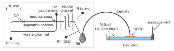
Layout of the microfluidic chip for online EO sampling and microfluidic analysis.

Instrumentation

Detection was achieved through a home-made LIF detector.⁴³Briefly, a violet DPSS CW laser (CrystaLaser, Reno, NV) with a wavelength of 403.1 nm was used as the light source. The laser beam was reflected and then focused to the separation channel of the microfluidic chip by a 435DRLP dichroic filter (Omega Optical, Inc, Brattleboro, VT) and a LUCPLFLN 40× objective(Olympus, Center Valley, PA). The collected signal passed through a 3RD470-520 band pass filter(Omega Optical, Inc, Brattleboro, VT) before reaching the head-on metal package PMT module H5784-01 (Hamamatsu Photonics, Bridgewate, NJ). A locally written program in LabView 8.2 (National Instruments, Austin, TX) was used to control two four-channel high-voltage power supplies, the flow-gated sample introduction, the control voltage of the PMT and the signal collection. An inverted fluorescent microscope IX71 (Olympus,Center Valley, PA) was used to characterize the OHSCs. This microscope was equipped with anOlympus U-MWIG2 mirror unit (ex: 520-550 nm; em: 580IF nm; dichroic: 565 nm), an Olympus UPLANAPO 4× objective and a Hamamatsu ORCA-ER digital CCD camera. Laser safety goggles should be worn in the presence of the laser beam.

OHSC Preparation and Characterization

The procedure for OHSC preparation is adapted from Gogolla’s protocol⁴⁴ and has been approved by the IACUC of the University of Pittsburgh. Briefly,the hippocampus of a 7 days postnatal Sprague-Dawley rat wasremoved and sliced (McIIwain tissue chopper, Mickle Laboratory Engineering Co. Ltd., UK) into 350 μm thick transverse sections. After cold incubation, slices with the right morphology were selected and transferredonto the Millicell standing inserts (hydrophilic PTFE membrane, 0.4 m, EMD Millipore) in a 6-well tissue culture plate (Sarstedt Inc., Newton, NC) containing culture medium (50% Opti-MEM, 25% HBSS with phenol red, 25% horse serum, 0.45% D-(+)-glucose). The OHSCs were usually cultured in the incubator for 6-8 days before any sampling experiments were carried out.

Tissue viability was assessed before a set of experiments.PI was added to the culture medium to a final concentration of ~7 μM. The OHSCs were then cultured overnight. The PI-containing medium was replaced with pre-warmedand gassed GBSS beforethe fluorescence images were taken.Cell death was assessed by acquiring fluorescence images using the same exposure time as the auto-exposure timeforan intentionally killed 100% death control.⁴⁵ After that, the GBSS in the 6-well plate was replaced with normal culture medium and the OHSCs were taken back to the incubator for future experiments.The assessment of cell deathin OHSCs following sampling was also carried out as described above.

Measurement of extracellular cysteine, homocysteine and cysteamine in OHSCs

R2 and R3 containrun buffer. R1 contains ThioGlo-12.7 μM in 20 mM Tris-HCl buffer (pH=7.50).R4 and the sampling capillary were filled with 20 mM Tris-HCl buffer (pH=7.50) with 60 mM NaCl. The final liquid volume in each reservoir was 300~310μL. OHSCs on culture inserts were transferred from the incubator to aPetri dish containing 1.2 mL pre-warmedand gassed GBSS. Immediately before sampling, an OHSC on an insert was transferred to another Petri dishcontaining 1.2 mL of ggACSF alone or spiked with the standards at their desired concentrationsbefore the sampling. The free end of the sampling capillary was lowered perpendicularly towards the tissue until it made contactwith a thin layer of liquid on the tissue surface (CA3 region) by a Sutter MP-285 micromanipulator system (minimal resolution 0.04 μm). The tip was then raised up 20 μm so that the tissue surface and the capillary tip were connected througha thin layer of liquid.

Every sampling experiment was started with a pre-data acquisition step. In this step, +3000 V were applied to the Petri dish while R4 was grounded.All other reservoirs were floating.This step preserves derivatizing reagent and run buffer while electroosmotically transporting extracellular fluid into the sampling capillary.Six minutes later, the microfluidic chip was switched to the measuring mode.Data collection was initiated and +300 V and −4500 V were applied to R1 and R3, respectively. The voltage on R4/Petri dish was not changed. R2 was switched between two states: “floating” (injection, 0.5 s) and “GND” (separation, typically 24.5 s) to obtain a continuous sequence of separations as described previously.⁴³The time during which the system is in the online measuring mode varies, but is typically in the 800-1000s range. This corresponds to 32-40 injections and separations per run. The appearance of the first peaks from the extracellular space typically occurs in the 17th electropherogram. Therefore, we obtain 16-24 electropherograms corresponding to 6.7-10 minutes of sampling from the tissue.Between each run, the microfluidic chip and the sampling capillary were flushed and reconditioned with NaOH and buffer solutionssuccessively to prevent contamination between runs. Allexperiments were carried out at room temperature. To prevent byproducts from the oxidation reactions at the Pt electrode in the culture dish from altering the composition of the extracellular space, the Pt electrode was kept 15-20 mm from the sampling region.

RESULTS AND DISCUSSION

Microfluidic Analysis of Samples with High Conductivity

Initial experiments drawing ACSF into the chip led to difficulties such as significant Joule heating, gas bubble formation,⁴⁶reduced electrophoretic separation efficiency,⁴⁷and fast consumption of buffer seen by others. Methods to deal with this problem include reducing the sample conductivity, or diluting samples, and decreasing the electric field strength or applying ac electric fields with dc offsets.⁴⁶In our experiments, glycylglycine, widely used in biochemistry with a buffering rangethat complements phosphate and bicarbonate (7.5-8.9 at 25 °C), was used as a substitute for some of the NaCl in the ACSF that the OHCSs imbibe. In the following experiments, 75 mM of the NaCl in ACSF was replaced with 125 mM glycylglycinein ggACSF and the final pH value of 7.40 was adjusted using NaOH solution. The osmolarity for the ggACSF was calculated to be the same as that of the ACSF.The ggACSF’s conductivity is 9.6 mS/cm while the conductivity of ACSF is 15.4 mS/cm. We assessed the potential for tissue damage from brief exposure of OHSCs to ggACSF. Figure 2(C1) and (C2)show the fluorescence and bright field images of an OHSCwhich was placed in a Petri dish containing ggACSF for 10 min. By measuring the grey level of the experimental OHSC in Figure 2(C1)and comparing it with that of the 100% death control in Figure 2(A1) and a live control in Figure 2(B1), the percentage of cell death can be calculated according to the Equation 1.⁴⁵

$$\text{death}\%=\frac{\text{experimental OHSC}-\text{live control}}{\text{dead control}-\text{live control}}\times 100\%$$ (1)

The results indicate that the death% for the CA3 region (sampled region)was below 1%. Therefore, ggACSF is an effectivesubstitute for the ACSF in electroosmotic sampling.

Figure 2.

Viability assessmentfor the OHSCs. A1 (fluorescence) and A2 (bright field) are for the 100% death control. B1 and B2 are for a live control, which was handled in the same way as the experimental OHSCs, except that it was neither sampled nor exposed to ggACSF. Image C1 and C2 are foran OHSCplaced on the same culture insert as the sampled OHSC (D1/D2) in a Petri dishcontaining the ggACSF. The electroosmotic sampling was carried out by applying +3000 V at the Petri dish and GND at R4 for 10 min. The arrows indicate the location where the sampling capillary tip was positioned.

High Sample ConductivityAffects Flow-Gated Sample Injection

Normally, the conductivities of the fluids inside the channels during a microfluidic analysis are similar. We found that when the conductivity of the stream from the reaction channel (which contains the sample) is much higher than that of the run buffer (from R2 and R3),flow-gated sample injection will fail. To investigate this, we used a simplified version of the setup shown in Figure 1 in which the capillary and fitting were removed from R5. An electrode and an appropriate buffer solution were placed in the reservoir thus created. There is no analyte flowing in from the sample branch (from R5). We use the peak from the ThioGlo-1 reagent, which has a very low but non-zero quantum yield in the absence of thiols, as a flow marker. Figure 3 shows a series of flow-gated injection experiments where the analyte-free sample stream in R5 has the same (A)or higher (B) conductivity than that of the run buffer.The period from 0 to about 80 s in Figure 3(A) and (B)represents the time needed for changes made in the reservoirs to show up at the injection cross. When the conductivity of the solution in R5 was 1.4 mS/cm(20 mM Tris, pH=7.50) which is the same buffer as in R1, R2, and R3, continuous flow-gated injection generatedreproducible ThioGlo-1 peaks. When the low conductivity buffer in R5 was replaced by ACSF (15.4 mS/cm), and following the 80 s period in which the conductivity in the reaction channel changes, the ThioGlo-1 peaks disappear as shown in Figure 3(B).To validate that the failure of flow-gated sample introduction is due to the mismatch of the conductivities around the injection cross, the run buffers in R2 and R3 were both replaced with 20 mM Tris-HCl augmented with 60 mM NaCl (pH=7.50), which increased the conductivity inside the separation channelto 7.3 mS/cm. We estimate the conductivity in the reaction channel to be 4.2 mS/cm with R5 at 15.4 mS/cm and R1 at 1.4 mS/cm. This estimation depends on the conductivies of the fluids as well as the mixing ratio of fluids from R1 and R5 as they enter the reaction channel. Estimation of the mixing ratio accounts for the relevant channel lengths, applied voltages, and channel wall ζ-potentials (which take into account the local ionic strength). When the reaction channel conductivity (~4.2 mS/cm) is lower than that of R2/R3 (7.3 mS/cm), reproducibleflow-gated injection behavior is recovered as shown in Figure 3(C).

Figure 3.

Effect of buffer conductivity on the flow-gatedinjection. 200 V, 200 V and −4500 V were applied to R1, R5 (no capillary was connected) and R3, respectively. R2 was switched between “GND” (0.5 s) and “floating” (14.5 s) continuously, while R4 was disabled. R1 was filled with 3.4 μM ThioGlo-1 in 20 mM Tris-HCl (pH=7.50). (A) R2, R3, and R5 have 20 mM Tris-HCl (pH=7.50). (B) R2 and R3 as in (A), R5 has ACSF (pH=7.40). (C) R2/R3 has 20 mM Tris-HCl containing 60 mM NaCl (pH=7.50),R5 same as (B).

To understand this phenomenon better,we simulated it using Comsol v4.3 (COMSOL, Inc., Burlington, MA). The channel lengths, applied voltages, and sample injection time were simulated at 1/10 of their laboratory values. This increases computing efficiency while leaving the critical feature, electric field, equal to the field applied in the laboratory. To avoid confusion, we will refer to laboratory voltages. We simulated injections with the conductivity in R5 ranging from 1.4 mS/cm to 15.4 mS/cm, while the conductivities of the solutions in all other reservoirs were kept constant at 1.4 mS/cm. Theinjection cross in Figure 4(A), (B) and (C) has the same orientation as in Figure 1. Figure 4 shows that the conductivity in R5 has a significant influence on the velocities at the cross. Importantly, at high conductivity, floating R2 does not result in an injection. This can be explained qualitatively as follows.

Figure 4.

Concentrations, conductivities, and velocities during injection.Snapshots of the ThioGlo-1 concentration (A1-4), the buffer conductivity (B1-4) and the velocity of the fluid (C1-4)after 0.05 s of sample injection are for different R5 conductivities.The concentration profiles of the ThioGlo-1 at 0.025 s in the separationstep are plotted against the length of the separation channel (D1). The peak concentration of ThioGlo-1 is plotted against the R5 conductivity (D2).

For an incompressible liquid, according to the law of the conservation of mass, the total volumetric flow rate (m³/s) into the cross is equal to that out of the cross which can be expressed as follows:

$$A(v_s+v_w)=A(v_g+v_r)$$ (2)

where A is the area (m²) of the channel cross sections, ν_s, ν_w, ν_g, and ν_r are the velocities (m/s) in the separation, waste, gated and reaction channels, respectively. We note that the velocities may have contributions from pressure, gravity, capillary forces, as well as from electroosmosis. We consider first the case where the conductivity of all of the solutions in the chip are the same. In the injection step (R2 floating) the current from the reaction (r) channel passes in equal or nearly equal proportions into the waste (w) and separation (s) channels. As the cross sectional areas are all the same, the current density in the separation and waste channels is about half that of the reaction channel. As the product of current density and the inverse of the conductivity is the electric field, when the conductivities are the same in all channels, theelectric field in the reaction channel E_ris nearly twice as large as that of the separation channel (E_s) or that of the waste channel (E_w).Thus,ν_r is equal to ν_s + ν_w. As a result of mass balance (Equation2), ν_gis zero. This is seen in the simulation, Figure 4(C1). Therefore, the sample stream from the reaction channel entersthe separation channel when R2 is floatingand the injection is successful (Figure 4(A1)).

Let us turn to the case in which the conductivity of the sample is greater than that of the solutions in the reservoirs of the chip. If we keep the conductivities of solutions in R1/R2/R3 unchanged while increasing that of solution in R5, after a certain time the concentrations of the solutions in all channels will reach a new steady state. The conductivities in the waste and reaction channels, fed by the reagent reservoir and the sample, will be similar and higher than that of the separation channel, fed by R2, which is approximately unchanged. As the parallel waste and separation channels have different conductances, their currents are no longer the same. The current in the waste channel becomes larger than that in the separation channel. Furthermore, as the current in the reaction channel provides the current passing through both the waste and separation channels (R2 is floating), and the waste channel has the majority of the current beyond the cross, the ratio of the current in the reaction channel to that in the waste channel is now less than two. As the current densities define the fields, the fields suffer the same change in ratio. Thus, when R2 is floating, E_s and E_w are each greater than one-half of E_r(See S-1 for detailed equation deduction). Consequently, the mass flow rate leaving the cross is greater than the mass flow rate provided by the reaction channel:

$$v_s+v_w>v_r$$ (3)

In order to meet the requirements of Equation (2) and (3) simultaneously, ν_g must be larger than zero. Therefore, during the sample injection step, there is fluid flow from the gated channel through the injection cross due to the decrease in the internal fluid pressure at the cross, even though R2 is set at “floating” andthe contribution of this fluid flow from EO flow is zero (Figure 4(C2-4)). A direct result of this flow during the injection step is the reduction in the amount of sample being introduced into the separation channel (Figure 4(A2/3)). When the mismatch of the conductivity becomes large,sample introduction will be completely shut down (Figure 4(A4)). Figure 4(D) simulates the profiles of the ThioGlo-1 peaks along the separation channel at 0.025 s in the separation step after injection of the sample stream for 0.05 s. It is clear that when the conductivity in R5 increases to 11.9 mS/cm, no more samplewill be introduced into the separation channel.

Based on these results, in order to keep the conductivity of the solution in R2 balanced with that of the sample stream, the 40 mM Bis-Tris propane buffer (pH=8.50)was augmented with 15 mM NaCl, which increased the conductivity of the run buffer in R2 to 4.2 mS/cm, comparable to that of sample stream from the OHSCs mixed with derivatizing reagent. Another way that may circumvent the flow-gated problem described above is by switching the relay to a negative voltage instead of “floating” for a sample introduction. We have not explored this.

The Function of an Auxiliary Channel in Integrating Electroosmotic Sampling and Microfluidic Analysis

Controlling the flow rate by adjusting potentials applied to reservoirs is critical to obtaining a reproducible signal. If the sampling step and the microfluidic analysis are directly connected to each other, the potentialdropin one processwilldramatically affect the followingsteps.To circumventthis, an auxiliary channel with an additional R4 was added to the microfluidic chip (Figure 1).By setting R4 to “GND”, the electric field across the sampling capillary is controllable without dramatically affecting the derivatizing reaction. Moreover, it expands the usable potential range that can be applied on the sampling capillary and provides an option to split the sample flow to R4.

To demonstrate the effectiveness of the auxiliary channel, we simulated the effect of changing the potential in the Petri dish on the concentration of the derivatizing reagent in the reaction channel with and without an auxiliary channel(Figure 5).In this simulation,we again rescaled the capillary lengths, and the applied voltages to one tenth of their actual valuesbut kept the width of the channel unchanged. Again, voltages stated here are those that would be used in the laboratory. The ThioGlo-1 concentrationsat the end of the reaction channel relative to ThioGlo-1 concentration in R1 wererecorded, while the potential at the Petri dishwas swept from 0 to +10000 V and that at R1 was kept constant at +300 V. It is clear from Figure 5 that with a grounded auxiliary channel, changing the potential in the Petri dish (x-axis) has much less effect on the relative ThioGlo-1 concentration (y-axis) in the reaction channel than that in the case without the auxiliary channel. At virtually all applied voltages without the auxiliary channel, the reagent concentration is less than its value in R1. With the auxiliary channel, however, at voltages up to about 3000 V there is little change in the reagent concentration. Thus, we chose to use 3000 V in these measurements.

Figure 5.

Dependence of relative Thioglo-1 concentrations at the end of the reaction channel on the presence (red/circles) or absence(black/squares) the auxiliary channel. Voltages are at the Petri dish (sample).

The Effect ofEO Sampling ConditionsonOHSCs

Unlike the offline sampling method,¹¹ online experiments require continuous transport of the collected sample throughthe whole sampling capillarybefore it can enter intothe microfluidic chip for analysis.Parameters, such as capillary ID, length, and potential applied at the Petri dish should be adjusted to obtain an appropriate flow rate. We finally selected an 11cm × 50 μm (ID) capillary with +3000 V applied to the cell dish after trial and error. Also, exposure to the field and current can be damaging.⁴⁵To evaluate the damage that the electroosmotic sampling may cause to CA3, we first did a viability assessment for the OHSCs after applying 3000 V to the Petri dishwhile R4 was at GND for 10 min. All other conditions were the same as that for thepre-sampling step described in the experimental section.The fluorescent (PI) and bright field images are shown in Figure 2(D1/2). According to Equation (1), the %death of the tissue after sampling is~10%, which we believe is acceptable in sampling from OHSCs.⁴⁵

Evaluation of the extracellular cysteine, homocysteine, and cysteamine concentration in OHSCs

Figure 6(a) shows an electropherogram from EO sampling of an OHSC with ggACSF in the Petri dish.Figure 6(b), (c), (d) were obtained using the same conditions, but the ggACSF (Petri dish) was spiked with 99.2 nM cysteamine, 65.8 μM cysteine and 575 nM homocysteine. ThioGlo-1-derivatized peaks of cysteamine, homocysteine, and cysteine were identified by comparing the migration times with those of standards. A reconstructed plot of PMT reading vs time for all injections in one runis given in Figure S-2.

Figure 6.

Electropherogram of analytes from EO sampling of OHSCs. EO sampling from an OHSC with only ggACSF in the Petri dish (a), or with 99.22 nM of cysteamine (b), 65.81 μM of Cysteine (c), 574.8 nM of homocysteine (d) added in ggACSF. Cysteamine (CSH), homocysteine (Hcy), cysteine (Cys) and glycylglycine (Gly-Gly) peaks marked on the plot are all ThioGlo-1 derivatized peaks. Separation conditions are described in experimental section.

Some comments on the separation/detection are warranted. The “dye” peak is from the neutral Thioglo-1, thus it acts as a marker for the electroosmotic velocity in the separation channel. The Thioglo-1 adducts of homocysteine and cysteine are nominally zwitterionic, but in fact at pH 8.50, each has a small negative charge (pI_Cys=6.31;⁴⁸ pI_Hcy=6.54,⁴⁸ estimated without considering the pK_a of −SH) consistent with their positions, with respect to each other as well as with respect to the neutral marker, in the observed electropherogram. We were surprised to see glycylglycine in the electropherogram. It turns out that amines are reactive with maleimides, though at a much lower rate than thiols.⁴⁹Finally, we do not see glutathione. Glutathione is evident in electropherograms when sampling from the surface of the insert membrane on which the culture sits (when glutathione is present in the medium below), however it is not evident when sampling from tissue. We believe that there are two contributions to this. One is that glutathione reacts very rapidly with glycylglycine in the extracellular space due to the presence of the ectoenzyme γ-glutamyl transpeptidase.⁵⁰The other is the electrophoretic bias in sampling. It takes longer for anions to be transported from tissue to the chip than for neutrals or cations.

In order to convert the output signals to values with a unit of concentration, a calibration curve must be established. In our situation, it is inappropriate to establish standard curves by sampling directly from free solutions containing analytes at various concentrations.The resistance of anOHSCis significantly different from free solution. Alterations in the voltage and current distribution on the chip will lead to different sample-reagent mixing ratios and thus differentfluorescent signals for the same analyte concentration.To solve this problem, a calibrationcurve was created by adding known quantities of the analyte to the ggACSF in the Petri dishes of a series of tissue cultures. To determine the basal concentration of cysteamine, homocysteine and cysteine, analyses were carried out on 5-8 tissues for each compound. Three tissues in each group had no added analyte, while the rest had added analyte.As discussed in a previous paper,⁴³ there is a delay from the appearance of the first analyte peak in each analysis until the peak magnitude in the electropherogram reaches a steady value (Figure S-3).Once the steady state is reached, all of the peak heightsare taken. Each analysis results therefore in fifty or more determinations. For example, a single reported concentration may result from measurements on six tissue cultures, three with no added analyte and three with different concentrations of analyte in the Petri dish. If ten electrophoretic peaks are used from each of six tissue cultures, then the number of data going into the measured concentration is sixty. A linear regression on these data points leads to a slope for peak height versus concentration. The y-intercept and the slope are used to calculate the resting concentration of that analyte in the OHSCs.Standard deviations of the basal concentrations were calculated through propagation oferror (Table S-4). In this way, the measured endogenous concentration of cysteamine, homocysteine and cysteine were calculated to be 10.6±1.0 nM (n=70), 0.18±0.01 μM (n=53) and 11.1±1.2 μM(n=70),respectively, where n is the number of data points used in the linear fitting.We also calculated the detection limitbased on the RMS noise in 3 second sections of baselines and the slope of the calibration curve. This would be appropriate for deciding if a particular feature in a single electropherogram was actually a peak. The values (S/N=3) are 5.4 nM, 25nM and 1.4 μM for cysteamine, homocysteine and cysteine, respectively. Averaging electropherograms would improve these values. For example, averaging fifteen electropherograms of cysteamine leads to an estimated detection limit of 2.7 nM.(Figure S-4)This method is capable ofdetermining cysteamine in the extracellular space of rat OHSCs. Other methods do not have the requisite low detection limit.^38-39The concentrationsfor homocysteine and cysteine are comparable with the published extracellular values of homocysteine and cysteine.^18-20

No new method should go without a thorough consideration of potential confounding issues. It is well known that accurate calibration of a method that samples (or measures directly in) the extracellular space is very difficult, e.g., microdialysis and in vivo voltammetry. Aprimary source of uncertaintyin the current method might be the local uptake and exchange of the aminothiols inside the tissue during sampling, especially when the spiked analytes have concentrations comparable to the basal levels in the OHSCs. Cell damage near the sampled region may add uncertainty. On the latter point, we note that the electric field inside the tissue along the sampling direction is highest near the tip of the sampling capillary.Cells near the capillary tip may be electroporated⁵¹adding intracellular material to the sample. However, the actual measurements are taken after the signal reaches a steady state. Material from electroporated cells near the tip of the capillary will be present at the early stages of the measurement prior to establishing the steady state. Finally, EO sampling will suffer a sampling bias based on solute charge and size. With proper calibration, this need not be a problem, but there are some molecules (small and highly negatively charged) that may not be suitable for this method based on the current experimental setup and conditions.

CONCLUSIONS

We have interfaced electroosmotic sampling and a microfluidic chip-based determination for thiols. High conductivitybiological samples lead to many practical problems during microfluidic analysis. We explored the issues of high conductivity samples and the failure in flow-gated injection due to mismatch in conductivities of flows at the injection cross and provided solutions to theseproblems. The partial replacementof NaCl in the ACSFin the tissue culture dish with glycylglycine resulted in a 38% decrease in the conductivity and caused negligible damage to OHSCs. Further, the increaseof the conductivity of the run buffer using NaCl not only recovered the flow-gated injection but also retained the separation resolution for three aminothiols, cysteamine, cysteine, and homocysteine in 15 s. Finally, the incorporation of an auxiliary channel plays a key role in integrating EO sampling with microfluidic analysis. It expanded the usable range of the electric field across the sampling capillary in comparisonto when there is no auxiliary channel. We demonstrated the successful coupling of EO sampling with a microfluidic chip to achieve in situ measurement of the extracellular cysteamine, homocysteine, and cysteine in OHSCs. Compared with other reported works, our method has high selectivity, sensitivity and analysis speed.This technique can be applied to monitoring the change of aminothiols level in the extracellular space and measuring the activity of related ectoenzymes in OHSCs.

REFERENCES

- (1).Manz A, Graber N, Widmer HM. Sens. Actuators, B. 1990;1:244–248. [Google Scholar]
- (2).Cellar NA, Burns ST, Meiners JC, Chen H, Kennedy RT. Anal. Chem. 2005;77:7067–7073. doi: 10.1021/ac0510033. [DOI] [PubMed] [Google Scholar]
- (3).Sandlin ZD, Shou MS, Shackman JG, Kennedy RT. Anal. Chem. 2005;77:7702–7708. doi: 10.1021/ac051044z. [DOI] [PubMed] [Google Scholar]
- (4).Mecker LC, Martin RS. Anal. Chem. 2008;80:9257–9264. doi: 10.1021/ac801614r. [DOI] [PMC free article] [PubMed] [Google Scholar]
- (5).Nandi P, Desaias DP, Lunte SM. Electrophoresis. 2010;31:1414–1422. doi: 10.1002/elps.200900612. [DOI] [PubMed] [Google Scholar]
- (6).Kirby BJ, Hasselbrink EF. Electrophoresis. 2004;25:187–202. doi: 10.1002/elps.200305754. [DOI] [PubMed] [Google Scholar]
- (7).Chang CC, Yang RJ. Microfluid. Nanofluid. 2007;3:501–525. [Google Scholar]
- (8).Bousse L, Cohen C, Nikiforov T, Chow A, Kopf-Sill AR, Dubrow R, Parce JW. Annu. Rev. Biophys. Biomol. Struct. 2000;29:155–181. doi: 10.1146/annurev.biophys.29.1.155. [DOI] [PubMed] [Google Scholar]
- (9).Sherbet GV, Rao KV, Lakshmi MS. Exp. Cell Res. 1972;70:113–123. doi: 10.1016/0014-4827(72)90188-7. [DOI] [PubMed] [Google Scholar]
- (10).Guy Y, Muha RJ, Sandberg M, Weber SG. Anal. Chem. 2009;81:3001–3007. doi: 10.1021/ac802631e. [DOI] [PMC free article] [PubMed] [Google Scholar]
- (11).Xu HJ, Guy Y, Hamsher A, Shi GY, Sandberg M, Weber SG. Anal. Chem. 2010;82:6377–6383. doi: 10.1021/ac1012706. [DOI] [PMC free article] [PubMed] [Google Scholar]
- (12).Stipanuk MH. Annu. Rev. Nutr. 2004;24:539–577. doi: 10.1146/annurev.nutr.24.012003.132418. [DOI] [PubMed] [Google Scholar]
- (13).Stipanuk MH, Dominy JE, Lee J-I, Coloso RM. J. Nutr. 2006;136:1652S–1659S. doi: 10.1093/jn/136.6.1652S. [DOI] [PubMed] [Google Scholar]
- (14).Janaky R, Varga V, Hermann A, Saransaari P, Oja SS. Neurochem. Res. 2000;25:1397–1405. doi: 10.1023/a:1007616817499. [DOI] [PubMed] [Google Scholar]
- (15).Dringen R. Prog. Neurobiol. 2000;62:649–671. doi: 10.1016/s0301-0082(99)00060-x. [DOI] [PubMed] [Google Scholar]
- (16).Dringen R, Hirrlinger J. Biol. Chem. 2003;384:505–516. doi: 10.1515/BC.2003.059. [DOI] [PubMed] [Google Scholar]
- (17).Moriarty-Craige SE, Jones DP. Annu. Rev. Nutr. 2004;24:481–509. doi: 10.1146/annurev.nutr.24.012003.132208. [DOI] [PubMed] [Google Scholar]
- (18).Lada MW, Kennedy RT. J. Neurosci. Methods. 1997;72:153–159. doi: 10.1016/s0165-0270(96)02174-7. [DOI] [PubMed] [Google Scholar]
- (19).Liu MC, Li P, Cheng YX, Xian YZ, Zhang CL, Jin LT. Anal. Bioanal. Chem. 2004;380:742–750. doi: 10.1007/s00216-004-2838-0. [DOI] [PubMed] [Google Scholar]
- (20).Nekrassova O, Lawrence NS, Compton RG. Talanta. 2003;60:1085–1095. doi: 10.1016/S0039-9140(03)00173-5. [DOI] [PubMed] [Google Scholar]
- (21).Eskelinen EL, Tanaka Y, Saftig P. Trends Cell Biol. 2003;13:137–145. doi: 10.1016/s0962-8924(03)00005-9. [DOI] [PubMed] [Google Scholar]
- (22).Houze P, Gamra S, Madelaine I, Bousquet B, Gourmel B. J. Clin. Lab. Anal. 2001;15:144–153. doi: 10.1002/jcla.1018. [DOI] [PMC free article] [PubMed] [Google Scholar]
- (23).Lochman P, Adam T, Friedecky D, Hlidkova E, Skopkova Z. Electrophoresis. 2003;24:1200–1207. doi: 10.1002/elps.200390154. [DOI] [PubMed] [Google Scholar]
- (24).Nolin TD, McMenamin ME, Himmelfarb J. J. Chromatogr., B: Anal. Technol. Biomed. Life Sci. 2007;852:554–561. doi: 10.1016/j.jchromb.2007.02.024. [DOI] [PMC free article] [PubMed] [Google Scholar]
- (25).Kusmierek K, Glowacki R, Bald E. Anal. Bioanal. Chem. 2006;385:855–860. doi: 10.1007/s00216-006-0454-x. [DOI] [PubMed] [Google Scholar]
- (26).Guan XM, Hoffman B, Dwivedi C, Matthees DP. J. Pharm. Biomed. Anal. 2003;31:251–261. doi: 10.1016/s0731-7085(02)00594-0. [DOI] [PubMed] [Google Scholar]
- (27).Toyo’oka T. J. Chromatogr., B: Anal. Technol. Biomed. Life Sci. 2009;877:3318–3330. doi: 10.1016/j.jchromb.2009.03.034. [DOI] [PubMed] [Google Scholar]
- (28).Carlucci F, Tabucchi A. J. Chromatogr., B: Anal. Technol. Biomed. Life Sci. 2009;877:3347–3357. doi: 10.1016/j.jchromb.2009.07.030. [DOI] [PubMed] [Google Scholar]
- (29).Robishaw JD, Neely JR. Am. J. Physiol. Endocrinol. Metabol. 1985;248:E1–E9. doi: 10.1152/ajpendo.1985.248.1.E1. [DOI] [PubMed] [Google Scholar]
- (30).Pinto JT, Khomenko T, Szabo S, McLaren GD, Denton TT, Krasnikov BF, Jeitner TM, Cooper AJL. J. Chromatogr., B: Anal. Technol. Biomed. Life Sci. 2009;877:3434–3441. doi: 10.1016/j.jchromb.2009.05.041. [DOI] [PMC free article] [PubMed] [Google Scholar]
- (31).Dominy J, Simmons CR, Hirschberger LL, Hwang J, Coloso RM, Stipanuk MH. J. Biol. Chem. 2007;282:25189–25198. doi: 10.1074/jbc.M703089200. [DOI] [PubMed] [Google Scholar]
- (32).Kessler A, Biasibetti M, Melo DAD, Wajner M, Dutra CS, Wyse ATD, Wannmacher CMD. Neurochem. Res. 2008;33:737–744. doi: 10.1007/s11064-007-9486-7. [DOI] [PubMed] [Google Scholar]
- (33).Gibrat C, Cicchetti F. Prog. Neuro-Psychopharmacol. Biol. Psychiatry. 2011;35:380–389. doi: 10.1016/j.pnpbp.2010.11.023. [DOI] [PubMed] [Google Scholar]
- (34).Ricci G, Nardini M, Chiaraluce R, Dupre S, Cavallini D. J. Appl. Biochem. 1983;5:320–329. [PubMed] [Google Scholar]
- (35).Ida S, Tanaka Y, Ohkuma S, Kuriyama K. Anal. Biochem. 1984;136:352–356. doi: 10.1016/0003-2697(84)90229-x. [DOI] [PubMed] [Google Scholar]
- (36).Garcia RAG, Hirschberger LL, Stipanuk MH. Anal. Biochem. 1988;170:432–440. doi: 10.1016/0003-2697(88)90655-0. [DOI] [PubMed] [Google Scholar]
- (37).Pitari G, Malergue F, Martin F, Philippe JM, Massucci MT, Chabret C, Maras B, Dupre S, Naquet P, Galland F. FEBS Lett. 2000;483:149–154. doi: 10.1016/s0014-5793(00)02110-4. [DOI] [PubMed] [Google Scholar]
- (38).Pinto JT, Van Raamsdonk JM, Leavitt BR, Hayden MR, Jeitner TM, Thaler HT, Krasnikov BF, Cooper AJL. J. Neurochem. 2005;94:1087–1101. doi: 10.1111/j.1471-4159.2005.03255.x. [DOI] [PubMed] [Google Scholar]
- (39).Ogony J, Mare S, Wu W, Ercal N. J. Chromatogr., B: Anal. Technol. Biomed. Life Sci. 2006;843:57–62. doi: 10.1016/j.jchromb.2006.05.027. [DOI] [PubMed] [Google Scholar]
- (40).Coloso RM, Hirschberger LL, Dominy JE, Lee JI, Stipanuk MH. In: Taurine 6. Oja SS, Saransaari P, editors. Vol. 583. Springer; New York: 2006. pp. 25–36. [Google Scholar]
- (41).Pastore A, Massoud R, Motti C, Lo Russo A, Fucci G, Cortese C, Federici G. Clin. Chem. 1998;44:825–832. [PubMed] [Google Scholar]
- (42).Stridh MH, Correa F, Nodin C, Weber SG, Blomstrand F, Nilsson M, Sandberg M. Neurochem. Res. 2010;35:1231–1238. doi: 10.1007/s11064-010-0179-2. [DOI] [PMC free article] [PubMed] [Google Scholar]
- (43).Wu J, Ferrance JP, Landers JP, Weber SG. Anal. Chem. 2010;82:7267–7273. doi: 10.1021/ac101182r. [DOI] [PMC free article] [PubMed] [Google Scholar]
- (44).Gogolla N, Galimberti I, DePaola V, Caroni P. Nat. Protoc. 2006;1:1165–1171. doi: 10.1038/nprot.2006.168. [DOI] [PubMed] [Google Scholar]
- (45).Hamsher AE, Xu HJ, Guy Y, Sandberg M, Weber SG. Anal. Chem. 2010;82:6370–6376. doi: 10.1021/ac101271r. [DOI] [PMC free article] [PubMed] [Google Scholar]
- (46).McClain MA, Culbertson CT, Jacobson SC, Allbritton NL, Sims CE, Ramsey JM. Anal. Chem. 2003;75:5646–5655. doi: 10.1021/ac0346510. [DOI] [PubMed] [Google Scholar]
- (47).Xuan XC, Xu B, Sinton D, Li DQ. Lab Chip. 2004;4:230–236. doi: 10.1039/b315036d. [DOI] [PubMed] [Google Scholar]
- (48).Lide DR. CRC Handbook of chemistry and physics. 78th ed CRC Press; Boca Raton, New York: 1997. [Google Scholar]
- (49).Sharpless NE, Flavin M. Biochemistry. 1966;5:2963–2971. doi: 10.1021/bi00873a028. [DOI] [PubMed] [Google Scholar]
- (50).Morin M, Rivard C, Keillor JW. Org. Biomol. Chem. 2006;4:3790–3801. doi: 10.1039/b606914b. [DOI] [PubMed] [Google Scholar]
- (51).Nolkrantz K, Farre C, Brederlau A, Karlsson RID, Brennan C, Eriksson PS, Weber SG, Sandberg M, Orwar O. Anal. Chem. 2001;73:4469–4477. doi: 10.1021/ac010403x. [DOI] [PubMed] [Google Scholar]
Associated Data
This section collects any data citations, data availability statements, or supplementary materials included in this article.