

Abstract
Working memory is a crucial component of most cognitive tasks. Its neuronal mechanisms are still unclear despite intensive experimental and theoretical explorations. Most theoretical models of working memory assume both time-invariant neural representations and precise connectivity schemes based on the tuning properties of network neurons. A different, more recent class of models assumes randomly connected neurons that have no tuning to any particular task, and bases task performance purely on adjustment of network readout. Intermediate between these schemes are networks that start out random but are trained by a learning scheme. Experimental studies of a delayed vibrotactile discrimination task indicate that some of the neurons in prefrontal cortex are persistently tuned to the frequency of a remembered stimulus, but the majority exhibit more complex relationships to the stimulus that vary considerably across time. We compare three models, ranging from a highly organized linear attractor model to a randomly connected network with chaotic activity, with data recorded during this task. The random network does a surprisingly good job of both performing the task and matching certain aspects of the data. The intermediate model, in which an initially random network is partially trained to perform the working memory task by tuning its recurrent and readout connections, provides a better description, although none of the models matches all features of the data. Our results suggest that prefrontal networks may begin in a random state relative to the task and initially rely on modified readout for task performance. With further training, however, more tuned neurons with less time-varying responses should emerge as the networks become more structured.
INTRODUCTION
Working memory is used to hold and manipulate items mentally for short periods of time, which is crucial for many higher cognitive functions such as planning, reasoning, decision-making, and language comprehension (Baddeley and Hitch, 1974, Baddeley 1986, Fuster 2008). Lesion and imaging studies have identified the prefrontal cortex (PFC) as an essential area for working memory performance. To explore the neural underpinnings of this facility, experimental paradigms have been developed to record neural activity while monkeys performed working-memory tasks, among them delayed discrimination. In these experiments, monkeys have to retain the memory of a briefly presented first stimulus (visual image, location of the target, etc.) during a delay period of several seconds in order to perform a comparison with a subsequently presented stimulus. A key observation was the discovery of neurons in several cortical areas, including PFC, that exhibit persistent firing activity during the delay when no stimulus is present (Fuster and Alexander, 1971; Miyashita and Chang, 1988; Funahashi et al., 1989, 1990; Romo et al., 1999, 2002). It is commonly believed that this persistent selective activity maintains the memory of the stimulus.
Because no stimuli are presented during the delay, persistent activity must be internally generated. A common theoretical framework for this is the attractor neural network, which exhibits many intrinsically stable activity states sustained by mutual excitation between neurons coding for a particular stimulus or its behaviorally relevant attribute (Hebb, 1949; Hopfield, 1982; Amit and Brunel, 1997; Seung, 1998; Wang, 2001, 2009). When a stimulus is briefly presented, the corresponding attractor is evoked and remains active until the behavioral task is performed and the network returns to its baseline state. In this way, the neuronal activity encodes a memory trace during the delay.
If the features kept in working memory are of a discrete nature, such as one of a collection of visual objects, the paradigmatic network is of the Hopfield type (Hopfield, 1982) with a discrete set of attractors. If the features are continuous, such as the spatial location of a stimulus, the network dynamics should possess a continuous set of attractors (Ben-Yishai et al., 1995; Seung, 1998). In both situations, connections in the network have to be chosen as a function of the selectivity properties of pre- and postsynaptic neurons (e.g. increased mutual excitation between neurons with similar tuning properties). Because the attractor states of the network are stationary, the corresponding neural selectivity to stimulus features is also stationary over the delay period.
Maintaining the information about stimulus attributes with stationary persistent activity appears to be a natural and robust mechanism of working memory (see e.g. Wang, 2008). However, a closer look at experimental recordings reveals much greater variability in neuronal response properties than can be accounted for by standard attractor neural networks. In particular, a majority of the cells exhibit firing frequency and selectivity profiles that vary markedly over the course of the delay period (see e.g. Brody et al., 2003; Shafi et al., 2007). These observations indicate that elucidating the neuronal mechanisms of working memory is still an open issue requiring further experimental and theoretical research.
In this contribution, we consider a tactile version of the working memory task (Romo et al., 1999), in which two vibrating stimuli separated by a delay of 3 seconds are presented to a monkey who then has to report whether the frequency of the first stimulus is larger or smaller than that of the second (Figure 1A, B). The delayed tactile discrimination task requires three computational elements: encoding of a stimulus parameter (the first frequency), maintenance of its value in working memory, and comparison with the second stimulus. Single neurons that correlated well with these features were recorded in the PFC (Romo et al., 1999). Figure 1C shows a neuron with a firing rate during the first stimulus that increases as a monotonic function of the stimulus frequency, a tendency that is then maintained throughout the delay period. The neuron depicted in Figure 1D exhibits a negative monotonic dependence on stimulus frequency, suggesting that a subtractive comparison might be implemented by combining responses of these two types of neurons.
Figure 1.

The experimental task and sample neurons. A Task protocol: a mechanical probe is lowered (PD) and then the monkey grasps a key (KD) to signal readiness. Following a delay of 1.5–3 s, the first stimulus is delivered followed by a 3 s delay and the second stimulus. The monkey then releases the key (KU) and presses one of two buttons (PB) to report whether f1>f2 or f1<f2. B Performance: percent correct on each of the 10 stimulus pairs used. C–F PSTHs of four neurons during the task. Shaded areas denote the stimulus periods, and color indicates the frequency of the first stimulus according to the colorbars. C A positively tuned neuron. D A negatively tuned neuron. E A neuron that is negatively tuned during the first stimulus and positively tuned during the delay. F A neuron with strong temporal modulation, but no tuning to the frequency of the stimulus.
These striking properties prompted the formulation of network models that elegantly implement the three required computational elements (Miller et al., 2003; Machens et al., 2005; Miller and Wang, 2006). Many neurons in the PFC have less regular responses than those described above (e.g. Figure 1E, F) and, across the population, response profiles are extremely heterogeneous (Brody et al., 2003; Singh and Eliasmith, 2006; Joshi, 2007). A recent analysis trying to ascertain the degree to which two models of this type fit the recorded data concluded that “Neither model predicted … a large fraction of the recorded neurons … suggesting that the neural representation of the task is significantly more heterogeneous than either model postulates” (Jun et al., 2010). While it seems natural to suppose that a neural circuit holding a fixed value of a stimulus parameter in short-term memory would do so by representing it in a time-invariant manner, the data do not support this view. The “large fraction of recorded neurons” that failed to match these models did so because they had highly time-dependent activity. Indeed, the dominant quantity being encoded by the recorded PFC neurons is not the stimulus parameter required for the task, but instead time (Machens et al., 2010).
To study the role of time-dependent neural activity in the storage of static stimulus parameters, we compare three models to the recorded data in the delayed tactile discrimination task. One of these is the line attractor, or LA, model of Machens and Brody (Machens et al., 2005). The second is a randomly connected network model, called RN, exhibiting chaotic activity with weight modification restricted solely to readout weights. The third is a recurrent network trained to perform the task by unrestricted modification of its connection weights, called TRAIN. Individual units in these models span the range seen in the data, from structured (Figure 1C, D) to more complex (Figure 1E) and highly irregular (Figure 1F).
In addition to differing in the time-dependence of their stimulus representations, the LA, TRAIN and RN models also vary over a range of what might be called model orderliness, or model structure. The LA model was designed to perform the task by assuring that it contained a line of fixed points or line attractor that could statically represent different stimulus values. The TRAIN model was developed from an initially random network by applying the recently developed “Hessian-free” learning algorithm (Martens and Sutskever, 2011). This constructs a network that is less structured than the LA model, although it performs the task in a somewhat similar manner. The RN model is also based on a randomly connected network, but in this case the only modified element is the readout of network activity; the internal connectivity, which defines the network dynamics, remains random and unrelated to the task. This is a novel application of an echo-state type of network (Jaeger, 2001; Maass et al., 2002) that operates in the chaotic rather than in the transient decaying regime typically used for such networks (Sussillo and Abbott, 2009). The result is a highly unstructured network with chaotic activity. Thus, the RN model is far removed from the LA model, both because its structure is essentially random rather than designed, and because it exhibits chaotic rather than fixed-point dynamics. The TRAIN model is intermediate between these extremes.
The ultimate goal is, of course, to figure out where PFC circuits performing the delayed tactile discrimination task lie on the spectrum from structured to unstructured and dynamically static to chaotic. This is a difficult question, but progress can be made if we can find analytic tools that can be applied to the data and that are sensitive to where a circuit lies along this range. To this end, we apply a variety of different measures to the data and to the LA, TRAIN and RN models, allowing direct comparisons to be made.
RESULTS
The experimental data used is based on 899 neurons recorded from the inferior convexity of the PFC during a delayed tactile discrimination task (Romo et al., 1999; see Barak et al., 2010 for a discussion of the processing of these data). Briefly, monkeys were presented with two stimuli separated by a 3 second delay, and had to report which one had a higher frequency (Figure 1A). The frequencies were chosen from 10 pairs, and the average success rate was 93.6%. In this contribution, we present and analyze three different models that solve this task. The models were chosen to range from structured to unstructured. To gain insight about which of the three types of models best fits the data, we apply the same analysis methods to all four systems.
The Models
In all three models that we consider, the neurons receive external input during the presentation of each stimulus that is either a linearly increasing (plus inputs) or decreasing (minus inputs) function of the stimulus frequency, with an equal distribution between these two cases (see Methods). This choice is motivated by recordings in areas upstream of the prefrontal cortex (Romo et al., 2002). In all three models, the decision about whether f1>f2 or f1<f2 is made on the basis of whether an output signal extracted from the network at a particular readout time (immediately after the presentation of the second stimulus) is positive or negative. After training, all the models performed the task at the same level as each other and as in the data, approximately 94% accuracy. Due to their different structures, this level of performance was achieved in different ways in the different models. For the LA model, task accuracy was limited by restricting the number of spiking neurons in the model, as well as by including white noise inputs. In the RN model, the level of performance was determined by the degree of chaos in the network, controlled by the overall network connection strength. The accuracy of the TRAIN model was set by introducing an appropriate level of white noise. Details for each model are given in the Methods.
The first model, LA (Figure 2, top row), is an elegant implementation of a flexible network that switches between a line attractor and a decision network (Machens et al., 2005). The model consists of two populations of spiking neurons, a plus and a minus population, that receive monotonically increasing and decreasing (as a function of stimulus frequency) inputs respectively, and inhibit each other. The recurrent connections between the neurons are adjusted precisely so that the network forms a line attractor during the delay period. As a result, a set of firing rates representing a particular stimulus frequency is maintained at a constant value throughout the delay period. The output that determines the decision of the network is the difference between the mean firing rates of the plus and minus populations at the decision time.
Figure 2. The three models.

Columns 1 and 2 illustrate the models we consider, column 3 shows the output of each model, and column 4 demonstrates model performance. Stimulus presentations times are indicated in gray in column 3, and the decision time is at the end of the time period shown. Red and blue traces correspond to f1>f2 and f1<f2, respectively, as indicated by the schematics above. Correct responses occur when the blue traces are positive and the red traces are negative at decision time. In column 4, performance is shown as the fraction of “f1>f2” responses for the entire f1-f2 plane (see colorbar above), with the 10 experimental frequency pairs indicated by the green circles. The LA model is composed of populations of spiking neurons (1st column) receiving positive and negative tuned input during the stimulus (shaded) with self-excitation and mutual inhibition. The output is defined as the difference between the firing rates of the positive and negative populations. The RN model is composed of 1500 rate units randomly connected to each other, creating chaotic dynamics. 30% of the neurons receive external input during the stimuli, and the output is a trained linear readout from the entire network. The TRAIN model starts from a similar set up as the RN network, but all connections are trained (depicted in red) using the Hessian-Free algorithm. The output is a linear readout as for the RN model.
The second model, RN (Figure 2, middle row), is a network of rate units with random recurrent connections. Thirty percent of the neurons receive external input, and the remainders react to the input via the recurrent connections. This model is based on the echo-state approach (Jaeger, 2001; Maass et al., 2002; Sussillo and Abbott, 2009) in which information is maintained by the complex intrinsic dynamics of the network and extracted by a linear readout that defines the decision-making output of the network. The decision is determined by the sign of the output at the decision time. At other times, the output fluctuates wildly. The only connection weights that are adjusted to make this network perform the task are the weights onto the linear readout; the recurrent connections retain their initial, randomly chosen values. In contrast to the original echo-state networks, we chose the parameters of our RN network so that its activity is spontaneously chaotic (Sompolinsky et al., 1988). This means that the network activity is chaotic before the first stimulus, during the delay period, and after the second stimulus. It is not chaotic during stimulus presentation due to the inputs that the network receives (Rajan et al., 2010).
The third model, TRAIN (Figure 2, bottom row), starts from a similar random recurrent network and linear readout as the RN model (although with fewer neurons, see Methods), but then a Hessian-Free learning algorithm (Martens and Sutskever, 2011) is used to adjust all the weights – recurrent, input and output – until the output activity generates the correct decision. The Hessian-Free training algorithm uses backpropagation through time to compute the gradient of the error with respect to all network parameters. The algorithm uses a truncated-Newton method that employs second-order information about the error with respect to the network parameters to speed up the minimization of this error and also to handle pathological curvature in the space of network parameters. This algorithm was chosen due to its effectiveness in obtaining a desired network output. We do not assume that this form of learning is biologically plausible, but rather use it as a tool for obtaining a functioning network. Similar results were obtained when training the network with the FORCE algorithm (Sussillo and Abbott, 2009).
Although all three models implemented the same task with the same level of performance, they differ in the number and type of neurons and the relevant sources of noise, in addition to their basic organization differences. While some of these differences could have been eliminated or reduced, we chose these specific models to illustrate the wide range of possible solutions to this task. We verified that the qualitative results do not change when we examine variants of the models we present (see Discussion).
Comparison with Experimental Data
In order to compare activity in the models to the available data with as little bias as possible, we used the same numbers of trials for the different frequency pairs as in the data (see Methods). We used this procedure to compare the activity profile of a few sample neurons from the models with that seen in the data. In the LA model, all of the neurons exhibit persistent tuning similar to what is shown in Figure 1C, D (Figure 3A1, A2). The activity of most of the units in the RN model does not have such a simple correspondence with the stimulus frequency during the delay period (Figure 3B1), resembling the response shown in Figure 1F; but sometimes a tuned response appears (Figure 3B2) despite the absence of network structure. The TRAIN model shows an intermediate behavior, with more neurons having stimulus-frequency tuning during the delay period (Figure 3C2), but some untuned neurons as well (Figure 3C1).
Figure 3. Activity of sample neurons from the models.

The firing rates of two neurons taken from each model. The color represents the frequency of the first stimulus, from 10 Hz (blue) to 34Hz (red). Gray shadings denote the stimulus presentation periods.
Linearity and consistency of stimulus-frequency coding
Many brain areas upstream of the PFC exhibit firing rates that vary as a linear function of the stimulus frequency during stimulus presentation (Romo and Salinas, 2003). In PFC, a substantial fraction of neurons exhibit linear frequency tuning even when the stimulus is not present, suggesting that information is maintained during the delay period by the intrinsic activity of PFC circuits. The stimulus is represented in all of the models as input that depends linearly on the stimulus frequency, and thus all three models show linear frequency tuning during stimulus presentation. However, frequency tuning when the stimulus is absent, such as during the delay period, is different between the models. Because the LA model was designed as a line attractor network that can maintain a continuum of stable states corresponding to different frequencies of the first stimulus, the firing rate of every neuron maintains a constant linear frequency tuning throughout the delay period. There is no comparable constancy of tuning in the RN model; in fact linear tuning, which is only due to the stimulus input, should disappear over the course of the delay period. We expect the TRAIN model to show intermediate behavior in this regard.
To detect linear frequency tuning and examine how it changes with time, we fit firing rates at various times during the delay period from the data and from all three models to the linear form r = a0 + a1f1, where r is the firing rate, f1 is the frequency of the first stimulus and a0 and a1 are the fit parameters. Scatter plots of the a1 values obtained at the end of the delay period relative to those obtained during the stimulus (Figure 4A1, B1, C1, D1) or at the middle of the delay period (Figure 4A1, B2, C2, D2) reveal the features discussed above. All of the LA neurons preserve the same linear tuning throughout the task, whereas the tuning properties of RN neurons change randomly, both between the stimulus and the delay and within the delay. The data and the TRAIN network exhibit an intermediate behavior with 62%, 37% of the neurons changing the sign of their tuning from stimulus to delay and 25% and 8%, respectively, changing their sign within the delay period.
Figure 4.

Consistency of frequency tuning. Firing rates were fit according to r = a0 + a1 f1. Values of a1 at the end of the delay were compared to those during the stimulus (1) or mid-delay (2). 3 Correlation of a1 values across the population using either the stimulus (blue) or mid-delay (green) as a reference.
The evolution of frequency selectivity during the task can be revealed by computing correlation coefficients between an a1 value computed at some reference time and a1 values at all other times. The reference point is taken to be either during the first stimulus presentation (Figure 4A3, B3, C3, D3; blue) or at the middle of the delay period (Figure 4A3, B3, C3, D3; green). Again we see that the two extreme models, LA and RN, exhibit behavior qualitatively different from the data. The LA model shows almost perfect tuning correlation across time, whereas tuning in the RN network quickly decorrelates, either from the end of the first stimulus or during the delay period. Both the data and the TRAIN network show partial decorrelation to intermediate values during the delay period. Note that by the end of the delay period, the correlation between the tuning of the TRAIN network relative to the stimulus is negative. This implies that the network stores the memory in an inverse coding during the delay, possibly facilitating the comparison with the 2nd stimulus. A related idea was proposed by Miller and Wang (2006), and it seems as if the trained network found a similar solution.
Extracting constant stimulus-frequency signals from the neuronal populations
Even when the activity of individual neurons is highly time-dependent, it may be possible to extract a relatively constant signal that reflects the remembered stimulus frequency during the delay period from a neuronal population. To isolate such signals, we followed an approach developed by Machens et al. (2010), performing a modified principal component (difference of covariances) analysis (Methods). This approach isolates a component that predominately encodes time, which we do not show, and another component that captures the stimulus frequency encoded during the delay period (Figure 5). The percent of the total variance captured by this particular component in the data and LA, RN and TRAIN models is 2%, 91%, 5% and 28%, respectively. The higher percentages for the RN and TRAIN models reflect the fact that this modifed PCA procedure is extremely effective at suppressing white noise, whereas it is less effective at suppressing extraneous signals in the data and the chaotic fluctuations of the RN model. When only the variance across stimulus conditions is considered, the percent variances are 30%, 98%, 41% and 85% (see Methods).
Figure 5.
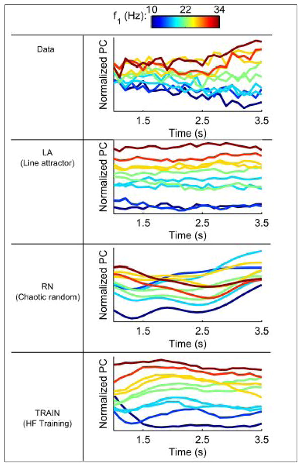
Linear extraction by a modified PCA (Machens et al., 2010) of a time invariant signal that most strongly reflects the coding of stimulus frequency during the delay period. The extraction is done on half the trials, and the projection on the other half. Note that even the random network has a roughly time-invariant component.
A fairly time-independent signal reflecting stimulus frequency can be extracted from all three models. This is particularly surprising for the RN model that has nothing resembling a line attractor in its dynamics. The reason for this is that the stimulus leaves a trace within the network, and it is precisely this trace that the modified PCA method extracts. This analysis should serve as a cautionary note about interpreting results even of an almost assumption free cross-validated population analysis.
Model failures
One prominent feature of the data is not accounted for by any of the models considered in this study. It is an increase in the number of tuned neurons towards the end of the delay period (Figure 6A), indicating an increasingly precise encoding of the stimulus attributes in the population firing rates of the PFC neurons. It has been proposed (Barak et al., 2010; Deco et al., 2010) that these surprising finding could indicate the extraction of information about the stimulus from a synaptic form (selective patterns of short-term synaptic facilitation) into a spiking form. It remains a challenge to future work to develop echo-state random networks and TRAIN networks with short-term synaptic plasticity of recurrent connections.
Figure 6.

Temporal evolution of the fraction of significantly tuned neurons in the data and models. The models were simulated with an identical number of trials as the data to allow evaluation of significance. Note that only the data show an increase in the number of significantly tuned neurons during the delay period.
DISCUSSION
The main goal of this study was to obtain a broader view of the possible mechanisms of working memory, in particular parametric working memory. To this end, we presented a comparative analysis of three network models performing a delayed frequency discrimination of vibrotactile stimuli. By all the measures, it appears fairly clear that the line attractor model (LA) does not adequately describe the experimental data, primarily because neurons in this network all exhibit constant tuning to stimulus features throughout the delay period, whereas many neurons in the data do not (see also Jun et al., 2010). It is noteworthy that a completely random recurrent network that is in the chaotic state (RN) can perform the task reasonably well for delay periods up to about 30 times the time constant of the units, even if the state of the network is not reset before the beginning of each trial. Moreover, some of the neurons in this network retain their tuning to the stimulus until the end of the delay, despite the chaotic dynamics. Overall this network is qualitatively somewhat similar to experimental data. This surprising observation illustrates the difficulty in uncovering the mechanisms of working memory from single neuron recordings and even population analysis of relevant brain regions.
In both the RN and TRAIN networks, which have internal and external noise respectively, the first stimulus is presented at a random time after a random initialization of the network (between 5 and 35 time constants of the network). This means that the network state is different on each trial at the time of the presentation of the first stimulus. In addition, both stimuli (the first and the second) have the same strength, and this is insufficient to put the network into a unique state, independent of its state prior to stimulus onset. If the stimuli were much stronger than this, all memory of the first stimulus would be lost when the second stimulus was presented, making a comparison of them impossible. Thus, these models perform the task at a high level of accuracy despite a large variability in their initial conditions.
Closer analysis indicates that the PFC networks are less random than what is found in the RN model, most prominently, their frequency tuning retains some correlation across the task. This and other features were fairly well captured by the TRAIN model that occupies an intermediate position between the line attractor and RN networks. This network is specifically tuned to the stimuli used in training, and it can retain the tuning to stimulus attributes for significantly longer time than the RN network. Yet in this network as well, many neurons lose their tuning at different epochs of the delay and/or change their tuning properties compared to the stimulus presentation time. This feature is shared by the data.
Although both the RN and TRAIN models start out as randomly connected networks, a distinguishing feature after training is that the connectivity of the RN model is not tuned in any way to the input it receives. Thus, the RN model with appropriately adjusted readouts will perform equivalently for any rearrangement of the stimulus input. The TRAIN model, on the other hand, is adjusted to the specific input it receives during training.
The range of models we considered suggests a possible sequence during learning and development of expertise in the task. It is unlikely that something as organized as the LA model could exist in the neural circuitry of the monkey prior to task learning. Instead, it is more plausible that, initially, the monkey performs the task by extracting whatever signals correlate with reward from existing neural circuitry. At this stage, we argue that the best analogy is with the RN model, not necessarily because the PFC neural circuits are initially random, but because at an early stage they are unlikely to be specialized for the task. With further training, modification of those circuits may occur, leading to something closer to the TRAIN model, and we suggest this approximates the state of the PFC circuitry at the time when the recordings were made. It is possible that with extremely extensive further training, these circuits could become even more organized and develop a true line attractor, as in the LA model. This, in fact, is the trend we observed in the TRAIN model if it was subjected to a more rigorous training procedure, in particular when the delay period was varied from trial to trial. Thus, the different approaches we considered can be viewed as a sequence of models roughly matching stages in the evolution in task performance from novice (RN) to expert (TRAIN) and finally to virtuoso (LA).
METHODS
LA model
This model was described in detail previously (Machens et al., 2005). Briefly, two populations of spiking neurons are connected with self excitation and mutual inhibition (synaptic time constant of 80 msec). The connectivity is tuned such the network implements a line attractor during the delay period. The stimulus tuning during the second stimulus is opposite that during the first, thereby implementing the subtraction operation for stimulus comparison. The model was implemented using the code appearing in the supplementary material of Machens et al., (2005). The only modification was using 17 instead of 500 neurons in each pool to increase the effective noise. We chose to increase noise in this manner because it enabled us to have error trials on all frequency pairs. Another option to decrease overall performance is to impair the tuning of the line attractor, but that would impair only a couple of frequency pairs, unlike the experimental data.
RN model
The RN network is an N-dimensional recurrent neural network defined by
| (1) |
where x is the N-dimensional vector of activations (analogous to the input to a neuron), r is the vector of “firing rates” and the output or readout z is a linear combination of the firing rates. The recurrent feedback in the network is defined by an N×N recurrent weight matrix J with n nonzero elements per row chosen randomly from a Gaussian distribution with mean zero and variance 1/n. The neuronal time constant τ sets the time scale for the model.
Thirty percent of the units received tuned input during the stimuli. Each such unit i, had a random value Bi chosen uniformly between −1 and 1, that determined its tuning. The input ui, is kept at the value zero except when the stimulus is present. Then, it is given by
| (2) |
where f is the stimulus frequency, and h(f) maps the experimental frequency range [10,34] Hz to the range [1,9]. The input ui is always positive (Barak et al., 2010), achieved by adding a bias term to the inputs for which Bi < 0. Thus, h(f) = 1 + 8(f-10)/(34-10) for inputs with B>0, and h(f) = 9 - 8(f-10)/(34-10) for inputs with B<0. In addition, we chose N = 1500, n = 100, g = 1.5 and τ = 100 ms, and ran the model in steps of 0.01τ.
Each trial began with every xi initiated to an independent value from a normal distribution. Following a variable delay of between 500–3500 ms, the first stimulus was applied for 500 ms. For the training only, a variable delay of between 2700–3300 ms was used. During the testing phase, the delay was always 3000ms. The second stimulus followed the delay, and the activity of the network was monitored for a further 500 ms. The firing rate of the network 100 ms after the offset of the second stimulus was collected for 2000 different trials. A linear classifier was trained to discriminate the vectors according to the task, using a maximum margin perceptron (Krauth and Mézard, 1987; Wills and Ninness, 2010).
TRAIN model
The TRAIN network is similar to the RN except for the following differences. The network was smaller, N = 500, n=500. Because connections within the network were modified during training, we could not rely on chaotic dynamics to provide noise, and hence injected white noise to each neuron.
The TRAIN network was trained using the Hessian-Free algorithm for recurrent networks (Martens and Sutskever, 2011). Specifically, the matrix J and weights B and W (Equations 1,2) were trained on the same training trials as described above, but with stimulus amplitudes in the range [0.2,1.8] instead of [1,9]. The model was trained with the HF algorithm in the presence of white noise of amplitude 0.16, and an L2 penalty on the weights, with a weighting coefficient of 2 ×10⁻⁶. The desired output was ±1 for a duration of 100msec, delayed 100msec from the offset of the 2nd stimulus, and error was assessed using mean squared error from the target. After each training iteration (1000 trials), the performance of the model was evaluated on the 10 stimulus conditions. Once the performance exceeded 94%, the noise amplitude was recalibrated to achieve exactly 94% performance, which happened on the 8th iteration with a noise amplitude of 0.2.
Data analysis
Some of the trials in the data were excluded due to suspected spike sorting problems (Barak et al., 2010). To reduce comparison artifacts, for all models the numbers of trials for different stimulus pairs were matched to those of the experimental data. Specifically, model trials were deleted until the number of trials for each stimulus condition matched that of the data.
For all three models, figures 3–6 were generated from simulating the network with 10 trials of each of the 10 stimulus conditions, with a delay of 3000 ms. Figure 2 used 2592 random frequency pairs within the experimental range. For the data and LA model, firing rates of all neurons were calculated for each stimulus condition (f1, f2 pair) in non overlapping 100 ms bins, by averaging the number of spikes emitted by the neuron over all trials with this frequency. Linear tuning was assessed by fitting the function ri(f1,t) = a0(i,t) + a1(i,t) f1. Significance was assessed at the 5% confidence level.
The modified PCA was done as described in Machens et al. (2010), with slight modifications. The time-averaged and frequency-averaged firing rates were defined as rf(i, f) = <ri(f, t)>t and rt(i, f) = <ri(f, t)>f. Three N × N covariance matrices were computed: C computed from r using all stimulus conditions and time bins as samples, Cf computed from rf using all stimulus conditions as samples, and Ct computed from rt using all time bins as samples. The leading eigenvector V of the matrix Cf - Ct was extracted from half the trials, and the activity of the remaining half was projected onto it. Using cross validation, we also computed the total variance explained by this eigenvector, Tr(VTCV )/ Tr(C), and the variance when only stimulus conditions were considered, Tr(VTCf V )/ Tr(Cf ).
Three models are considered for a tactile discrimination task
Models range from highly structure with simple dynamics to random and chaotic
Comparison with data favors an intermediate model
Results suggests a sequence of models applicable at different periods during training
Acknowledgments
O.B. was supported by DARPA grant SyNAPSE HR0011-09-C-0002. D.S. and L.A. were supported by NIH grant MH093338. The research of R.R. was partially supported by an international Research Scholars Award from the Howard Hughes Medical Institute and grants from CONACYT and DGAPA-UNAM. M.T. is supported by the Israeli Science Foundation. We also thank the Swartz, Gatsby, Mathers and Kavli Foundations for continued support.
Glossary
- PFC
prefrontal cortex
- LA
line attractor model
- RN
random network model
- TRAIN
trained network model
Footnotes
Publisher's Disclaimer: This is a PDF file of an unedited manuscript that has been accepted for publication. As a service to our customers we are providing this early version of the manuscript. The manuscript will undergo copyediting, typesetting, and review of the resulting proof before it is published in its final citable form. Please note that during the production process errors may be discovered which could affect the content, and all legal disclaimers that apply to the journal pertain.
References
- Amit DJ, Brunel N. Model of global spontaneous activity and local structured activity during delay periods in the cerebral cortex. Cereb Cortex. 1997;7:237–252. doi: 10.1093/cercor/7.3.237. [DOI] [PubMed] [Google Scholar]
- BADDELEY A, Hitch G. Working Memory. In: Bower G, editor. Recent Advances in Learning and Motivation. New York: Academic Press; 1974. pp. 47–90. [Google Scholar]
- Barak O, Tsodyks M, Romo R. Neuronal population coding of parametric working memory. Journal of Neuroscience. 2010;30:9424. doi: 10.1523/JNEUROSCI.1875-10.2010. [DOI] [PMC free article] [PubMed] [Google Scholar]
- Ben-Yishai R, Bar-Or RL, Sompolinsky H. Theory of orientation tuning in visual cortex. Proceedings of the National Academy of Sciences. 1995;92:3844–3848. doi: 10.1073/pnas.92.9.3844. [DOI] [PMC free article] [PubMed] [Google Scholar]
- Brody CD, Hernandez A, Zainos A, Romo R. Timing and neural encoding of somatosensory parametric working memory in macaque prefrontal cortex. Cerebral Cortex. 2003;13:1196–1207. doi: 10.1093/cercor/bhg100. [DOI] [PubMed] [Google Scholar]
- Deco G, Rolls ET, Romo R. Synaptic dynamics and decision making. Proceedings of the National Academy of Sciences. 2010;107:7545–7549. doi: 10.1073/pnas.1002333107. [DOI] [PMC free article] [PubMed] [Google Scholar]
- Funahashi S, Bruce CJ, Goldman-Rakic PS. Mnemonic coding of visual space in the monkey’s dorsolateral prefrontal cortex. J Neurophysiol. 1989;61:331–349. doi: 10.1152/jn.1989.61.2.331. [DOI] [PubMed] [Google Scholar]
- Funahashi S, Bruce CJ, Goldman-Rakic PS. Visuospatial coding in primate prefrontal neurons revealed by oculomotor paradigms. J Neurophysiol. 1990;63:814–831. doi: 10.1152/jn.1990.63.4.814. [DOI] [PubMed] [Google Scholar]
- Fuster JM, Alexander GE. Neuron activity related to short-term memory. Science. 1971;173:652–654. doi: 10.1126/science.173.3997.652. [DOI] [PubMed] [Google Scholar]
- Hebb DO. The organization of behavior: a neuropsychological theory (Wiley) 1949 [Google Scholar]
- Hopfield JJ. Neural networks and physical systems with emergent collective computational abilities. Proceedings of the National Academy of Sciences. 1982;79:2554. doi: 10.1073/pnas.79.8.2554. [DOI] [PMC free article] [PubMed] [Google Scholar]
- Jaeger H. The“ echo state” approach to analysing and training recurrent neural networks-with an erratum note’ (Technical Report GMD Report 148, German National Research Center for Information Technology) 2001 [Google Scholar]
- Joshi P. From memory-based decisions to decision-based movements: A model of interval discrimination followed by action selection. Neural Networks. 2007;20:298–311. doi: 10.1016/j.neunet.2007.04.015. [DOI] [PubMed] [Google Scholar]
- Jun JK, Miller P, Hernández A, Zainos A, Lemus L, Brody CD, Romo R. Heterogenous population coding of a short-term memory and decision task. J Neurosci. 2010;30:916–929. doi: 10.1523/JNEUROSCI.2062-09.2010. [DOI] [PMC free article] [PubMed] [Google Scholar]
- Krauth W, Mézard M. Learning algorithms with optimal stability in neural networks. Journal of Physics A: Mathematical and General. 1987;20:L745. [Google Scholar]
- Maass W, Natschläger T, Markram H. Real-time computing without stable states: A new framework for neural computation based on perturbations. Neural Computation. 2002;14:2531–2560. doi: 10.1162/089976602760407955. [DOI] [PubMed] [Google Scholar]
- Machens CK, Romo R, Brody CD. Flexible control of mutual inhibition: a neural model of two-interval discrimination. Science. 2005;307:1121–1124. doi: 10.1126/science.1104171. [DOI] [PubMed] [Google Scholar]
- Machens CK, Romo R, Brody CD. Functional, But Not Anatomical, Separation of “What” and “When” in Prefrontal Cortex. J Neurosci. 2010;30:350–360. doi: 10.1523/JNEUROSCI.3276-09.2010. [DOI] [PMC free article] [PubMed] [Google Scholar]
- Martens J, Sutskever I. Learning recurrent neural networks with Hessian-free optimization. Proc. 28th Int. Conf. on Machine Learning; Bellevue, WA. 2011. [Google Scholar]
- Miller P, Brody CD, Romo R, Wang XJ. A recurrent network model of somatosensory parametric working memory in the prefrontal cortex. Cerebral Cortex. 2003;13:1208–1218. doi: 10.1093/cercor/bhg101. [DOI] [PMC free article] [PubMed] [Google Scholar]
- Miller P, Wang XJ. Inhibitory control by an integral feedback signal in prefrontal cortex: A model of discrimination between sequential stimuli. Proceedings of the National Academy of Sciences. 2006;103:201–206. doi: 10.1073/pnas.0508072103. [DOI] [PMC free article] [PubMed] [Google Scholar]
- Miyashita Y, Chang HS. Neuronal correlate of pictorial short-term memory in the primate temporal cortex. Nature. 1988;331:68–70. doi: 10.1038/331068a0. [DOI] [PubMed] [Google Scholar]
- Rajan K, Abbott LF, Sompolinsky H. Stimulus-dependent suppression of chaos in recurrent neural networks. Phys Rev E. 2010;82:011903. doi: 10.1103/PhysRevE.82.011903. [DOI] [PMC free article] [PubMed] [Google Scholar]
- Romo R, Brody CD, Hernandez A, Lemus L. Neuronal correlates of parametric working memory in the prefrontal cortex. Nature. 1999;399:470–473. doi: 10.1038/20939. [DOI] [PubMed] [Google Scholar]
- Romo R, Hernández A, Zainos A, Lemus L, Brody CD. Neuronal correlates of decision-making in secondary somatosensory cortex. Nat Neurosci. 2002;5:1217–1225. doi: 10.1038/nn950. [DOI] [PubMed] [Google Scholar]
- Romo R, Salinas E. Flutter discrimination: neural codes, perception, memory and decision making. Nature Reviews Neuroscience. 2003;4:203–218. doi: 10.1038/nrn1058. [DOI] [PubMed] [Google Scholar]
- Seung HS. Proceedings of the 1997 Conference on Advances in Neural Information Processing Systems 10. Cambridge, MA, USA: MIT Press; 1998. Learning continuous attractors in recurrent networks; pp. 654–660. [Google Scholar]
- Shafi M, Zhou Y, Quintana J, Chow C, Fuster J, Bodner M. Variability in neuronal activity in primate cortex during working memory tasks. Neuroscience. 2007;146:1082–1108. doi: 10.1016/j.neuroscience.2006.12.072. [DOI] [PubMed] [Google Scholar]
- Singh R, Eliasmith C. Higher-dimensional neurons explain the tuning and dynamics of working memory cells. Journal of Neuroscience. 2006;26:3667–3678. doi: 10.1523/JNEUROSCI.4864-05.2006. [DOI] [PMC free article] [PubMed] [Google Scholar]
- Sompolinsky H, Crisanti A, Sommers HJ. Chaos in Random Neural Networks. Phys Rev Lett. 1988;61:259–262. doi: 10.1103/PhysRevLett.61.259. [DOI] [PubMed] [Google Scholar]
- Sussillo D, Abbott LF. Generating coherent patterns of activity from chaotic neural networks. Neuron. 2009;63:544–557. doi: 10.1016/j.neuron.2009.07.018. [DOI] [PMC free article] [PubMed] [Google Scholar]
- Wang XJ. Synaptic reverberation underlying mnemonic persistent activity. Trends Neurosci. 2001;24:455–463. doi: 10.1016/s0166-2236(00)01868-3. [DOI] [PubMed] [Google Scholar]
- Wang XJ. Decision making in recurrent neuronal circuits. Neuron. 2008;60:215. doi: 10.1016/j.neuron.2008.09.034. [DOI] [PMC free article] [PubMed] [Google Scholar]
- Wang X-J. Attractor Network Models. In: Squire Larry R., editor. Encyclopedia of Neuroscience. Oxford: Academic Press; 2009. pp. 667–679. [Google Scholar]
- Wills AG, Ninness B. QPC - Quadratic Programming in C 2010 [Google Scholar]