Derivation of Fixed Partial Charges for Amino Acids Accommodating a Specific Water Model and Implicit Polarization

Abstract

We have developed the IPolQ method for fitting non-polarizable point charges to implicitly represent the energy of polarization for systems in pure water. The method involves iterative cycles of molecular dynamics simulations to estimate the water charge density around the solute of interest followed by quantum mechanical calculations at the MP2/cc-pV(T+d)Z level to determine updated solute charges. Lennard-Jones parameters are updated starting from the Amber FF99SB nonbonded parameter set to accommodate the new charge model, guided by the comparisons to experimental hydration free energies (HFEs) of neutral amino acid side chain analogs and assumptions about the computed HFEs for charged side chains. These Lennard-Jones parameter adjustments for side chain analogs are assumed to be transferable to amino acids generally, and new charges for all standard amino acids are then derived in the presence of water modeled by TIP4P-Ew. Overall, the new charges depict substantially more polarized amino acids, particularly in the backbone moieties, than previous Amber charge sets. Efforts to complete a new force field with appropriate torsion parameters for this charge model are underway. The IPolQ method is general, applicable to arbitrary solutes.

2 Introduction

For the approximately thirty year history of bimolecular simulations, models of protein and nucleic acid systems have focused on a representation of individual atoms as separate beads, connected by a harmonic or other simple bonding potential, drawn together by isotropic coulomb and dispersion interactions between sites located on the nuclei, and held against collapse by rapidly divergent repulsive functions also centered at the nuclei. In its simplest form, this framework neglects polarization,¹ charge penetration,² resonance, and charge transfer effects,³ though numerous approaches have been offered to approximate these phenomena in the context of a classical mechanics model.

Effective potentials for water developed in the 1980s^4,5 remain in use today with only minor modifications.⁶ Multiple lineages of protein and nucleic acid force fields begun in the 1990s,^7,8 as well as rigorous algorithms for handling long-ranged electrostatics,⁹ likewise remain essential components of modern simulations. Algorithms for propagating particle dynamics in parallel,^10,11 combined with a giant increase in computer processor speeds and integrated core designs, have put these models to the test in the past decade by enabling researchers to measure their consequences over simulations reaching biological time scales.^12,13 Keeping the perspective that these models are attempts to emulate quantum mechanical systems with vastly simplified classical interactions, they have achieved impressive results.¹⁴ However, numerous deficiencies have also been identified;¹⁵ also of significant concern is that the various solvent and bimolecular models were often not derived in conjunction with one another and have therefore been prone to questions over which combinations, if any, are truly appropriate.¹⁶ The era of simple point charge models, at least as the engine of long-timescale biomolecular simulations, is drawing to a conclusion: a synthesis of the products of this era, including accurate models of neat water, long-ranged electrostatics, solvent polarization, and thermodynamic calculations, is an opportunity to assess progress as more complex classical models come into service.

In this article we present a new derivation of atomic partial charges which integrates a theoretical framework with solvent polarization implied by the presence of a field of background charges included in quantum mechanical calculations for Restrained Electrostatic Potential (REsP) fitting.¹⁷ Other approaches along this line have been explored;¹⁸ our method, termed IPolQ for “Implictly Polarized Charges,” is a direct alternative to partial charges found in the existing Cornell⁸ and Duan¹⁹ charge sets in existing AMBER force fields. Our exact method for fitting the partial charges retains the spirit of the original Kollmann REsP, but fits the quantum mechanical electrostatic potential obtained from MP2/cc-pV(T+d)Z calculations over a broad solvent-accessible region surrounding each molecule, covering roughly the first three solvent layers. IPolQ specifically incorporates the TIP4P-Ew water model,²⁰ which gives strong reproduction of water’s liquid properties at the temperatures and pressures relevant to biology. The TIP4P water geometry has also been reported to be the best of the TIP models for maintaining water:water radial distribution functions in QM/MM simulations similar to the methods used in this study.²¹

In order to improve hydration free energies of side chain analogs modeled by IPolQ, Lennard-Jones terms on critical atoms were also recalibrated. These modifications for the side chain analogs are assumed to be transferable to larger polypeptides. By construction, the combination of the new charge protocol and adjustments to Lennard-Jones parameters offers improved estimates of the hydration free energies of amino acid side chain analogs relative to the Cornell charge set and its derivatives. Also, by examining the errors in the electrostatic potential that our fitted charges make in attempting to reproduce the quantum mechanical target, we find that the inaccuracies arising from locating non-polarizable charges on nuclei may be of greater magnitude than the differences between either of the previous Amber charge sets and IPolQ. We show that the electrostatic characteristics near the surfaces of molecules are more affected by the locations of fitted charge centers (the nuclear-only treatment being nearly universal in biomolecular force fields), while the long-ranged dipoles are dependent on the choice of quantum mechanical fitting target.

Of greater interest is whether IPolQ will lead to different protein hydration characteristics. As a consequence of the new quantum mechanical target model, the polarities of side chain amides are increased while certain side chain hydroxyl groups tend to be decreased relative to their Cornell or Duan counterparts. When applied to amino acid dipeptides, the dipoles of the backbone carbonyl and amide groups are increased, suggesting that proteins modeled with IPolQ may behave differently in water than proteins modeled with the either the Cornell or Duan charge sets. As it stands, the new charge set is ready for incorporation into a new force field, but it will require a refit of dihedral terms before this force field is complete.

3 Methods

When deriving parameters for non-polarizable force fields with the Restrained Electrostatic Potential (REsP) method, the principal assumption is that the electrostatic properties of a molecular system are best determined by mimicking the electrostatic potential outside the molecular surface as found in a suitable quantum mechanical calculation. Because instantaneous polarization of the system by neighboring molecules cannot be captured except in an average sense, the quantum mechanical calculation should, if possible, reflect this average. One approach for estimating the mean polarization effect, for a given condensed-phase environment, has been given by Karamertzanis and colleagues.²² We apply this approach to generate electrostatic potentials for amino acid dipeptides and fit a set of molecular mechanics charges, along with a refined procedure for selecting sites throughout the solvent-accessible region surrounding each dipeptide. The resulting protocol for fitting charges is an iterative application of classical molecular dynamics simulations that generate average solvent charge densities around the molecules of interest and quantum mechanical calculations at the level of Møller-Plesset second order perturbation (MP2) theory.

While REsP fitting is appealing because it produces a deterministic set of charges given a sufficiently large data set and a defined set of constraints, the charge set is malleable if different constraints are applied to the fit and ultimately there is no way to validate the charges in terms of experimental observables. We therefore chose to incorporate known hydration free energies (HFEs) of amino acid side chain analogs into the fitting procedure by adjusting Lennard-Jones parameters.

3.1 Derivation of partial charges for a non-polarizable model of the condensed phase

In the approach of Karamertzanis, et al.,²² one considers three possible polarization states for a molecule. The first is an unpolarized state that exists in vacuum. The second is a time or ensemble-averaged polarization state that exists in a condensed phase environment: the molecule imparts structure to the surrounding medium, and the medium in turn creates an electrostatic reaction field which polarizes the molecule. The third state is the arithmetic average of the previous two. A fixed charge force field may represent the energy penalty of electronic polarization either by a post hoc correction term^23,24,5 or by weakening the interaction between static monopoles or dipoles to implictly account for the polarization energy as part of the atomic interactions. Alternatives for weakening these interactions have been proposed;²⁵ Karamertzanis and colleagues begin with assumptions that lead to a formal account of the induction energy penalty by averaging of vacuum and condensed-phase polarities.

The electrostatic energy of a system of fixed dipoles can be written:

$$U=\frac{1}{2}\sum _i-{\mathit{\mu }}_i\mathbf{E}({\mathbf{r}}_i)=\frac{1}{2}\sum _{i>j}{\mathit{\mu }}_i{\mathbf{T}}_{ij}{\mathit{\mu }}_j$$ (1)

where E(r_i) is the electric field at the site of dipole i. The tensor T_ij is constructed from the identity tensor I, the tensor product of unit vectors r̂_ij pointing between the dipoles, and the displacement r_ij separating the dipoles:

$${\mathbf{T}}_{ij}=\frac{\mathbf{I}-3{\widehat{r}}_{ij}{\widehat{r}}_{ij}}{{\mid {\mathbf{r}}_{ij}\mid }^3}$$ (2)

The electric field at site i is in turn given by:

$$\mathbf{E}({\mathbf{r}}_i)=\sum _{j\ne i}-{\mathbf{T}}_{ij}{\mathit{\mu }}_j$$ (3)

In a point charge representation of the electrostatics, the electric field is actually computed in the sum over all pairs of point charges.

To summarize Karamertzanis’s argument, we consider a polarizable system whose molecules have a gas-phase dipole moment of μ₀. These molecules are placed in a field E(r) which causes them to polarize to some extent, producing a new dipole moment μ= μ₀ + Δμ. The energy of this system can be written:

$$U=\sum _i\frac{[\mathrm{\Delta }{\mathit{\mu }}_i{\mathit{\alpha }}_i^{-1}\mathrm{\Delta }{\mathit{\mu }}_i]}{2}-\sum _i\left({\mathit{\mu }}_{0,i}+\mathrm{\Delta }{\mathit{\mu }}_i\right)\mathbf{E}({\mathbf{r}}_i)$$ (4)

where α is the molecular polarizability tensor. The first term (the polarization energy) is always positive, grows with increasing polarization, and repels any molecule from the source of the field. The second term is the interaction of the net dipole of molecule i with the field. If Δμ_i, the polarization of site i, runs parallel to the field, this reduces the energy of the system and attracts it to the source of the field. The total polarization of molecules throughout the system will adjust to minimize the sum of both terms. Computing dU/dΔμ and setting this derivative to zero results in the familiar expression relating the degree of polarization to the field strength and intrinsic polarizability:

$$\mathrm{\Delta }{\mathit{\mu }}_i={\mathit{\alpha }}_i\mathbf{E}({\mathbf{r}}_i)$$ (5)

In a polarizable force field or a quantum model, the charge density will satisfy this condition. Whenever it is true, the above expression may be inserted into the polarization cost to produce:

$$U=\sum _i\frac{[\mathrm{\Delta }{\mathit{\mu }}_i{\mathit{\alpha }}_i^{-1}{\mathit{\alpha }}_i\mathbf{E}({\mathbf{r}}_i)]}{2}-\sum _i\left({\mathit{\mu }}_{0,i}+\mathrm{\Delta }{\mathit{\mu }}_i\right)\mathbf{E}({\mathbf{r}}_i)=-\sum _i\left({\mathit{\mu }}_{0,i}+\frac{\mathrm{\Delta }{\mathit{\mu }}_i}{2}\mathbf{E}({\mathbf{r}}_i)\right)$$ (6)

This can be viewed as the energy required to place a non-polarizable dipole of μ = μ₀ + Δμ/2 into the field E. Therefore, if the appropriate degree of polarization Δμ can be computed, it is possible to use a fixed-charge representation if the molecules of the system are set to have dipoles halfway between their isolated states and those they would explicitly take on in the presence of the field. As we show with three simplified systems in the Supporting Information, the modification of the charges on each molecule implicitly accounts for the polarization energy cost: to a first approximation, the energy penalty is spread throughout the interacting pairs of atoms.

3.2 Representing charge polarization in a fixed-charge model: IPolQ

From the preceding derivation, the goal is to determine an appropriate reaction field to represent the electrostatic effects of a condensed phase environment on a molecule of interest. Then, two sets of charges are determined: one appropriate to represent the fully polarized state of the molecule in the reaction field, and another to represent the unpolarized state of the molecule in vacuum. The Implicitly Polarized Charge (IPolQ) scheme takes the average of these two sets to represent electronic polarization of the molecule in the condensed phase within the confines of a non-polarizable model. For application to proteins and other biomolecules, the condensed phase is liquid water.

Because the solute itself influences the surrounding hydration structure and thus the solvent reaction field potential, the challenge with the IPolQ method is to represent the solvent reaction field in a self-consistent manner with the parameters on that solute. The work cycle illustrated in Figure 1 shows how this self-consistency is achieved through an iterative process of molecular mechanics simulations, quantum calculations, and data fitting. The remaining sections of the Methods give details on each step of cycle (1), and also the thermodynamic integration that guided parameter adjustments in cycle (2).

Figure 1. Work cycle for the Implicitly Polarized Charges (IPolQ) method.

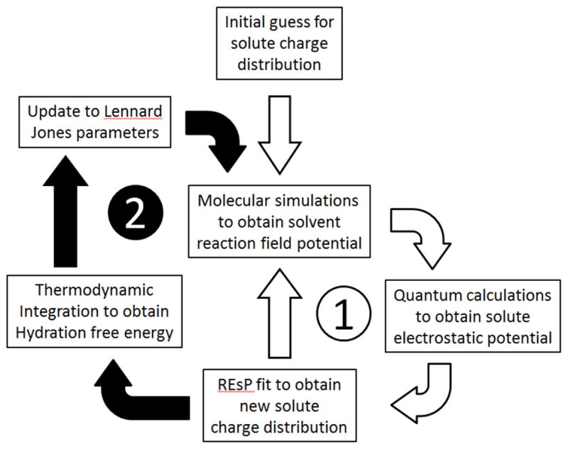
Starting from any reasonable guess as to the initial solute charge distribution, the IPolQ method iteratively computes a solvent reaction field potential with molecular mechanics simulations, then a solute electrostatic potential via quantum calculations, and applies a linear least squares fit to obtain a new molecular mechanics charge distribution on the solute. Subcycle (1) is iterated until the fitted solute charges converge. Lennard-Jones σ were adjusted to optimize the hydration free energies of some molecules, which in turn influences the solvent reaction field potential. A pass through cycle (2) implies additional iterations of cycle (1).

3.3 Amino acid fragments and their hydration free energies

New charge sets obtained by iterations of cycle (1) in Figure 1 are not necessarily compatible with the Lennard-Jones parameters from the existing AMBER force fields. As a first-order correction, we computed charges for amino acid side-chain analogs by cycle (1), then adjusted Lennard-Jones parameters by cycle (2) and continued to iterate cycle (1) to bring the hydration free energies (HFEs) of the side chain analogs into agreement with experiment. We restricted ourselves to adjusting the σ parameters of the Lennard-Jones function:

$$U_{ij}=4\epsilon \left[{\left(\frac{{\sigma }_{ij}}{{\mathbf{r}}_{ij}}\right)}^{12}-{\left(\frac{{\sigma }_{ij}}{{\mathbf{r}}_{ij}}\right)}^6\right]$$ (7)

where σ_ij is derived by the Lorentz-Berthelot combining rules. These modifications were assumed to be transferable to amino acids in proteins.

Hydration free energies were computed using thermodynamic integration where solute-solvent interactions were decoupled using a soft-core treament for the repulsive components as implemented in the AMBER molecular dynamics package.²⁶ Following the procedures of a previous study,²⁷ we placed neutral solutes in baths of water molecules sufficient to immerse them with at least 12Å separating the solute from the boundary of the equilibrated simulation box (for ionic species, this was increased to 20 Å). After 500ps of dynamics in the NPT ensemble to equilibrate the system, thermodynamic integration was performed to evaluate free energies in twelve windows with Gaussian quadrature integration of the form:

$$\mathrm{\Delta }A=\sum _i{w}_i{\langle \frac{\delta U}{\delta \lambda }\rangle }_i$$ (8)

Dynamics in each window were propagated for 5ns. All simulations were performed at 300K, with Smooth Particle-Mesh Ewald⁹ periodic electrostatics, a 10Å cutoff and long-ranged tail correction for Lennard-Jones interactions, and a 1fs time step. Uncertainty in the TI results was estimated by repeating the runs in each window for an additional 5ns; the uncertainties in the calculated HFEs of all solutes were less than 0.2 kcal/mol.

To compute hydration free energies for ionic species requires additional assumptions. We follow the ideas and thermodynamic cycle given by Pearson²⁸, compiled in recently published work,²⁹ and summarized with relevance to this study in Figure 2. Values pertaining to each ionic amino acid for each step of the thermodynamic cycle are given in Table 6; it is important to note that the cycle contains processes whose energies are uncertain. For instance, Pearson’s estimate of acetate’s HFE, −75 kcal/mol, is updated to −89 kcal/mol by taking the intrinsic basicity of acetic acid to be 341.5^30,31,32 rather than 336.5 kcal/mol, the HFE of non-ionized acetic acid to be −6.7³³ rather than −4.8 kcal/mol, and the HFE of the proton to be −252.5³⁴ rather than −259.5; all of these choices make the target HFE of acetate, the value which should emerge from thermodynamic integration, appear more favorable.

Figure 2. Thermodynamic cycle for calculation of hydration free energies (HFEs) of acids, based on the ideas of Pearson.²⁸.

“(B)” may be substituted for “A-” if conjugate acids are to be analyzed. White arrows denote processes whose values must be taken as given, but are uncertain (and subject to revision). Orange and gray arrows correspond to processes whose free energies are calculated from simulations. The lone blue arrow is an experimentally observable process. [1] is the intrinsic / gas-phase basicity. [2] represents a change in the standard concentration from one atmosphere to the 1 molar concentration used in liquid state measurements; it is assumed to be the same for all species. [3] and [4] are polarization energies required to convert the gas phase charge distribution of species (A-) to the charge distribution used in the force field, which is intended to model the electron density of aqueous (A-). The polarized (A-) is indicated by a dotted ring around its icon. [5] and [6] correspond to simulation results for HFEs of fixed-charge models, as described in the text. [7] is the hydration free energy of the proton, the exact value of which is uncertain. [8] is the actual hydration free energy taken from pK_a measurements of the species (AH) in water. Note that the combination of [3] and [5], or [4] and [6], corresponds to the hydration affinity as measured by Wolfenden for neutral species, or as estimated in Table 2 for charged species, and to the ideal result of a thermodynamic integration calculation performed with a force field incorporating a polarization energy correction.

Specific changes to Lennard-Jones parameters and the motivation for each change are given in the Results.

3.4 Quantum mechanical calculations

The quantum mechanical calculation standard for all molecules in both isolated and solvated states was chosen to be MP2 calculations with the cc-pV(T+d)Z basis set.^35,36,37,38 The level of theory and basis set were selected to be sufficiently accurate for computation of molecular multipole moments and electrostatic potentials; in addition, this level of theory matches that used for computation of potential energy surfaces in previous optimizations of molecular mechanics torsion potentials.³⁹ The Gaussian09 software package (Gaussian, Inc., Wallingford CT) was used for all quantum calculations.

3.5 Derivation of solvent reaction field for REsP fitting

Having selected the approach for abstracting a meaningful set of charges from quantum electrostatics and the type of quantum mechanical calculation to perform, the methods for generating conformations of the molecules of interest, and solvent environments around each of those conformations, remain to be addressed. The condensed-phase environment was chosen to be the solvent with which we intend the resulting force field to be applied: a bath of TIP4P-Ew water.²⁰ Molecular dynamics simulations for generating molecular conformations and solvent distributions were performed in a similar manner to the TI protocol described above, but with a 2fs time step. High-temperature dynamics of each dipeptide or side chain analog were performed at 450K for 10ns. Snapshots were collected every 500ps for use as seeds to generate average solvent configurations for each conformation, as shown for the case of arginine dipeptide in Figure 3. In order to generate an average solvent density around each solute conformation, the snapshots extracted from the high-temperature dynamics were first energy-minimized with 10.0 kcal/mol-Ų positional restraints on all heavy atoms. All atoms of the solute were then completely frozen in place as water molecules sampled configurations around their surfaces, as illustrated in Figure 4. Simulations of the frozen solutes were performed in the constant volume ensemble at 298K over 500ps; 200 snapshots were collected at 2ps intervals following 100ps of discarded dynamics. The locations of water molecules in these snapshots served to create a field of point charges surrounding the molecules of interest for subsequent MP2/cc-pV(T+d)Z calculations.

Figure 3. Conformations of the arginine dipeptide used for charge refinement.

The arginine side chain explores all three χ₁ rotamer states, and the backbone takes on a variety of Φ and Ψ angles. Although we did not attempt to select conformations to precisely match known PDB distributions or a Ramachandran plot, we feel that the most important aspect of the fitting set is that it comprise a variety of conformations. As shown in Figure 5 of the main text, the REsP fit implies many compromises in the electrostatic propreties influencing the first solvent layer. The best way to minimize the chance that these compromises will superimpose to create regions of large error is to make the fitting set comprehensive.

Figure 4. Time-averaged water distributions around each dipeptide conformation indicate the solvent charge density.

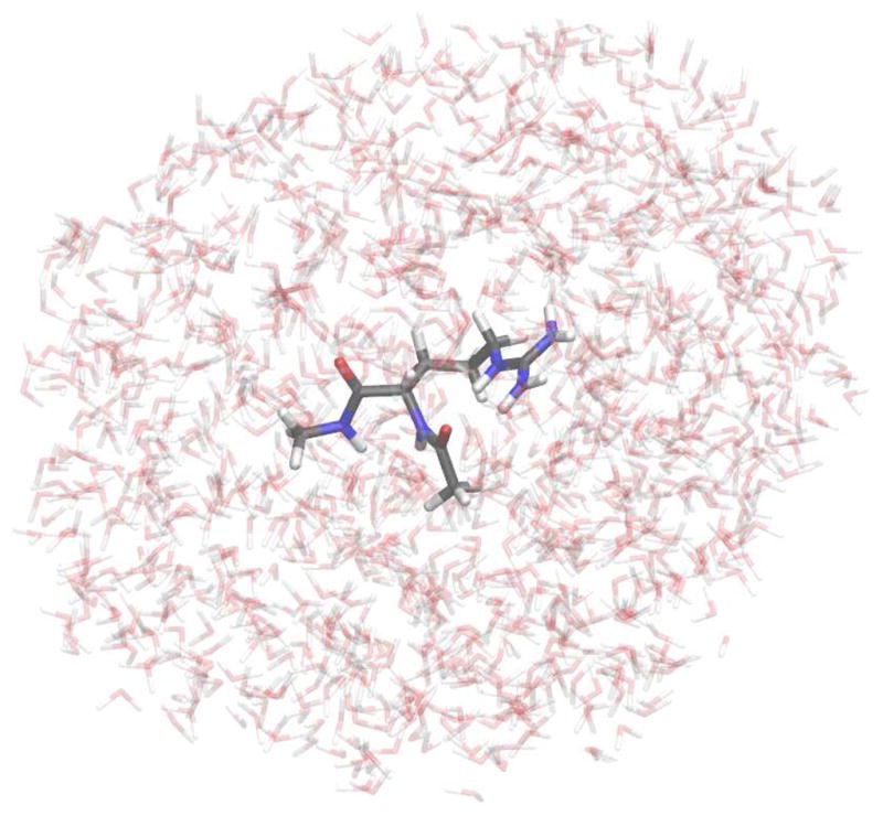
The partial atomic charges of water molecules moving about the solute produce a solvent charge distribution which can then be superimposed on quantum calculations.

We sought to reproduce the electrostatic field due to infinite, periodic electrostatics within the confines of the isolated system on which the MP2 calculation was performed. All solvent molecules whose centers of mass resided within 10Å of the solute were included in the MP2 calculation; other waters were discarded. It was necessary to compute a solvent reaction field that, at the sites of solute atoms, had converged in two respects: with respect to the number of simulation snapshots included in the average, and with respect to the subset of water surrounding the solute included in each solvent configuration. We verified that the first criterion had been met by averaging over snapshots from 4ns, as opposed to 400ps, simulations. The second criterion is more complicated to assess, but we assumed we had a large enough simulation cell and took the electrostatic field due to all solvent particles in that periodic cell to be the standard. For neutral solutes, it was sufficient to include just the subset of water molecules mentioned above. However, in case of ionic amino acid dipeptides, the solvent contained counterions and it was not sufficient to simply include only particles within the 10Å shell around the solute. In these cases, a shell of additional point charges, approximately one charge per 12Ų on a shell 10Å from any solute atom, was introduced into the MP2 calculations. This approximated the influence of solvent present in the molecular dynamics simulation beyond the 10Å cutoff, as illustrated in Figure 5. The shell charges were fitted with a procedure very similar to the REsP optimization of the solute charges described below. With hundreds of charges to place and only the components of the electrostatic field at the solute atom sites as a guide, this would be an underdetermined problem. However, we applied harmonic restraints to hold each shell charge to a small value, typically less than one tenth of an electron’s charge. In this manner, the system of equations becomes slightly over-determined and the field generated by these shell charges is smooth in the vicinity of the solute.

Figure 5. Corrections for infinite electrostatics in non-periodic quantum calculations.

For ionic amino acids, the charge distribution in Figure 4 is not an adequate approximation of the solvent reaction field. To overcome this, we computed the electrostatic field due to all solvent particles in the molecular mechanics simulation, including counterions. This information was used to fit a set of boundary charges to complement the charge distribution of solvent particles near the solute. In the figure above, the effects due to water molecules which are faded out on the right hand panel are represented by the blue and green boundary charges.

The charge distribution was determined by TIP4P-Ew configurations and parameters, but with one final modification. The TIP4P-Ew model itself can be viewed as a consequence of Karamertzanis’s arguments: it is perhaps not a coincidence that nearly all fixed-charge water models carry dipoles of roughly 2.3D, halfway between the gas-phase water dipole of 1.85D and the measured solution-phase dipole of 2.6D to 2.9D.⁴⁰ In the framework we have chosen, it is appropriate to compute the electrostatic field due to charges of fully polarized water, and insert this field into quantum calculations, before averaging the fitted solute charges. We placed charges of −0.6295 × 10⁻² electron charge units and +0.31475 × 10⁻² electron charge units at the locations of TIP4P-Ew extra points and TIP4P-Ew hydrogen atoms in the 200 snapshots taken from our simulations. These are 1/200th of the charges of a polarized version of TIP4P-Ew, possessing a dipole greater than normal TIP4P-Ew by the same degree that TIP4P-Ew exceeds the dipole of water vapor.

3.6 Details of REsP fitting: Sites, constraints, and variables

Fitting sites for the REsP method were selected in a manner that is complicated to describe but intuitively sensible: the goal was to select points that evenly sampled the solvent-accessible region around each solute conformation (including the region which might be accessible to polar hydrogens on water molecules or other polar groups on nearby molecules). Grids of evenly spaced points were generated with the Gaussian09 cubegen utility; fitting points were selected such that all fitting points were accessible to the oxygen or hydrogen atoms of a TIP4P-Ew solvent probe pressed against the solute with less than 2 kcal/mol Lennard-Jones energy penalty. All points within 3Å of the solute surface and at least 0.4Å from one another were selected; beyond 3Å from the solute surface, points that satisfied the mutual distance constraints were randomly selected with decreasing likelihood according to their distance from the solute until a maximum of 5,000 fitting points per solute conformation had been selected. In this manner, fitting points were dispersed evenly throughout the first solvent shell and balanced with fitting points in the second shell.

When fitting charges for amino acids, we chose blocked dipeptides (Acetyl–Amino Acid–N-methyl Acetamide) as model systems, omitting one of the blocking groups to fit charges for N- or C-terminal residues. Five types of constraints were imposed on the fit in order to make the results useful for protein simulations. First, we followed a convention of the Cornell charge set and collected the backbone nitrogen, peptide hydrogen, oxygen, and carbonyl carbon atoms in N-terminal, non-terminal, and C-terminal amino acids into grouped variables in the REsP fit rather than letting each instance of every backbone atom take on a different charge as was done in the Duan charge refit.¹⁹ This uniformity of backbone charges facilitates the development of a common set of dihedral parameters (as will be discussed in the following section) by reducing the variability of electrostatic interactions between adjacent atoms. Second, because we are interested in fitting parameters for residues of biological heteropolymers, we assumed that the charges of any residue or blocking group would be insensitive to the identities of adjacent residues in any chains. Third, as is customary in REsP fits, the charges of equivalent, symmetry-related atoms such as the alanine methyl group hydrogens were grouped into single variables. Fourth, in order to prevent methyl carbons or other buried atoms from taking on spurious, large charges, the charges on methyl carbon atoms with no polar groups were harmonically restrained towards zero. Finally, the charges of each amino acid or blocking group were required to sum to an integer value depending on the protonation state. Following the arguments of Karamertzanis and colleagues, the resulting sets of charges are the proper non-polarizable point-charge representations of the electrostatics of hydrated amino acids.

4 Results

4.1 Hydration free energies of amino acid side chain and backbone analogs

The first, and most challenging, part of this study was the modeling of amino acid side chain analogs and calculations of their hydration free energies (HFEs). The results are shown in Figures 6 and Figure 7, and listed in Tables 2 and 3 of the Supporting Information. We compare our derived charges to the Cornell charges in the context of the Amber FF99 force field.⁴¹ Preserving all FF99 Lennard-Jones parameters, our charge scheme produces models with slightly lower accuracy in their HFE predictions; it should be noted that FF99 itself was not designed specifically to reproduce experimental HFEs. We adjusted Lennard-Jones σ parameters to bring some of the computed HFEs into closer agreement with experiment, as enumerated in Table 6. First, the radii of hydroxyl oxygen and thiol sulfur atoms were reduced to make the HFEs of these groups more favorable. This optimization was guided by methanol and ethanol, as para-cresol (Tyr side chain) was also disfavorably hydrated according to our charge scheme but its phenyl group may have consequences for hydration that we cannot capture in this force field. We also increased the nitrogen radii of side chain (primary) amides and the oxygen radii of all amides (including backbone secondary amides) to disfavor hydration of these groups. The hydration free energies of charged side chain analogs were in need of the largest corrections, but also have the largest experimental HFEs. Carboxylate oxygen radii were increased by 12% and terminal amine radii (as found on Lys side chains and peptide N-termini) were decreased by 8%. By incorporating these changes, the mean unsigned error of computed HFEs for neutral side chain analogs was reduced from 1.55 kcal/mol to 0.63 kcal/mol; the mean unsigned error of charged side chain analogs was reduced from 9.79 to 4.84 kcal/mol. While further improvement may be possible, it would require adjustment of many more Lennard-Jones parameters based on scarce experimental data, with uncertainty in the transferability of the results. The complete tables of partial charges for side chain analogs may be found in the Supporing Information.

Figure 6. Comparison of estimated HFEs for uncharged side chain analogs.

The HFEs for polar and nonpolar side chain analogs are estimated in TIP3P and TIP4P-Ew water baths, with solutes modeled by our new charge model (IPolQ) as well as the Cornell charge set (here labeled FF99, as torsion parameters from Amber FF99 were included in the HFE calculations). Adjustments to Lennard-Jones parameters described in the text were necessary to bring certain HFEs in line with experimental values when using the IPolQ charge set; this optimization was not performed for Cornell charges. Experimental values for side chain analogs, labelled according to the three letter codes for the corresponding amino acids, come from Wolfenden,³³ as does the HFE of N-methyl acetamide (Nma, the protein backbone analog).⁴⁸

Figure 7. Comparison of estimated HFEs for ionic side chain analogs.

Format matches Figure 6. Lennard-Jones parameter adjustments were needed to make much larger corrections in the calculated HFEs of charged side chain analogs. No adjustments were made to Lennard-Jones properties of the protonated histidine side chain analog, as there was only one data point and no clear candidate for an atomic σ to optimize.

During review it was pointed out that the simultaneous optimization of Lennard-Jones and charge parameters represents a coupling of the two and thus a departure from the earlier Amber force field development philosophy. The coupling is only indirect, however, as there is no formula dictating changes to Lennard-Jones parameters as a function of partial charges. Furthermore, the IPolQ charges changed very little in response to Lennard-Jones σ adjustments: the aspartate and glutamate carboxylate oxygen charges became only 0.02e less negative even after expanding the respective σ parameters by 12%. This relative insensitivity can be partly attributed to the Lorentz-Berthelot combining rules: because the water σ parameters were not changed, the interactions between each atom and water were adjusted by only half the amounts listed in Table 6. The changes may become more significant in the case of protein:protein hydrogen bonding, in particular when amide or alcohol proton donors interact with backbone oxygen acceptors and two altered σ parameters come into contact with one another. We intend to revisit this subject in our development of the complete force field comprising IPolQ.

4.2 Charges for main-chain and terminal amino acids

Following the iterative quantum mechanical charge fitting and molecular mechanics simulations protocol applied to amino acid side chain analogs, a new set of partial charges was derived for all common amino acids. Several iterations of cycle (1) in Figure 1 were required to obtain convergent results for amino acid partial charges, although no iterations of cycle (2) were needed as Lennard-Jones parameters suitable for IPolQ had already been determined. Although we do not report specific numbers of iterations because the details of the fitting procedure evolved slightly over the course of the project, we expect that after settling on a fitting protocol convergent fitted charges can be achieved, starting from a reasonable initial guess such as that found in an existing force field, in two or three iterations. Table 1 of the Supporting Information shows the deviations that occurred in each of the non-terminal amino acids as a result of the final iteration of charge fitting and also by leave-one-out cross-validation; the deviations were all of the same magnitude, indicating that we had converged the charges to the extent that the fitting set samples each amino acid’s conformational space. It is possible that including additional conformations might change the fitted charges, but probably not by more than 0.03 electron charge units on even the most variable atoms, which were typically buried methyl carbon sites whose charges were consistently small. By the standards of most REsP fits,^8,41 20 conformations is a large fitting set, and appears to have been sufficient to obtain a well-determined set of charges. The fact that the fit is robust against inclusion or exclusion of particular conformations, however, does not prove that a different set of charges could not fit the same data with nearly the same accuracy should a different set of constraints be applied. (This is a common and well-known problem with REsP fitting.) We note that the hydration free energy computed by molecular simulations is largely a function of the shape and dipole moment of the solute. As shown in Figure 8, the fitting data included points as far as 5.3Å from any atomic nuclei carrying partial charges. We tried decreasing the number of fitting points by 1/3, causing the fitting data to extend only as far as 4.0Å from the surfaces of each dipeptide. As shown in Table 1 of the Supporting Information, this also did not significantly change most charges–the maximum changes in any amino acid were roughly 0.02 electron charge units and again occured on methyl carbons, typically C_α. The fitted charges can therefore be considered robust and well converged according to the target model.

Figure 8. Distances of REsP fitting points to atoms in amino acid dipeptides.

The average distribution of fitting points around main-chain amino acid dipeptide conformations is presented. 5000 fitting points per conformation were used to fit IPolQ charges–this fitting set subsumes the 3000 point set shown for comparison. Both distributions are shaped by a set of selection criteria designed to evenly sample the solvent-accessible space around each conformation.

The complete tables of charges for amino acids are given in Supporting Information. Some features of the charge set which may be significant are the increased polarity of side chain amide, backbone amide, and backbone carbonyl groups relative to the Cornell charge set. Also, the new charge model reduces the polarity of serine and threonine alcohol groups but increases the polarity of the tyrosine hydroxyl group. Scatter plots comparing all partial charges derived by IPolQ and the existing Amber force fields are shown in Figure 9. Regression lines fitted for polar, charged, and particularly backbone partial charges have slopes of 1.02 to 1.15, indicating that IPolQ depicts generally larger charges than previous force fields. Because buried methyl carbon partial charges were restrained in the IPolQ fit, these atoms consistently have very small charges compared to their counterparts in the Cornell and Duan charge sets. However, the overall charges of each nonpolar group remain highly correlated across the various charge models (analysis not shown), suggesting that our restraint scheme is not the source of the added polarity in IPolQ. Furthermore, differences in individual charges are not fully indicative of differences in the electrostatic potential projected outside the molecular surface. In order to compare the Cornell set and our new charge model on these terms, we computed electrostatic potentials for all amino acids and plotted the differences in the resulting fields. The results in Figure 10 show that the major electrostatic changes are projected along backbone hydrogen bond donors and acceptors, with stronger dipoles evident along the N-H and C=O bonds and also along the backbone itself: a net movement of negative charge creates a stronger dipole pointed in the N → C direction. When comparing IPolQ to the Duan charge set, most of these differences are amplified and IPolQ is seen to imply significantly greater polarity.

Figure 9. Partial charges of main-chain amino acids derived by IPolQ and earlier static charge models.

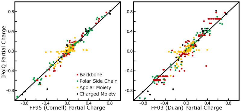
The complete set of 420 partial charges is broken down into backbone atoms, apolar moieties (such as valine side chain, or the methyl groups of lysine side chain), polar moieties, and charged side chain head groups.

Figure 10. Differencesf in the electrostatic potentials due to existing AMBER charge models, and our new model, at points accessible to water molecules.

As in Figure 11, the nuances of the differences may change depending on the exact conformation of any amino acid. IPolQ displays greater polarity than the Cornell (FF95) charge set in the backbone, side chain amides, and tyrosine alcohol groups, and notably less polarity in the serine alcohol group. All of these differences are qualitatively the same, but amplified, when comparing our new charge model to the Duan charge set (FF03).

4.3 Accuracy of the fitted charges for amino acids to the target

While it is an open question whether using the electrostatic field defined in our quantum calculations to derive pairwise interactions between atomic partial charges is an accurate approximation of real molecular electrostatics, the quality with which our fitted charges reproduce the quantum electrostatics is readily answered. Overall, the main-chain, N- and C-terminal amino acids’ partial charges recover the quantum mechanical electrostatic target potentials with a root mean squared error of 1.23, 1.35, and 1.22 kcal/mol-e, respectively, as measured throughout the solvent accessible space within 5Å of the atoms of each amino acid. As expected, the errors were larger for charged amino acids than for neutral and nonpolar ones, but beyond simple observations that stronger electrostatics imply larger errors we looked at the error as a spatial function around individual dipeptide conformations. Some examples of the errors are shown in Figure 11; patterns in the error are apparent at specific chemical groups. The molecular mechanics charges consistently displayed negative error in a cap over the hydroxyl protons of Ser, Thr, and Tyr side chains, and positive error in a cup-shaped region over the oxygen lone pairs, indicating that the true quantum model entails a larger dipole on these alcohol groups than the fitted point charges can afford. Many conformations display lobes of positive error surrounding the backbone carbonyl oxygens, and in some cases the error is concentrated in such a way as to suggest that explicit representation of charge on the carbonyl oxygen’s lone pairs would improve the model. Sulfur atoms, even on the methionine side chain which single-site REsP models consistently fit with low charge, appear to be at the center of some particularly widespread regions of error, in excess of 1.0 kcal/mol-e. Far more common, however, are nebulous but contiguous regions of positive or negative error flanking the molecules on either side. The fact that these regions are typically only 1–2Å thick suggests that, indeed, the long-ranged dipoles of each conformation are being properly represented by the charges, but the electrostatic potential due to these fitted charges is typically in error by 0.25 to 0.5 kcal/mol-e throughout the first solvation shell. Figure 11 shows only regions of space accessible to solvent molecules; as can be seen in other works⁴² the molecular mechanics model predicts the space very close to nuclei and along bonds to be much more electrostatically negative than the true quantum system, reflecting the positive nuclear charges and distributed electron density present in the real system. While this does not generally affect the solute:solvent electrostatic interactions, it may create a bias in 1:4 nonbonded interactions, which fitted dihedral terms must then counteract.

Figure 11. Errors in the fitted electrostatic potential at points accessible to water molecules.

The molecular mechanics charge distributions computed in this study tend to under-polarize hydroxyl and carbonyl groups, and do not capture the multipolar character of sulfur atoms. As evident in the case of phenylalanine dipeptide, even when the fitted charges are all small the molecular mechanics model makes 0.25–0.50 kcal/mol-e errors throughout the first solvation shell. The nuances of the errors may change depending on the exact conformation of any amino acid.

5 Discussion

The IPolQ charge model we present attempts to express the average cost of electronic polarization in the context of static atomic partial charges. The model is general, and because many steps of the protocol are now supported by the mdgx program distributed with AmberTools²⁶ the technique can be applied with some automation. However, the process is iterative at several levels due to the way that changes in nonbonded parameters may require an update to the charge set.

We present a number of simple systems in the Supporting Information to assess the credibility of our approach for treating the average polarization. These examples show that our IPolQ model does make an approximate account of the energetic cost of polarizing a solute as it passes from vacuum to an aqueous environment, and therefore can produce hydration free energies when applied in the context of standard molecular dynamics approaches such as thermodynamic integration. These examples also confirm that our approach only makes a valid representation of the polarization cost in the medium for which it was fitted, in our case pure water. In most simulations the most interesting residues are thoroughly exposed to solvent, or become solvent-exposed as part of the events of interest.⁴³ However, new sets of IPolQ charges with different condensed phase targets may be needed for other applications, such as simulations of ligands in a protein core. It is not clear whether simulations with multiple different charge sets derived by IPolQ for different condensed-phase media would be feasible. However, as biomolecular simulations continue to expand in scope and comprise multiple phases, a more general form of the IPolQ derivation may be in order to address interfaces between condensed-phase environments. Such an approach might also have applications in QM/MM simulations.

In applying Karamertzanis’s arguments²² to derive charges for real molecules, we have also shown that they differ markedly from the recommendations Leontyev et al.,²⁵ even though both approaches seek to implicitly account for the energy of electronic polarization in force fields with fixed charges. Leontyev and colleagues suggest scaling charges in biomolecular simulations by the square root of the electronic screening propensity of the medium, which is roughly 2 for organic media and 1.78 for water (this value is to be distinguished from the macroscopic dielectric constant of water, 78). If our approaches led to similar results, all the charges would be scaled down and the scatter plots in Figure 9 would have slopes of about 0.7, not greater than 1 as they do. The current Amber force fields may have inadvertently conformed to Leontyev’s ideas, however, by scaling the “1:4” electrostatic interactions of atoms connected in the manner (1)A–B–C–D(4) by a factor of 5/6. This factor is a historical artifact and not as large as Leontyev and colleagues prescribe, but it attenuates some of the shortest-ranged, and therefore the strongest, electrostatic interactions in a biomolecular simulation. We will examine the role of the 1:4 scaling factor when making the complete force field for IPolQ.

While the charges presented in Supporting Information are not sufficient to create a new force field, efforts to complete this force field are proceeding. In deriving the charges for all amino acids, we have assumed that updated dihedral parameters, which will be necessary to complete the molecular model, will not adversely affect the hydration free energies of amino acid side chain analogs on which our refitted Lennard-Jones parameters depend. This is a safe assumption, as most of the side chain analogs cannot change shape or charge geometry significantly under any reasonable set of dihedral potentials. Furthermore, because we have a comprehensive set of fitting conformations, a new set of torsional potentials which merely alters the propensity of the system to occupy some of them is unlikely to influence the fitted charges.

Direct comparison of the electrostatics of IPolQ and the earlier Amber charge models of Cornell⁸ and Duan¹⁹ shows that IPolQ portrays proteins with overall more polarity. The only notable exception to this trend is in the hydroxyl groups of serine and threonine side chains; the tyrosine side chain again becomes significantly more polarized under IPolQ. In fact, the Cornell and Duan charge sets model the tyrosine hydroxyl group with significantly less polarity than serine or threonine; in IPolQ, all of these hydroxyls have roughly the same polarity, and the trend is for slightly increasing polarity from serine to threonine to tyrosine. It is also important to note that the hydroxyl oxygen Lennard-Jones radii were reduced in size to accommodate IPolQ. This move made hydration free energies of alcohols fall in line with experiment, and there is then a trend in the negative charges of oxygen on hydroxyl, carbonyl, and carboxylate groups which correlates with a trend in the radii assigned to those atoms. These trends fit with the approach that more negatively charged atoms should be assigned larger van der Waals radii. However, in the case of hydroxyl oxygens the move may also accommodate the fact that all of the alcohols are underpolarized as shown in Figure 11. When the hydroxyl group’s only charge sites are placed on the oxygen and hydrogen nuclei, REsP fitting cannot adequately polarize the hydroxyl group without incurring greater errors elsewhere in the molecular electrostatics.

It is in the context of their failure to reproduce the electrostatic properties of quantum systems that the similarities between molecular mechanics models must be evaluated. The errors with which IPolQ reproduces electrostatics near the molecular surface are often of similar magnitude to the differences between IPolQ and the existing Amber charge sets. It is only outside the first solvation shell that IPolQ, and likely the previous Amber charge models, emulate their quantum mechanical targets with high fidelity and comparisons of the models become valid. A striking example is seen in the case of methionine: IPolQ shows very little difference from either of the Cornell or Duan charge models in modeling the methionine side chain (Figure 10), but all three models are likely making errors such as those shown in Figure 11. In many cases, the differences between the IPolQ and Cornell or other quantum electrostatic targets may have significance for hydration and biomolecular recognition, but the errors inherent to the common nuclear charge framework may overshadow those features.

We hope that IPolQ will extend the lifetime of simple point charge force fields, but it may also be necessary to break the nuclear-centered monopole paradigm. A small basis set of spherically symmetric potentials may be insufficient to represent the electronic structure of molecules, but by adding sites at bond centers or at the locations of other hybrid orbitals, a molecular mechanics model can much better reflect the electron density seen in quantum calculations. The analysis presented in Figure 11 can determine the locations of such extra sites, and more accurate charge models will, in turn, improve our ability to evaluate which quantum mechanical targets are the best for creating a specific class of force field.

Table 1. Hydration free energies for ionic amino acid side chains.

All values are reported in kcal/mol and do not include any estimate of the air/water interface potential, as appropriate for comparison to simulations with infinite electrostatics and periodic boundary conditions. Values listed in bold are target hydration free energies to be obtained through molecular mechanics simulations.

Energy	Asp	Glu	Hip	Lys	Arg
1	341.5b	340.4c	220.1d	211.9d	235.2a,d
3+5	−6.7e	−6.5e	−52.8	−59.5	46.5
7	−252.5f
8	6.5h	6.6h	10.2g	14.5g	18.3g
4+6	−89.2	−87.8	−10.2e	−4.4e	−10.9e

^aThis value is estimated as the known experimental basicity for guanidine plus the difference in G2 estimates for the basicity of N-propylguanidine and guanidine.

^bCumming and Kebarle, 1978³⁰

^cCaldwell et al., 1989⁴⁴

^dHunter and Lias, 1998⁴⁵

^eWolfenden et al., 1981³³

^fGrossfield et al., 2003³⁴

^gKyte, 1995⁴⁶

^hCRC Handbook of Chemistry and Physics, 91st Ed.⁴⁷

Table 2. Changes in Lennard-Jones parameters made to bring computed HFEs in line with experiment.

These changes, as described in the main text, were implemented to bring the HFEs of amino acid side chain analogs, as computed by thermodynamic integration, into agreement with experimental data or values inferred from experiment. Only σ, not ε, parameters were altered.

Atom Type	Instances	Original σ, Å	New σ, Å
OH	Hydroxyl oxygens	3.0664	2.9578
O	Amide oxygens	2.9600	3.2072
N9	Primary amide nitrogens	3.2500	3.4924
SH	Thiol sulfur	3.5636	3.3498
O2	Carboxylate oxygen	2.9600	3.3150
N3	Terminal and Lys amino nitrogen	3.2500	3.0061

References

- 1.Ponder J, Wu C, Ren P, Pande V, JDC, MJS, Haque I, Mobley D, Lambrecht D, DiStasio J, RA, Head-Gordon M, Clark G, Johnson M, Head-Gordon T. J Phys Chem B. 2010;114:2549–2564. doi: 10.1021/jp910674d. [DOI] [PMC free article] [PubMed] [Google Scholar]
- 2.Cisneros G, Tholander NI, Parisel O, Darden T, Elking D, Perera L, Piquemal JP. Int J Quantum Chem. 2008;108:1905–1912. doi: 10.1002/qua.21675. [DOI] [PMC free article] [PubMed] [Google Scholar]
- 3.Xie W, Orozco M, Truhlar D, Gao J. J Chem Theory Comput. 2009;5:459–467. doi: 10.1021/ct800239q. [DOI] [PMC free article] [PubMed] [Google Scholar]
- 4.Jorgensen W, Chandrasekhar D, Madura J, Impey R, Klein M. J Chem Phys. 1983;79:926–935. [Google Scholar]
- 5.Berendsen H, Grigera J, Straatsma T. J Phys Chem. 1987;91:6269–6271. [Google Scholar]
- 6.Price D, Brooks C., III J Chem Phys. 2004;121:10096–10103. doi: 10.1063/1.1808117. [DOI] [PubMed] [Google Scholar]
- 7.MacKerell A, Jr, et al. J Phys Chem B. 1998;102:3586–3616. doi: 10.1021/jp973084f. [DOI] [PubMed] [Google Scholar]
- 8.Cornell W, Cieplak P, Bayly C, Gould I, Merz KJ, Ferguson D, Spellmeyer D, Fox T, Caldwell J, Kollman P. J Am Chem Soc. 1995;117:5179–5197. [Google Scholar]
- 9.UE, Perera L, Berkowitz M, Darden T, Lee H, Pedersen L. J Chem Phys. 1995;103:8577–8593. [Google Scholar]
- 10.Phillips J, Braun R, Wang W, Gumbart J, Tajkhorshid E, Villa E, Chipot C, Skeel R, Kalé L, Schulten K. J Comp Chem. 2005;26:1781–1802. doi: 10.1002/jcc.20289. [DOI] [PMC free article] [PubMed] [Google Scholar]
- 11.Hess B, Kutzner C, van der Spoel D, Lindahl E. J Chem Theory Comput. 2008;4:435–447. doi: 10.1021/ct700301q. [DOI] [PubMed] [Google Scholar]
- 12.Shan Y, Kim E, Eastwood M, Dror R, Seeliger M, Shaw D. J Am Chem Soc. 2011;133:9181–9183. doi: 10.1021/ja202726y. [DOI] [PMC free article] [PubMed] [Google Scholar]
- 13.Zwier M, Chong L. Curr Opin Pharmacol. 2010;10:745–752. doi: 10.1016/j.coph.2010.09.008. [DOI] [PubMed] [Google Scholar]
- 14.Lindorff-Larsen K, Maragakis P, Piana S, Eastwood M, Dror R, Shaw D. PLoS ONE. 2012;7:e32131. doi: 10.1371/journal.pone.0032131. [DOI] [PMC free article] [PubMed] [Google Scholar]
- 15.Freddolino P, Park S, Roux B, Schulten K. Biophys J. 2009;96:3772–3780. doi: 10.1016/j.bpj.2009.02.033. [DOI] [PMC free article] [PubMed] [Google Scholar]
- 16.Cerutti D, Freddolino P, Duke R, Case D. J Phys Chem B. 2010;114:12811–12824. doi: 10.1021/jp105813j. [DOI] [PMC free article] [PubMed] [Google Scholar]
- 17.Bayly C, Cieplak P, Cornell W, Kollman P. J Phys Chem. 1993;97:10269–10280. [Google Scholar]
- 18.Kimura S, Rajamani R, Langley D. J Chem Phys. 2011;135:231101. doi: 10.1063/1.3671638. [DOI] [PubMed] [Google Scholar]
- 19.Duan Y, Wu C, Chowdhury S, Lee M, Xiong G, Zhang W, Yang R, Cieplak P, Luo R, Lee T. J Comput Chem. 2003;24:1999–2012. doi: 10.1002/jcc.10349. [DOI] [PubMed] [Google Scholar]
- 20.Horn H, Swope W, Pitera J, Madura J, Dick T, Hura G, Head-Gordon T. J Chem Phys. 2004;120:9665–9678. doi: 10.1063/1.1683075. [DOI] [PubMed] [Google Scholar]
- 21.Shaw K, Woods C, Mulholland A. J Phys Chem Lett. 2010;1:219–223. [Google Scholar]
- 22.Karamertzanis P, Raiteri P, Galindo A. J Chem Theory Comput. 2010;6:3153–3161. doi: 10.1021/ct900693q. [DOI] [PubMed] [Google Scholar]
- 23.Swope W, Horn H, Rice J. J Phys Chem B. 2010;114:8621–8630. doi: 10.1021/jp911699p. [DOI] [PubMed] [Google Scholar]
- 24.Swope W, Horn H, Rice J. J Phys Chem B. 2010;114:8631–8645. doi: 10.1021/jp911701h. [DOI] [PubMed] [Google Scholar]
- 25.Leontyev V, Stuchebrukhov A. Phys Chem Chem Phys. 2011;13:2613–2626. doi: 10.1039/c0cp01971b. [DOI] [PubMed] [Google Scholar]
- 26.Case D, Cheatham T, Darden T, Gohlke H, Luo R, Merz KJ, Onufriev A, Simmer-ling C, Wang B, Woods R. J Comput Chem. 2005;26:1668–1688. doi: 10.1002/jcc.20290. [DOI] [PMC free article] [PubMed] [Google Scholar]
- 27.Steinbrecher T, Mobley D, Case D. J Chem Phys. 2007;127:214108. doi: 10.1063/1.2799191. [DOI] [PubMed] [Google Scholar]
- 28.Pearson R. J Am Chem Soc. 1986;108:6109–6114. [Google Scholar]
- 29.Steinbrecher T, Latzer J, Case D. J Chem Theory Comput. 2012;8:4405–4412. doi: 10.1021/ct300613v. [DOI] [PMC free article] [PubMed] [Google Scholar]
- 30.Cumming J, Kebarle P. Can J Chem. 1978;56:1–9. [Google Scholar]
- 31.Taft R, Topsom R. Prog Phys Org Chem. 1987;103:1. [Google Scholar]
- 32.Fujio M, McIver RJ, Taft R. J Am Chem Soc. 1981;103:4017–4029. [Google Scholar]
- 33.Wolfenden R, Anderson L, Cullis P, Southgate C. Biochemistry. 1981;20:849–855. doi: 10.1021/bi00507a030. [DOI] [PubMed] [Google Scholar]
- 34.Grossfield A, Ren P, Ponder J. J Am Chem Soc. 2003;125:15671–15682. doi: 10.1021/ja037005r. [DOI] [PubMed] [Google Scholar]
- 35.Dunning TJ, Peterson K, Wilson A. J Chem Phys. 2001;114:9244–9253. [Google Scholar]
- 36.Woon D, Dunning TJ. J Chem Phys. 1993;98:1358–1371. [Google Scholar]
- 37.Kendall R, Dunning TJ, Harrison R. J Chem Phys. 1992;96:6796–6806. [Google Scholar]
- 38.Dunning TJ. J Chem Phys. 1989;90:1007–1023. [Google Scholar]
- 39.Hornak V, Abel R, Okur A, Strockbine B, Roitberg A, Simmerling C. Proteins. 2006;65:712–725. doi: 10.1002/prot.21123. [DOI] [PMC free article] [PubMed] [Google Scholar]
- 40.Badyal Y, Saboungi M, Price D, Shastri S, Haeffner D, Soper A. J Chem Phys. 2000;112:9206–9208. [Google Scholar]
- 41.Wang J, Cieplak P, Kollman P. J Comp Chem. 2000;21:1049–1074. [Google Scholar]
- 42.Mobley D, Liu S, Cerutti D, Swope W, Rice J. J Comput Aided Mol Des. 2012;26:551–562. doi: 10.1007/s10822-011-9528-8. [DOI] [PMC free article] [PubMed] [Google Scholar]
- 43.Schames J, Henchamn R, Siegel J, Sotriffer C, Ni H, McCammon J. J Med Chem. 2004;47:1879–1881. doi: 10.1021/jm0341913. [DOI] [PubMed] [Google Scholar]
- 44.Caldwell G, Renneboog R, Kebarle P. Can J Chem. 1989;67:611–618. [Google Scholar]
- 45.Hunter E, Lias S. J Phys Chem Ref Data. 1998;27:413–656. [Google Scholar]
- 46.Kyte J. Structure in Protein Chemistry. Garland Publishing, Inc; New York: 1995. [Google Scholar]
- 47.Haynes W, editor. CRC Handbook of Chemistry and Physics. 91. CRC Press; Boston: 2010. [Google Scholar]
- 48.Wolfenden R. Biochemistry. 1978;17:201–204. doi: 10.1021/bi00594a030. [DOI] [PubMed] [Google Scholar]
Associated Data
This section collects any data citations, data availability statements, or supplementary materials included in this article.