The Relevance Voxel Machine (RVoxM): A Self-tuning Bayesian Model for Informative Image-based Prediction

Abstract

This paper presents the Relevance Voxel Machine (RVoxM), a dedicated Bayesian model for making predictions based on medical imaging data. In contrast to the generic machine learning algorithms that have often been used for this purpose, the method is designed to utilize a small number of spatially clustered sets of voxels that are particularly suited for clinical interpretation. RVoxM automatically tunes all its free parameters during the training phase, and offers the additional advantage of producing probabilistic prediction outcomes. We demonstrate RVoxM as a regression model by predicting age from volumetric gray matter segmentations, and as a classification model by distinguishing patients with Alzheimer’s disease from healthy controls using surface-based cortical thickness data. Our results indicate that RVoxM yields biologically meaningful models, while providing state-of-the-art predictive accuracy.

I. Introduction

Medical image-based prediction aims at estimating a clinically or experimentally relevant quantity directly from individual medical scans. In a typical scenario, the properties of prediction models are learned from so-called training data – a set of images for which the quantity of interest is known. The trained models can then be applied to make predictions on new cases. In so-called image-based regression problems, the quantity to be estimated is continuously valued, such as a score evaluating a subject’s brain maturity. In other cases, the aim is to predict a discrete value indicating one of several conditions, such as a clinical diagnosis, which is a classification problem.

Image-based prediction models derive their predictive power from considering all image voxels simultaneously, distilling high prediction accuracy from many voxel-level measurements that are each only weakly predictive when considered individually. This approach is fundamentally different from more traditional ways of relating image content to the biomedical context, such as voxel- and deformation-based morphometry [1]–[3], cortical thickness analysis [4], or voxel-level fMRI analysis [5], in which maps of affected anatomical areas are generated by merely considering each location separately. Unlike such “mapping” approaches, prediction methods explore patterns of association between voxels, offering powerful new analysis tools in such applications as “mind reading” [6], [7], studying neural information processing [8]–[10], image-based clinical diagnosis [11]–[16], and examining global patterns associated with healthy development, aging, pathology or other factors of interest [17], [18].

The principal difficulty in obtaining good regression and classification models for medical imaging data is the enormous number of voxels in images, which leads to two interconnected modeling challenges. First, since the number of training images is typically several orders of magnitude smaller than the number of voxels, the complexity of voxel-based prediction models needs to be strictly controlled in order to avoid so-called “over-fitting” to the training data, where small modeling errors in the training images are obtained at the expense of poor prediction performance on new cases. Second, the aim is often not only to predict well, but also to obtain insight into the anatomical or functional variations that are driving the predictions – in some applications, such as task-related fMRI, this is even the primary result. Interpreting complex patterns of association between thousands of image voxels is a highly challenging task, especially when the results indicate that all the voxels are of importance simultaneously; when the voxels contributing most to the predictions appear randomly scattered throughout the image area; or when the relevant inter-location relationships are non-linear in nature [19]–[22].

Various approaches for restricting model complexity in medical image-based prediction have been proposed in the literature, often with the adverse effect of reducing biological interpretability. Some methods only allow a selected few voxels to contribute to the prediction, either by performing voxel-wise tests a priori [7] or by pruning less predictive voxels as part of a larger modeling process [23]–[25]. Others aim at using spatially connected patches of voxels as “features” instead of individual voxels themselves, either by averaging over a priori defined anatomical structures [7], [20], [26], [27], or by trying to cluster neighboring voxels in such a way that good prediction performance is obtained [22]. Yet others rely directly on more off-the-shelf techniques, for instance using only a few of all the available training subjects in sparse kernel-based machine learning methods [14], or reducing feature dimensionality by spatial smoothing, image downsampling, or principal component analysis [9], [28], [29].

In order to obtain prediction models that are expressly more biologically informative, some authors have started to exploit the specific spatial, functional, or temporal structure of their imaging data as a basis for regularization [30]–[37]. Building on this idea, we propose in this paper the Relevance Voxel Machine (RVoxM), a novel Bayesian method for image-based prediction that combines excellent prediction accuracy with intuitive interpretability of its results. RVoxM considers a family of probabilistic models to express that (1) not all image locations may be equally relevant for making predictions about a specific experimental or clinical condition, and (2) image areas that are somehow biologically connected may be more similar in their relevance for prediction than completely unrelated ones. It then assesses which model within this family explains the training data best, using the fact that simple models that sufficiently explain the data without unnecessary complexity are automatically preferred in Bayesian analysis [38]. As we shall see, this technique yields models that are sparse – only a small subset of voxels is actually used to compute predictions – as well as spatially smooth –in our experiments we used spatial proximity as a measure of biological connectivity. Such models are easier to interpret than speckles of isolated voxels scattered throughout the image area, and at the same time have an adequately reduced number of degrees of freedom to avoid over-fitting to the training data.

Compared to many existing image-based prediction methods, our Bayesian approach has several advantages:

• Simultaneous regularization, feature selection, and biological consistency: Rather than computing discriminative features in a separate pre-processing step [22], [25], [28], or using post-processing to analyze which subset of voxels contributes most to the predictions [9], [34], [37], the proposed method automatically determines which voxels are relevant – and uses only these voxels to make predictions – in a single consistent modeling framework. In line with anatomical expectations, the obtained maps of “relevance voxels” have spatial structure, facilitating biological interpretation and contributing to the regularization of the method.

• Self-tuning: The proposed method automatically tunes all the parameters of the prediction model, allowing the model to adapt to whatever degree of spatial sparseness and smoothness is indicated by the training data. In contrast, other image-based prediction methods rely on regularization parameters that need to be determined externally, either by manual selection [30], [33], [34] or using cross-validation [22], [26], [28], [31], [35], [37]. As illustrated in [39], the latter can be extremely challenging when several regularization parameters need to be determined simultaneously.

• Probabilistic predictions: In contrast to the decision machines [40] widely used in biomedical image classification, which aim to minimize the risk of misclassification, the method we propose computes posterior probabilities of class membership, from which optimal class assignments can subsequently be derived. The ability to obtain probabilistic predictions rather than “hard” decisions is important for building real-world diagnostic systems, in which image-based evidence may need to be combined with other sources of information to obtain a reliable diagnosis, and the risk of making false positive diagnoses needs to be weighed differently than that of false negative ones [41].

We originally presented RVoxM in a short conference paper that only dealt with the regression problem [42]. The current manuscript extends the theory to encapsulate classification, contains more details on theoretical derivations, and includes more extensive experimental results.

A reference Matlab implementation of the method is freely available from the authors.

II. RVoxM for Regression

For regression problems, the aim is to predict a real-valued target variable t ∈ ℝ from an image x = (x₁, …, x_M−1, 1)^T, where x_i ∈ ℝ denotes a voxel-level measurement at the voxel indexed by i, and M − 1 is the total number of voxels. For notational convenience in the remainder, an extra element with value 1 is also included to account for constant offsets in our predictions.

We use a standard linear regression model for t, defined by the Gaussian conditional distribution

$$p(t\mid \mathbf{x},\mathbf{w},\beta )=\mathcal{N}(t\mid y(\mathbf{x};\mathbf{w}),{\beta }^{-1})$$ (1)

with variance β⁻¹ and mean

$$y(\mathbf{x};\mathbf{w})=\sum _{i=1}^{M-1}{x}_i{w}_i+w_M={\mathbf{w}}^{\text{T}}\mathbf{x},$$ (2)

where w = (w₁ · · · w_M )^T ∈ ℝ^M denotes a vector of unknown, adjustable “weights” encoding the strength of each voxel’s contribution to the prediction of t. In order to complete the model, we also define a prior on these weights that expresses our prior anatomical expectations that not all locations in the image may be equally predictive, and that biologically related areas may be more similarly predictive than completely unrelated ones. In particular, we use a prior of the form

$$p(\mathbf{w}\mid \mathit{\alpha },\lambda )\propto exp\left(-\frac{1}{2}\sum _{i=1}^M{\alpha }_i{w}_i^2-\frac{\lambda }{2}{\left|\right|\mathbf{\Gamma }\mathbf{w}\left|\right|}^2\right),$$ (3)

where α = (α₁, …, α_M )^T and λ are so-called hyper-parameters, and Γ is a matrix chosen so that elements of the vector Γw evaluate to large values when biologically connected voxels happen to have very different weights in w, effectively making such configurations a priori less likely.

The role of the hyper-parameters in eq. (3) is to express a wide range of regression models that can each be tried and tested, ranging from very complex models with many degrees of freedom (when all the hyper-parameters are set to small values) to heavily regularized ones with limited expressive power (when all the hyper-parameters are large). It is these hyper-parameters that are automatically learned from training data, as will be explained in section II-A, allowing the data to select the appropriate form of the model. When a large value for λ is selected, the model encodes a preference for configurations of w in which biologically connected voxels have similar weights. At the same time, setting some of the hyper-parameters α_i to very large values (infinity in theory) will clamp the values for the weights w_i in the corresponding voxels to zero, effectively “switching off” the contribution of these voxels to the prediction and removing them from the model. This ability for the data to determine which inputs should influence the predictions is similar to the Automatic Relevance Determination (ARD) mechanism [43] used in the Relevance Vector Machine (RVM) [44]; in fact, for λ = 0 our model reduces to an RVM with the voxel-wise intensities stacked as basis functions.

For the remainder of this paper, we will use a matrix Γ that simply encourages local spatial smoothness of w as a proxy for biological connectivity. In particular, we will use a sparse matrix with as many rows as there are pairs of neighboring voxels in the image; for a pair {i, j}, the corresponding row has zero entries everywhere expect for the i^thand j^th column, which have entries −1 and 1, respectively. To simplify notation in subsequent sections, we re-write eq. (3) in the form

$$p(\mathbf{w}\mid \mathit{\alpha },\lambda )=\frac{{\mid \mathbf{P}\mid }^{1/2}}{{(2\pi )}^{M/2}}exp(-\frac{1}{2}{\mathbf{w}}^{\text{T}}\mathbf{Pw}),$$ (4)

which shows that the prior is a zero-mean Gaussian with inverse covariance P = diag(α) + λL, where L = Γ^TΓ is also known as the Laplacian matrix in graph theory.

While our choice of Γ here simply penalizes spatial gradients in w, it is worth noting that more advanced measures of biological connectivity can easily be integrated into the model as well – each with its own hyper-parameter that is automatically determined. Examples of such measures might include left-right symmetry relationships, as well as voxel-to-voxel connectivity strengths derived from functional image studies or based on detailed anatomical segmentations.

A. Training

Given a set of N training images x_n, n = 1, …, N with corresponding target values t_n, n = 1, …, N, we can determine the appropriate form of the regression function by estimating the hyper-parameters that maximize the so-called marginal likelood function, which expresses how probable the observed training data is for different settings of the hyper-parameters. Figure 1 shows the graphical model which depicts the dependency relationship between the variables. Collecting all the training images in the N × M “design” matrix X = [x₁, · · ·, x_N ]^T, and the corresponding target values in the vector t = (t₁, …, t_N )^T, the marginal likelihood function is obtained by integrating out the weight parameters, yielding [41]

Fig. 1.

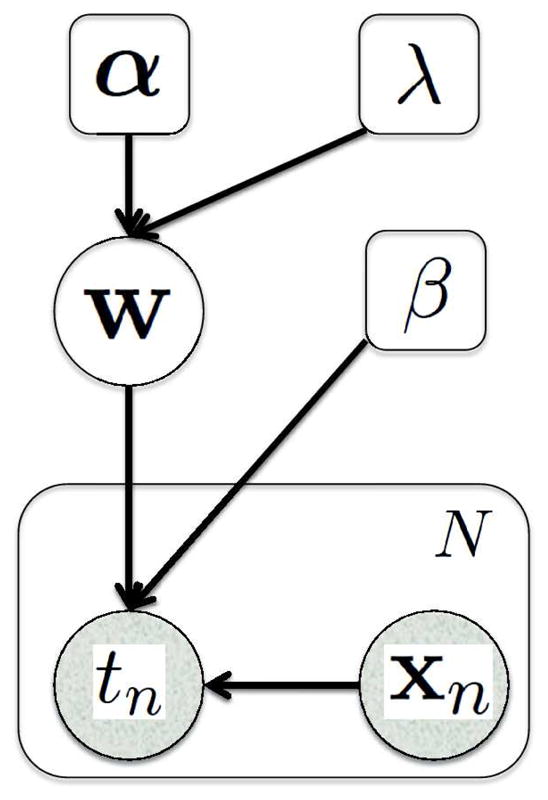
Graphical representation of the regression model with N training subjects. Random variables are in circles and parameters are in squares. Shaded variables are observed. The plate indicates replication of N times.

$$\begin{array}{l}p(\mathbf{t}\mid \mathbf{X},\mathit{\alpha },\lambda ,\beta )={\int }_{\mathbf{w}}\left(\prod _{n=1}^{N}p(t_n\mid {\mathbf{x}}_n,\mathbf{w},\beta )\right)p(\mathbf{w}\mid \mathit{\alpha },\lambda )\text{d}\mathbf{w}\\ =\mathcal{N}(\mathbf{t}\mid \mathbf{0},\mathbf{C}),\end{array}$$ (5)

where

$$\mathbf{C}={\beta }^{-1}\mathbf{I}+{\mathbf{XP}}^{-1}{\mathbf{X}}^{\text{T}}.$$ (6)

Our goal is now to maximize eq. (5) with respect to the hyper-parameters α, λ, and β – known in the literature as the evidence procedure [45], type-II maximum likelihood estimation [46], or restricted maximum likelihood estimation [47].

We follow a heuristic optimization strategy similar to the one proposed in [45], which has also been used to train RVM regression models [44]. In particular, we maximize ln p(t|X, α, λ, β) – which is equivalent to maximizing p(t|X, α, λ, β) but computationally more convenient – by observing that its derivatives to the hyper-parameters are given by the following expressions (see Appendix A for detailed derivations):

$$\frac{\partial lnp(\mathbf{t}\mid \mathbf{X},\mathit{\alpha },\lambda ,\beta )}{\partial {\alpha }_i}=\frac{1}{2{\alpha }_i}(1-{\alpha }_i{\mathrm{\sum }}_{ii}-\lambda {({\mathbf{P}}^{-1}\mathbf{L})}_{ii}-{\alpha }_i{\mu }_i^2)$$ (7)

$$\frac{\partial lnp(\mathbf{t}\mid \mathbf{X},\mathit{\alpha },\lambda ,\beta )}{\partial \beta }=\frac{1}{2}\left(\frac{N}{\beta }-\text{trace}(\mathbf{X}\mathbf{\sum }{\mathbf{X}}^{\text{T}})-{\left|\right|\mathbf{t}-\mathbf{X}\mathit{\mu }\left|\right|}^2\right)$$ (8)

$$\frac{\partial lnp(\mathbf{t}\mid \mathbf{X},\mathit{\alpha },\lambda ,\beta )}{\partial \lambda }=-\frac{1}{2}\left(\text{trace}\left((\mathbf{\sum }-{\mathbf{P}}^{-1})\mathbf{L}\right)+{\mathit{\mu }}^{\text{T}}\mathbf{L}\mathit{\mu }\right),$$ (9)

where Σ_ii is the i^th diagonal component of the matrix

$$\mathbf{\sum }={(\beta {\mathbf{X}}^{\text{T}}\mathbf{X}+\mathbf{P})}^{-1}$$ (10)

and μ_i the i^th component of the vector

$$\mathit{\mu }=\beta \mathbf{\sum }{\mathbf{X}}^{\text{T}}\mathbf{t}.$$ (11)

Because their derivatives are zero at a maximum of the objective function, one strategy of optimizing for α and β is to equate eq. (7) and (8) to zero and re-arranging, yielding the following re-estimation equations:

$${\alpha }_i^{\text{new}}=\frac{1-{\alpha }_i{\mathbf{\sum }}_{ii}-\lambda {({\mathbf{P}}^{-1}\mathbf{L})}_{ii}}{{\mu }_i^2}$$ (12)

and

$${\beta }^{\text{new}}=\frac{N-\text{trace}(\beta \mathbf{X}\mathbf{\sum }{\mathbf{X}}^{\text{T}})}{{\left|\right|\mathbf{t}-\mathbf{X}\mathit{\mu }\left|\right|}^2}.$$ (13)

In Appendix B, we show that both eq. (12) and (13) are guaranteed to yield non-negative ${\alpha }_i^{\text{new}}$ and β^new.

For the hyper-parameter λ, we use a standard gradient-ascent approach, yielding the following update equation:

$${\lambda }^{\text{new}}=\lambda -\kappa \left(\text{trace}\left((\mathbf{\sum }-{\mathbf{P}}^{-1})\mathbf{L}\right)+{\mathit{\mu }}^{\text{T}}\mathbf{L}\mathit{\mu }\right)$$ (14)

where κ is an appropriate step-size.

Training now proceeds by choosing initial values for the hyper-parameters α, β, and λ, and then iteratively recomputing Σ and μ (eq. (10) and (11)) and the hyper-parameters (eq. (12), (13), and (14)), each in turn, until convergence. In our implementation, we initialize with α_i = 1, ∀i, λ = 1, and β = 10/variance(t). We monitor the value of the objective function ln p(t|X, α, β, λ) at each iteration, and terminate when the change over the previous iteration is below a certain tolerance. Section IV provides detailed pseudo-code for this algorithm, optimized for the computational and memory requirements of image-sized problems.

Although we have no theoretical guarantees that the proposed update equations for the hyper-parameters improve the objective function at each iteration, our experiments indicate that this is indeed the case.

B. Prediction

Once we have learned suitable hyper-parameters α^*, λ^*, and β^* from the training data, we can make predictions about the target variable t for a new input image x by evaluating the predictive distribution

$$p(t\mid \mathbf{x},\mathbf{X},\mathbf{t},{\mathit{\alpha }}^{\ast },{\lambda }^{\ast },{\beta }^{\ast })={\int }_{\mathbf{w}}p(t\mid \mathbf{x},\mathbf{w},{\beta }^{\ast })p(\mathbf{w}\mid \mathbf{X},\mathbf{t},{\mathit{\alpha }}^{\ast },{\lambda }^{\ast })\text{d}\mathbf{w},$$ (15)

where p(t|x, w, β^*) is given by eq. (1) and

$$\begin{array}{l}p(\mathbf{w}\mid \mathbf{X},\mathbf{t},{\mathit{\alpha }}^{\ast },{\lambda }^{\ast })=\frac{\left({\prod }_{n=1}^{N}p(t_n\mid {\mathbf{x}}_n,\mathbf{w},{\beta }^{\ast })\right)p(\mathbf{w}\mid {\mathit{\alpha }}^{\ast },{\lambda }^{\ast })}{p(\mathbf{t}\mid \mathbf{X},{\mathit{\alpha }}^{\ast },{\lambda }^{\ast },{\beta }^{\ast })}\\ =\mathcal{N}(\mathbf{w}\mid {\mathit{\mu }}^{\ast },{\mathbf{\sum }}^{\ast })\end{array}$$ (16)

is the posterior distribution over the voxel weights. Σ^* and μ^* are defined by eq. (10) and (11), in which α, λ, and β have been set to their optimized values.

It can be shown that the predictive distribution of eq. (15) is a Gaussian with mean

$${\mathit{\mu }}^{\ast \text{T}}\mathbf{x}$$ (17)

and variance 1/β^*+x^TΣ^*x [41]. In practice, we will therefore use eq. (17) for making predictions, i.e., the linear regression model of eq. (2) where the voxel weights w have been set to μ^*. As we shall see in section V, most of these weights will typically be zero with the remaining voxels appearing in spatially clustered patches, immediately highlighting which image areas are driving the predictions.

III. RVoxM for Classification

In image-based binary classification, the aim is to predict a binary variable b ∈ {0, 1} from an individual image x. As in regression, we define the linear model

$$y(\mathbf{x};\mathbf{w})={\mathbf{w}}^{\text{T}}\mathbf{x},$$ (18)

but transform the output by a logistic sigmoid function

$$\sigma (y)=\frac{1}{1+exp(-y)}$$ (19)

to map it into the interval [0, 1]. We can then use σ(y(x; w)) to represent the probability that b = 1 (Bernoulli distribution):

$$p(b\mid \mathbf{x},\mathbf{w})=\sigma {(y(\mathbf{x};\mathbf{w}))}^b{(1-\sigma (y(\mathbf{x};\mathbf{w})))}^{1-b},$$ (20)

and complete the model by using the same prior on w as in the regression case (eq. (3)). Note that, unlike in the regression model, there is no hyper-parameter β for the noise variance here.

Training the classification model entails estimating the hyper-parameters that maximize the marginal likelihood function

$$p(\mathbf{b}\mid \mathbf{X},\mathit{\alpha },\lambda )={\int }_{\mathbf{w}}p(\mathbf{b}\mid \mathbf{X},\mathbf{w})p(\mathbf{w}\mid \mathit{\alpha },\lambda )\text{d}\mathbf{w},$$ (21)

where

$$p(\mathbf{b}\mid \mathbf{X},\mathbf{w})=\prod _{n=1}^{N}p(b_n\mid {\mathbf{x}}_n,\mathbf{w})$$

and b = (b₁, …, b_N )^T contains the known, binary outcomes for all the training images x_n, n = 1, …, N. In contrast to the regression case, the integration over w cannot be evaluated analytically, and we need to resort to approximations. In Appendix C, we show that around a current hyper-parameter estimate {α̃, λ̃}, we can map the classification problem to a regression one:

$$lnp(\mathbf{b}\mid \mathit{\alpha },\lambda )\simeq ln\mathcal{N}(\stackrel{\sim }{\mathbf{t}}\mid \mathbf{0},\stackrel{\sim }{\mathbf{C}})+\text{const},$$ (22)

where we have defined a covariance matrix

$$\stackrel{\sim }{\mathbf{C}}={\stackrel{\sim }{\mathbf{B}}}^{-1}+{\mathbf{XP}}^{-1}{\mathbf{X}}^{\text{T}}$$

and local regression “target variables”

$$\stackrel{\sim }{\mathbf{t}}=\mathbf{X}{\stackrel{\sim }{\mathbf{w}}}_{\text{MP}}+{\stackrel{\sim }{\mathbf{B}}}^{-1}(\mathbf{b}-\stackrel{\sim }{\mathbf{\sigma }})$$

with the inverse variances of subject-specific regression “noise” β̃_n = σ̃_n(1 − σ̃_n) collected in the diagonal matrix B̃ = diag(β̃₁, …, β̃_N ), and ${\stackrel{\sim }{\sigma }}_n=\sigma ({\mathbf{x}}_n^{\text{T}}{\stackrel{\sim }{\mathbf{w}}}_{\text{MP}})$ and σ̃ = (σ̃₁ …, σ̃_N )^T. In these equations, w̃_MP are the “most probable” voxel weights given the hyper-parameters {α̃, λ̃}:

$${\stackrel{\sim }{\mathbf{w}}}_{\text{MP}}=arg\underset{\mathbf{w}}{max}p(\mathbf{w}\mid \mathbf{X},\mathbf{b},\stackrel{\sim }{\mathit{\alpha }},\stackrel{\sim }{\lambda }),$$ (23)

which involves solving a concave optimization problem. As detailed in Appendix C, we use Newton’s method to perform this optimization.

Using the local mapping of eq. (22), learning the hyper-parameters now proceeds by iteratively using the regression update equations (12) and (14), but with μ and Σ defined as

$$\mathit{\mu }=\mathbf{\sum }{\mathbf{X}}^{\text{T}}\stackrel{\sim }{\mathbf{B}}\stackrel{\sim }{\mathbf{t}}.$$ (24)

and

$$\mathbf{\sum }={({\mathbf{X}}^{\text{T}}\stackrel{\sim }{\mathbf{B}}\mathbf{X}+\mathbf{P})}^{-1}.$$ (25)

Once we have learned the hyper-parameters α^* and λ^* this way, we can make predictions about the target variable b for a new input image x by evaluating the predictive distribution

$$\begin{array}{l}p(b=1\mid \mathbf{x},\mathbf{X},\mathbf{t},{\mathit{\alpha }}^{\ast },{\lambda }^{\ast })={\int }_{\mathbf{w}}p(b=1\mid \mathbf{x},\mathbf{w})p(\mathbf{w}\mid \mathbf{X},\mathbf{t},{\mathit{\alpha }}^{\ast },{\lambda }^{\ast })\text{d}\mathbf{w}\\ \simeq \sigma (\tau {\mathit{\mu }}^{\ast \text{T}}\mathbf{x}),\end{array}$$ (26)

where τ = (1 + πx^TΣ^*x/8)^−1/2, and μ^* and Σ^* are defined by eq. (24) and (25) in which the hyper-parameters have been set to their optimized values. The approximation in eq. (26) is based on the so-called Laplace approximation and on the similarity between the logistic sigmoid function and the probit function; see [41], pp. 217–220, for details. Eq. (26) can be thresholded at 0.5 to obtain a discrete prediction.

IV. Implementation

In most applications where RVoxM will be useful, the number of voxels to consider (M) is so large (e.g., 10⁴ or 10⁵) that a naive implementation of the proposed training update equations is computationally prohibitive – computing Σ alone already involves inverting a dense M × M matrix, which can take (M³) time.

One approach to alleviate the computational burden is to exploit the sparsity of the matrix P and use Woodbury’s matrix identity [48] to compute Σ as

$$\mathbf{\sum }={\mathbf{P}}^{-1}-{\mathbf{Z}}^{\text{T}}{\mathbf{C}}^{-1}\mathbf{Z},$$ (27)

where Z = XP⁻¹. Since P is sparse (with a the number of nonzero entries in each row being independent of M), the complexity of computing P⁻¹ and subsequently Z is (M²) and (MN), respectively. A naive computation of C using eq. (6) is (M²N). Yet re-writing C as

$$\mathbf{C}={\beta }^{-1}\mathbf{I}+{\mathbf{ZX}}^{\text{T}},$$ (28)

reduces the complexity of computing C to (N²M). Inverting C is (N³). Putting all this together, we can compute Σ using eq. (27) in (M² + MN + N²M + N³) time. Since the number of available training subjects (N) is typically in the hundreds at best, in practice this means a reduction in computation time from (M³) to (M²).

Since M is so large, even an (M²) complexity is still a heavy computational burden. In practice, however, many of the α_i’s tend to grow very large, effectively switching off the contribution of the corresponding voxels. We therefore resort to the type of greedy algorithm originally used for RVM training [44], whereby once a voxel has been switched off (i.e., its α_i has become larger than some threshold –in our implementation 10¹² – it gets permanently discarded from the remaining computations. This provides a significant acceleration of the learning algorithm, as gradually more and more voxels are pruned from the model. To see how voxels can be removed from the computations, consider that P_ii → ∞ if α_i → ∞, and, as a result, the i’th row and i’th column of P⁻¹ and Σ become zero vectors and μ_i → 0. Consequently, the update equations for the hyper-parameters are unaffected by simply deleting the i’th column from X, and both the i’th column and the i’th row from Σ and P⁻¹.

Finally, rather than manipulating the dense M × M matrices Σ and P⁻¹ in their entirety, it is possible to compute their relevant contributions only one row at a time, avoiding the need to explicitly store such prohibitively large matrices.

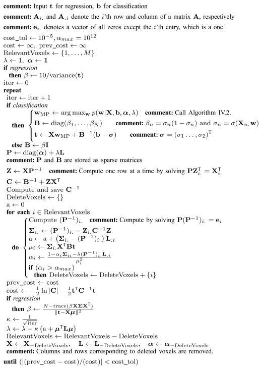
Algorithm IV.1 provides pseudo-code for a RVoxM training procedure that has been optimized along the lines described above. For the classification case, a subroutine that optimizes for w_MP is given in Algorithm IV.2.

Algorithm IV.1.

RVoxM_Training (L, X, t or b)

Algorithm IV.2.

Optimize_w(X, b, w, P, RelevantVoxels)

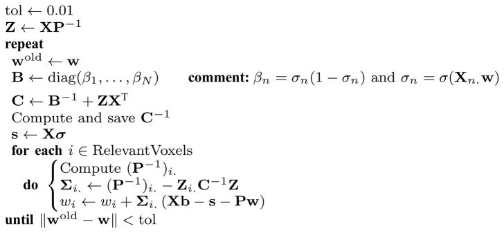
V. Experiments

In order to illustrate the ability of RVoxM to yield informative models that predict well, we here present two experiments using T1-weighted structural magnetic resonance imaging (MRI) scans. The first experiment aims at predicting a subject’s age from a volumetric gray matter segmentation (i.e., a regression scenario), whereas the second one focuses on discriminating Alzheimer’s patients from healthy controls using surface-based cortical thickness measurements (illustrating a classification application).

A. Predicting Age

Both the structure and function of the human brain undergo significant changes over a person’s life-time, and these changes can be detected using neuroimaging [49], [50]. Image-based prediction methods for estimating an individual’s age from a brain MRI scan have attracted recent attention [17], [29], [51] since they provide a novel perspective for studying healthy development and aging patterns, while characterizing pathologic deviations in disease. In the current experiment, we employed the publicly available cross-sectional OASIS dataset [52], which consists of 436 subjects aged 18 to 96. For each subject, 3 or 4 individual T1-weighted MRI scans acquired in single scan sessions were averaged to obtain a single high-quality image. The subjects are all right-handed and include both men and women. 100 of the subjects over the age of 60 have been clinically diagnosed with very mild to moderate Alzheimer’s disease (AD).

We processed all the MRI scans with SPM8¹, using default settings, to obtain spatially aligned gray matter maps for each subject. Briefly, the SPM software performs a simultaneous registration and segmentation of each MRI volume [53], aligning the image non-linearly with a standard template while at the same time computing each voxel’s probability of belonging to different tissue types, such as gray or white matter. The resulting gray matter probability maps are then spatially transferred over to the coordinates of the template and modulated by the Jacobian of the non-linear transformations, yielding the so-called gray matter density maps commonly analyzed in voxel-based morphometry (VBM) studies [1].

Unsmoothed gray matter density values were used as the voxel-level measurements x_i in the present experiment. The average gray matter density volume computed on the training data was thresholded at 50% to obtain a mask of voxels that went into the analysis. On the analyzed data, there were an approximate total of 75k voxels in the mask. We employed a 6-connectivity neighborhood to define the Laplacian matrix.

To assess generalization accuracy and stability, we performed 5-fold cross-validation on the data from the cognitively normal and healthy subjects (N = 336, 43.7 ± 23.8 years, 62.5% female). In each cross-validation session, four fifths of the data were used for training an RVoxM. This model was then applied to the remaining fifth for testing. Each training session took about 100 CPU hours with our Matlab implementation, on a Xeon 5472 3.0GHz CPU.

Figure 2 shows the predicted age versus the real age for each subject. Note that each subject was treated as a test subject in only one of the 5 cross-validation sessions; the figure shows the predictions pooled across the sessions. The correlation between the real vs. the predicted age is 0.94, and the root mean square error (RMSE) is less than 7.9 years. It is interesting to note that the deviation from the best fit line seems to increase for older subjects who are beyond middle-age. This is likely driven by latent pathology, as recent studies have estimated that up to 30% of cognitively normal elderly subjects are actually at the pre-clinical stages of Alzheimer’s disease [54].

Fig. 2.

RVoxM based predicted age versus real age in a cohort of 336 cognitively healthy subjects.

Figure 3 illustrates the “relevance voxels” – those voxels that have non-zero contribution in the final prediction model – across the five training sessions. It can be appreciated that most voxels have a zero contribution (i.e., the model is sparse), and that the relevance voxels occur in clusters, providing clear clues as to what parts of the gray matter are driving the age prediction process. Furthermore, the relevance voxels exhibit an overall consistent pattern across the five training sessions, as can be deduced from the yellow regions in the bottom row of Figure 3, thus providing evidence that these patterns are likely to be associated with the underlying biology and can be interpreted. The relevance patterns include peri-sylvian areas (e.g., Heschl’s gyrus) as well as deep structures (e.g., thalamus), and are in broad agreement with published aging-associated morphology maps (e.g., [55]).

Fig. 3.

Relevance voxels for predicting age, overlaid on the average gray matter density image across all subjects. Top row: The μ^* map (eq. (11) in which the hyper-parameters have been set to their optimized values) averaged across 5 cross-validation sessions. Voxels with zero weight are transparent. Bottom row: The frequency at which a voxel was selected as being relevant (i.e., receiving a non-zero weight in a training session) across the 5 cross-validation sessions.

In addition to RVoxM, we also tested two other methods as benchmarks. The first method, referred to as “RVM”, was specifically proposed recently for estimating age from structural MRI [29]. It uses a principal component analysis (PCA) to achieve a dimensionality-reduced representation of the image data, and subsequently applies a linear RVM algorithm in the resulting feature space. We used the optimal implementation settings that were described in [29] and a public implementation of RVM². The second benchmark (“RVoxM-NoReg”) was an implementation of RVoxM with no spatial regularization, i.e., with the hyper-parameter λ intentionally clamped to zero. A comparison with the latter benchmark gives us an insight into the effect of spatial regularization on the results.

Figure 4 plots the average RMSE for all three algorithms (top), as well as the average difference between the individual-level prediction errors (square of predicted age minus true age) obtained by RVoxM and the other two methods (bottom). Overall, RVoxM yields the best accuracy with a RMSE less than 7.9 years – the difference between RVoxM’s performance and the other two benchmarks is statistically significant (paired t-test, P < 0.05). RVoxM also attains the highest correlation (r-value) between the subjects’ real age and predicted age among all three methods: 0.94 for RVoxM vs. 0.9 and 0.93 for RVM and RVoxM-NoReg, respectively. We note that [29] reported a slightly better correlation value for RVM (r = 0.92), which is probably due to the increased sample size (410 training subjects instead of the 268 training subjects used here).

Fig. 4.

Top: average root mean square error for the three age regression models. Bottom: average difference between subject-level prediction errors, measured as the square of real age minus predicted age. (A) Error of RVM minus error of RVoxM. (B) Error of RVoxM-NoReg minus error of RVoxM. Error bars show the standard error of the mean.

Finally, we also examined the deviation of the predicted “brain age” from the real age particularly in elderly subjects. Recent work on a young cohort attributed such a deviation observed in fMRI data to the nonlinear development trajectory of the brain [17]. Moreover, neuroimaging studies on dementia and Alzheimer’s have suggested that these diseases might accelerate atrophy in the brain [56]. As such, we hypothesized that the mini mental state examination (MMSE) score, a cognitive assessment that predicts dementia, may explain some of the non-linear behavior in the predicted “brain age” of elderly subjects. To test this hypothesis, we used the RVoxM from the first of the 5-fold cross-validation experiment, which was trained on 268 cognitively healthy subjects. We applied this RVoxM model to predict the “brain age” of 100 AD patients and 30 cognitively healthy elderly subjects from the test group (see Figure 5). Note that none of these subjects were used to train the RVoxM and we excluded 33 young healthy subjects, for which we did not have an MMSE score. We then conducted a linear regression analysis, where the predicted age was treated as the outcome variable and real age, MMSE and sex were the independent variables. Both the real age (coefficient: 0.84, P-val < 10⁻²²) and the MMSE score (coefficient: −0.77, P-val< 10⁻⁴) were independently associated with the predicted age, but the subject’s sex was not. This suggests that pathological processes that are reflected as cognitive decline might explain some of the deviation in the predicted brain age.

Fig. 5.

RVoxM based predicted age versus real age in a cohort of 30 cognitively healthy subjects and 100 AD patients.

B. Predicting Alzheimer’s Diagnosis

Here we demonstrate RVoxM as a classifier for discriminating healthy controls from AD patients based on their brain MRI scans. Instead of working with volumetric MRI data, we implemented RVoxM on a 2D surface model of the cerebral cortex, further demonstrating the versatility of the proposed algorithm. We applied RVoxM to the publicly available Alzheimer’s Disease Neuroimaging Initiative (ADNI) dataset³, which consisted of 818 subjects at the time of writing. At recruitment, 229 subjects were categorized as cognitively healthy; 396 subjects as amnestic Mild Cognitive Impairment (MCI) – a transitionary, clinically defined pre-AD stage; and 193 subjects as AD. All subjects were clinically followed up every six months, starting from a baseline clinical assessment. Each follow-up visit typically included a cognitive assessment and a structural MRI scan. In the present experiment, we only analyzed baseline MRI scans. We processed all MRI scans with the FreeSurfer software suite [57], [58], computing subject-specific models of the cortical surface as well as thickness measurements across the entire cortical mantle [4]. Subject-level thickness measurements were then transferred to a common coordinate system, represented as a icosohedron-based triangulation of the sphere, via a surface-based nonlinear registration procedure [59], and analyzed by RVoxM. We utilized the so-called fsaverage6 representation, consisting of approximately 82,000 vertices across the two hemispheres with an inter-vertex distance of approximately 2 mm. We emphasize that we did not smooth these cortical thickness maps for any of our experiments. The matrix L for the spatial regularization was obtained by using the neighborhood structure of the triangulated mesh.

Our analysis used MRI scans from 150 AD patients (75.1 ± 7.4 years, 47% female), and an age and sex-matched control group (N=150; cognitively normal (CN); 76.1 ± 5.8 years; 47% female)⁴. As in the age prediction experiment, we conducted a five-fold cross-validation, where each clinical group was first divided into five subgroups. During each fold, one AD and one CN subgroup were set aside as the test set and the RVoxM classification algorithm was trained on the remaining subjects, which took around 110 CPU hours (Matlab implementation, Xeon 5472 3.0GHz CPU). The obtained classification model was then tested on the corresponding test group. The presented results are combined across all five training/test sessions.

For comparison, we also implemented the following four benchmark algorithms:

1. RVoxM-NoReg: Similar to the regression experiment, we implemented the RVoxM classifier with the spatial regularization intentionally switched off, i.e., with λ = 0.

2. SVM: We also applied a linear support vector machine (SVM) classifier, a demonstrated state-of-the-art AD classification method [39], to the cortical thickness maps. For this purpose, we used the popular SVM implementation provided by the freely available LIBSVM software package [60].

3. SVM-Seg: We applied the same linear SVM implementation to thickness measurements in 70 automatically segmented cortical subregions. In particular, we used FreeSurfer to parcellate the entire cortical mantle based on the underlying sulcal pattern [61], computed a list of average thickness measurements for each of the resulting subregions, and used these as the attribute vector for the SVM.

4. RVM-Seg: Finally, we also applied an implementation of the RVM binary classifier⁵ with a linear kernel to the same thickness measurements of the 70 cortical ROIs used for SVM-Seg.

Figure 6 shows the receiver operating characteristics (ROC) curve for RVoxM and the four benchmark algorithms. The ROC curves were generated by varying a threshold applied to the continuous prediction score that each of the algorithms generates (eq. (26) for RVoxM). For each threshold value, we computed the specificity and sensitivity values on each test group corresponding to each of the five folds. These specificity and sensitivity values were then averaged to obtain the presented ROC curves. Based on the area under the ROC curve (AUC), SVM (93%) and RVoxM (93%) perform the best for discriminating AD patients from healthy controls.

Fig. 6.

The receiver operating characteristics curve for five classifiers discriminating between AD patients and controls. Area under the curve values are listed in parentheses in the legend. See text for a description of the methods.

There is a clear difference between RVoxM and RVoxM-NoReg (AUC: 89%), which once again underscores the significance of incorporating the spatial smoothness term into the model. Although SVM and RVoxM have a similar classification performance, it is worth emphasizing that SVM uses all 82,000 mesh vertices simultaneously to make its predictions, complicating the interpretation of its underlying models.

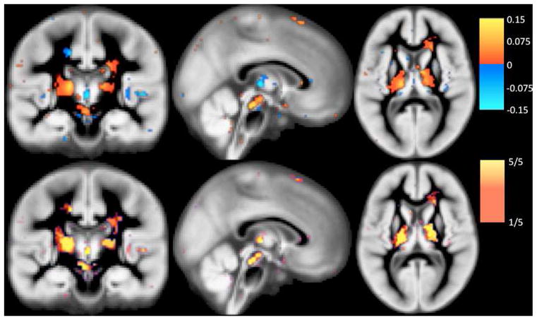
Figure 7 illustrates the RVoxM “relevance vertices” that play a role in discriminating the two clinical groups based on thickness measurements. This figure shows the average μ^* values, where the average was taken across the five cross-validation sessions. Similar to the regression result, one can appreciate that a large number of vertices have a zero contribution (i.e., the model is sparse), and that the relevance vertices appear in spatial clusters. Figure 8 shows the frequency at which each relevance vertex was selected (i.e., had a nonzero contribution) across the five cross-validation sessions. There are certain regions that consistently contribute across the different training sessions (in particular those colored yellow). These vertices include the entorhinal cortex, superior temporal sulcus and posterior cingulate/precuneus, and overlap the so-called default network regions that are known to be targeted in AD [62]. However, there are other regions (mostly in shades of red) that are less consistent and are chosen only in one or two training sessions. We will discuss the possible causes of such model instabilities, as well as ways to mitigate their effect, in section VI.

Fig. 7.

Relevance “voxels” (or more accurately: vertices) for AD vs. control discrimination. The weights for the classification model, μ^* (eq. (24) in which the hyper-parameters have been set to their optimized values), averaged across 5 cross-validation sessions, are illustrated on an inflated cortical representation, overlaid on the folding pattern of the FreeSurfer template subject. Blue regions have a negative contribution (assuming AD is positive) and red regions exhibit a positive weight. Voxels with zero contribution are transparent.

Fig. 8.

The frequency at which each vertex had a non-zero contribution in the final model across the five cross-validation sessions. Transparent voxels never had a non-zero contribution.

We also used the RVoxM model from the first of the 5-fold cross-validation training sessions to compute an “AD score” (eq. (26) for all remaining ADNI subjects, which we subdivided into four groups: (1) cognitively normal, healthy controls, who remained so throughout the study and who were not included in the training data set (N = 109); (2) subjects with MCI who were stable and did not progress to dementia (sMCI, N = 221); (3) subjects who had MCI at baseline but then progressed to AD (pMCI; N = 159); and (4) AD patients (N = 73). Figure 9 plots the average AD score for each of these groups, computed from their baseline MRI scans. We observe that, at baseline, the stable MCI group has an average AD score less than 0.5 and therefore appears more “control-like”, whereas the progressive MCI group has a more “AD-like” average AD score that is greater than 0.5. These results suggest that an RVoxM based classification of someone’s MRI scan might be informative for predicting future clinical decline. To test this hypothesis directly, we conducted a survival analysis with a Cox regression model [63] on all MCI subjects combined (N = 380), where the outcome of interest was time-to-diagnosis. Age, sex, education (years), APOE ε4 allele count, APOE ε3 allele count and the RVoxM-based AD score were entered as independent variables. The only variable that was associated with time-to-diagnosis was the RVoxM-based AD score (coefficient: 0.66, P-val < 10⁻³). This results suggests that a baseline MRI scan contains predictive information about future clinical decline and this information is, to some extent, extracted by the RVoxM AD classifier.

Fig. 9.

Average RVoxM-based AD score for four groups in ADNI. Error bars indicate standard error of the mean.

VI. Discussion and Conclusion

In this paper, we presented the Relevance Voxel Machine (RVoxM), a novel Bayesian model for image-based prediction that is designed to yield intuitive and interpretable results. It allows the predictive influence of individual voxels to vary, and to be more similar in biologically related areas than in completely unrelated ones. Bayesian analysis is then used to select the appropriate form of the model based on annotated training data. As demonstrated in our experiments, RVoxM yields models that are sparse and spatially smooth when spatial proximity is used as a measure of biological connectivity. We believe that such models are easier to interpret than models that use all the image voxels simultaneously, or that base their predictions on a set of isolated voxels scattered throughout the image area. Importantly, our experiments also indicate that RVoxM automatically avoids over-fitting to the training data and produces excellent predictions on test data.

Compared to other prediction models used in medical image analysis, RVoxM offers the following advantages:

• Regularization, feature selection, and biological consistency within a single algorithm;

• Automatic tuning of all parameters, i.e., no free parameters to set manually or via cross-validation; and

• Probabilistic classification predictions, rather than binary decision outcomes.

Although we only applied RVoxM to structural gray matter morphometry in this paper, the method is general and can be extended to handle multiple tissue types at the same time; analyze functional or metabolic imaging modalities; or include non-imaging sources of information such as blood tests, cerebrospinal fluid (CSF) markers, and genetic or demographic data [28]. Furthermore, one can easily incorporate more advanced measures of biological connectivity than the simple spatial smoothness prior used in our experiments. Connectivity information based on symmetry (if the two hemispheres are expected to have similar contributions) or obtained from functional or diffusion imaging can be added by including extra terms “||Γw||²” in eq. (3), with corresponding hyper-parameters that will then be automatically learned from the training data as well.

When discussing the properties of RVoxM, it is useful to consider the training-phase optimization of its hyper-parameters within an ideal Bayesian framework, which would not involve any optimization at all. For the sake of clarity, we will concentrate on the regression case only, although similar arguments apply to the classification case as well. Letting η = (ln α₁, …, ln α_M, ln λ, ln β)^T denote the collection of log-transformed hyper-parameters⁶, and assuming a uniform prior distribution on η: p(η) ∝ 1, the true Bayesian predictive distribution over the target variable t for a new input image x is given by

$$p(t\mid \mathbf{x},\mathbf{X},\mathbf{t})={\int }_{\mathit{\eta }}{\int }_{\mathbf{w}}p(t,\mathbf{w},\mathit{\eta }\mid \mathbf{x},\mathbf{X},\mathbf{t})\text{d}\mathbf{w}\text{d}\mathit{\eta },$$

which involves integrating over both w and η. RVoxM effectively performs the integration over w analytically, while approximating the remaining integral over η, assuming it is dominated by the optimal hyper-parameter value η^* = arg max_ηp(η|X, t):

$$\begin{array}{l}p(t\mid \mathbf{x},\mathbf{X},\mathbf{t})={\int }_{\mathit{\eta }}p(t\mid \mathbf{x},\mathbf{X},\mathbf{t},\mathit{\eta })p(\mathit{\eta }\mid \mathbf{X},\mathbf{t})\text{d}\mathit{\eta }\\ \simeq p(t\mid \mathbf{x},\mathbf{X},\mathbf{t},{\mathit{\eta }}^{\ast }).\end{array}$$ (29)

RVoxM first estimates η^* by maximizing p(η|X, t) ∝ p(t|X, η) (optimization of eq. (5)), and then uses the resulting distribution p(t|x, X, t, η^*) to make predictions (eq. (15)).

The approximation of eq. (29) has the disadvantage that it gives rise to a high-dimensional, non-convex optimization problem, putting RVoxM at risk of local optima and other convergence issues [64]. As demonstrated in [65], these problems can be avoided by approximating the integral over η using Monte Carlo sampling instead: given enough samples from the posterior p(η|X, t), the resulting predictive distribution can be made arbitrarily close to the true one. Although theoretically superior to RVoxM, this approach will only be computationally feasible when a small subset of potentially relevant image voxels are somehow selected a priori [65], limiting its appeal in practical settings.

The ideal Bayesian prediction model that RVoxM approximates also helps explain why RVoxM tends to set many voxel weights to zero values, even though its prior (eq. (4)) may not seem to encourage such solutions. Writing

$$p(t\mid \mathbf{X},\mathbf{t},\mathbf{x})={\int }_{\mathbf{w}}p(t\mid \mathbf{X},\mathbf{t},\mathbf{x},\mathbf{w})p(\mathbf{w}\mid \mathbf{X},\mathbf{t})\text{d}\mathbf{w}$$

reveals that the predictive distribution is obtained by adding contributions of all possible values of w, each weighed by its posterior probability p(w|X, t). Although the integral over w can not easily be approximated to obtain a practically useful algorithm [44], [66], the crucial insight is that the posterior p(w|X, t) ∝ p(t|X, w)p(w) will be high for w’s with many zero entries, because the “true” prior

$$p(\mathbf{w})={\int }_{\mathit{\eta }}p(\mathbf{w}\mid \mathit{\eta })p(\mathit{\eta })\text{d}\mathbf{w},$$ (30)

obtained by integrating out the hyper-parameters, encourages such solutions. Indeed, for the special case where the spatial smoothness hyper-parameter λ is clamped to zero but otherwise p(η) ∝ 1, eq. (30) evaluates to [44]:

$$p(\mathbf{w})\propto \prod _{i}1/\mid w_i\mid ,$$

which is sharply peaked at zero for each voxel and therefore favors sparsity. This “true” prior can be compared to the so-called Laplace prior p(w) ∝ Π_i exp(−|w_i|) often used to obtain sparsity in Bayesian models [67], or – taking the negative log – as the ℓ₁ norm Σ_i |w_i| in the popular “lasso” regularized regression method [68].

RVoxM goes beyond merely inducing sparsity in the models by allowing non-zero values for the hyper-paramer λ, enforcing spatial consistency. This helps remedy the well-known problem with sparsity-only promoting methods that when several variables (i.e., voxels) have similar prediction power, only one tends to be picked with little regard as to which one [69], [70]. In order to avoid such overly sparse models, which hamper biological interpretation, a popular solution in regularized regression is the so-called “elastic net”, which adds a ℓ₂ regularization term to the sparsity-inducing ℓ₁ regularizer of lasso [70]. In Bayesian approaches, proposed remedies include using hyper-parameters that optimize another objective function than the likelihood [69], or assuming voxels belong to a small set of clusters with common regularization [65], [71]. The way RVoxM addresses this issue is by expanding the family of candidate models that can be tried to explain the training data, relying on the fact that relatively simple models – with fewer degrees of freedom – tend to provide better explanations than overly complex ones [38]. By also allowing high values of λ, simple and therefore good models are no longer only those in which just a select few predictive voxels are in the model, but especially those in which neigboring, similarly predictive voxels are in the model together.

Because of the way it seeks sparse but spatially connected solutions, RVoxM is closely related to so-called “structured sparsity”-inducing methods, which aim at selecting problem-relevant groups of variables for inclusion in the model, rather than single variables individually [72]–[76]. In such methods, group-level sparsity is often obtained by variations on the so-called “group lasso”, a generalization of lasso in which the ℓ₂ norm of each group, rather than the amplitude of individual variables, is penalized using the ℓ₁ norm [77], [78]. Perhaps most closely related to RVoxM is the so-called “smooth lasso” method, a variant of the elastic net in which the ℓ₁ norm for sparsity is preserved, but the ℓ₂ norm on the variables themselves is replaced by an ℓ₂ norm on their spatial derivatives [79].

An issue we have not fully addressed in this work is quantifying how repeatable the relevant voxel set is when the RVoxM model is trained on different subjects drawn from the same population. Although the relevant voxel pattern was quite consistent across different training datasets in our regression experiment (see bottom row of Figure 3), there was an appreciable amount of variation in the classification case (see Figure 8). We believe such variations can be further decreased by making more relevant anatomical information available to the RVoxM model – e.g., by including a symmetry regularization term in the prior. The stability of the relevant patterns and the predictions can also be improved by using randomization experiments, in which different models are learned from resampled training data to obtain an average, ensemble prediction model [80], or to select only those voxels that appear frequently across the different models [81], [82]. Instability of informative feature sets has been studied extensively in the literature [83], [84], and can be attributed to three related factors: (1) the limited amount of training data and over-fitting to the quirks of these data, (2) the mismatch between the utilized model and the underlying true discriminative pattern, and (3) the local optima the numerical solver might get trapped in. All three factors apply to the case of RVoxM, and a detailed analysis of these effects will be carried out in future work, using techniques similar to the ones employed in [85]–[87].

One drawback of the presented training algorithm is its computational complexity, which under typical conditions is quadratic in the number of voxels. Our experiments demonstrate that, using standard Matlab code, we can train on a dataset of relatively high-resolution data from hundreds subjects in a matter of days. This computation time, we believe, is acceptable for such datasets that can take years to collect. It is worth emphasizing that a heavy computational burden is incurred only once for a given training dataset and that, after the model has been trained, making predictions on new images is very fast. Since RVoxM automatically tunes all its hyper-parameters within a single training session, there is no need for the repeated cross-validation training runs that are necessary in most other image-based prediction methods and that also take time. Furthermore, more advanced regularization terms can be added to the prior of RVoxM with minimal additional computational cost, whereas the number of training runs required to set the corresponding hyper-parameters using cross-validation would increase exponentially and quickly become impractical.

Although the reported computation times can be reduced significantly by using a non-Matlab based implementation that exploits the parallellization opportunities inherent in Algorithm IV.1; classification problems with more than two classes, as well as higher-resolution and much larger datasets, will still present a serious computational challenge to analyze with RVoxM. The training algorithm we have presented starts with all voxels included in the initial model, and gradually prunes the vast majority of the voxels as the iterations progress. Although this causes the algorithm to gradually speed up, the computational complexity of the first few iterations is still quadratic in the number of voxels. Similar to the dramatically accelerated training procedure for RVM models developed in [88], we are therefore investigating an alternative, “constructive” approach that starts with an empty model and sequentially adds voxels instead, while also modifying the weights of the voxels already in the model. In [88], this was accomplished by deriving an analytical expression for the optimal weight of a voxel, given the current weight of all other voxels; we are currently exploring if a similar approach is also possible for RVoxM.

Appendix A Derivations for the Regression Model

We here derive various partial derivatives of ln p(t|X, α, β, λ) with respect to the hyper-parameters α, β, and λ.

Using the determinant identity

$$\mid {\beta }^{-1}\mathbf{I}+{\mathbf{XP}}^{-1}{\mathbf{X}}^{\text{T}}\mid =\frac{\mid {\beta }^{-1}\mathbf{I}\mid \mid \beta {\mathbf{X}}^{\text{T}}\mathbf{X}+\mathbf{P}\mid }{\mid \mathbf{P}\mid }$$

and Woodbury’s inversion identity

$${({\beta }^{-1}\mathbf{I}+{\mathbf{XP}}^{-1}{\mathbf{X}}^{\text{T}})}^{-1}=\beta \mathbf{I}-\beta \mathbf{X}{(\beta {\mathbf{X}}^{\text{T}}\mathbf{X}+\mathbf{P})}^{-1}{\mathbf{X}}^{\text{T}}\beta ,$$

we can write ln p(t|X, α, β, λ) as:

$$\begin{array}{l}lnp(\mathbf{t}\mid \mathbf{X},\mathit{\alpha },\beta ,\lambda )=-\frac{N}{2}ln(2\pi )-\frac{1}{2}ln\mid \mathbf{C}\mid -\frac{1}{2}{\mathbf{t}}^{\text{T}}{\mathbf{C}}^{-1}\mathbf{t}\\ =-\frac{N}{2}ln(2\pi )+\frac{N}{2}ln\beta -\frac{1}{2}ln\mid {\mathbf{\sum }}^{-1}\mid +\frac{1}{2}ln\mid \mathbf{P}\mid -\frac{1}{2}{\mathbf{t}}^{\text{T}}(\beta \mathbf{I}-\beta \mathbf{X}\mathbf{\sum }{\mathbf{X}}^{\text{T}}\beta )\mathbf{t}.\end{array}$$ (31)

Using Σ⁻¹= βX^TX + diag(α) + λL, we obtain

$$\begin{array}{l}\frac{\partial ln\mid {\mathbf{\sum }}^{-1}\mid }{\partial {\alpha }_i}=\text{trace}\left(\mathbf{\sum }\frac{\partial \text{diag}(\mathit{\alpha })}{\partial {\alpha }_i}\right)\\ ={\mathrm{\sum }}_{ii},\end{array}$$ (32)

and similarly

$$\begin{array}{l}\frac{\partial ln\mid {\mathbf{\sum }}^{-1}\mid }{\partial \beta }=\text{trace}(\mathbf{\sum }{\mathbf{X}}^{\text{T}}\mathbf{X})\\ =\text{trace}(\mathbf{X}\mathbf{\sum }{\mathbf{X}}^{\text{T}})\end{array}$$ (33)

and

$$\frac{\partial ln\mid {\mathbf{\sum }}^{-1}\mid }{\partial \lambda }=\text{trace}(\mathbf{\sum }\mathbf{L}).$$ (34)

Using the same technique on P = diag(α) + λL, we have

$$\frac{\partial ln\mid \mathbf{P}\mid }{\partial {\alpha }_i}={({\mathbf{P}}^{-1})}_{ii}$$ (35)

and

$$\frac{\partial ln\mid \mathbf{P}\mid }{\partial \lambda }=\text{trace}({\mathbf{P}}^{-1}\mathbf{L})$$ (36)

Finally, we have

$$\begin{array}{l}\frac{\partial ({\mathbf{t}}^{\text{T}}\mathbf{X}\mathbf{\sum }{\mathbf{X}}^{\text{T}}\mathbf{t})}{\partial {\alpha }_i}=\frac{\partial \left({\mathbf{t}}^{\text{T}}\mathbf{X}{({\mathbf{\sum }}^{-1})}^{-1}{\mathbf{X}}^{\text{T}}\mathbf{t}\right)}{\partial {\alpha }_i}\\ =-{\mathbf{t}}^{\text{T}}\mathbf{X}\mathbf{\sum }\frac{\partial {\mathbf{\sum }}^{-1}}{\partial {\alpha }_i}\mathbf{\sum }{\mathbf{X}}^{\text{T}}\mathbf{t}\\ =-\frac{1}{\beta }{\mathit{\mu }}^{\text{T}}\frac{\partial \text{diag}(\mathit{\alpha })}{\partial {\alpha }_i}\mathit{\mu }\frac{1}{\beta }\\ =-\frac{{\mu }_i^2}{{\beta }^2},\end{array}$$ (37)

and similarly

$$\frac{\partial ({\mathbf{t}}^{\text{T}}\mathbf{X}\mathbf{\sum }{\mathbf{X}}^{\text{T}}\mathbf{t})}{\partial \beta }=\frac{-1}{{\beta }^2}{\mathit{\mu }}^{\text{T}}{\mathbf{X}}^{\text{T}}\mathbf{X}\mathit{\mu }$$ (38)

and

$$\frac{\partial ({\mathbf{t}}^{\text{T}}\mathbf{X}\mathbf{\sum }{\mathbf{X}}^{\text{T}}\mathbf{t})}{\partial \lambda }=-\frac{1}{{\beta }^2}{\mathit{\mu }}^{\text{T}}\mathbf{L}\mathit{\mu }.$$ (39)

To obtain eq. (7), we take the partial derivative of eq. (31) with respect to α_i and plug in the result of eq. (32), (35), and (37), yielding

$$\frac{\partial lnp(\mathbf{t}\mid \mathbf{X},\mathit{\alpha },\lambda ,\beta )}{\partial {\alpha }_i}=-\frac{1}{2}{\mathrm{\sum }}_{ii}+\frac{1}{2}{({\mathbf{P}}^{-1})}_{ii}-\frac{1}{2}{\mu }_i^2.$$ (40)

Rewriting P⁻¹ using Woodbury’s inversion identity as

$$\begin{array}{l}{\mathbf{P}}^{-1}=\text{diag}(\frac{1}{\mathit{\alpha }})-\text{diag}(\frac{1}{\mathit{\alpha }}){\left(\mathbf{I}+\lambda \mathbf{L}\text{diag}(\frac{1}{\mathit{\alpha }})\right)}^{-1}\lambda \mathbf{L}\text{diag}(\frac{1}{\mathit{\alpha }})\\ =\text{diag}(\frac{1}{\mathit{\alpha }})-\lambda {\mathbf{P}}^{-1}\mathbf{L}\text{diag}(\frac{1}{\mathit{\alpha }})\end{array}$$ (41)

and plugging this result into eq. (40), we finally obtain eq. (7).

Taking the partial derivative of eq. (31) with respect to β and plugging in eq. (33) and (38) yields

$$\frac{\partial lnp(\mathbf{t}\mid \mathbf{X},\mathit{\alpha },\lambda ,\beta )}{\partial \beta }=\frac{N}{2\beta }-\frac{1}{2}\text{trace}(\mathbf{X}\mathbf{\sum }{\mathbf{X}}^{\text{T}})-\frac{1}{2}{\mathbf{t}}^{\text{T}}\mathbf{t}+{\mathbf{t}}^{\text{T}}\mathbf{X}\mathit{\mu }-\frac{1}{2}{\mathit{\mu }}^{\text{T}}{\mathbf{X}}^{\text{T}}\mathbf{X}\mathit{\mu }$$ (42)

which explains eq. (8). Similarly, we obtain eq. (9) by taking the partial derivative of eq. (31) with respect to λ and plugging in eq. (34), (36), and (39).

Appendix B Non-negative properties of the update rules

We here show that the update equations (12) and (13) always yield non-negative values.

For eq. (12), we have:

$$\begin{array}{l}{\alpha }_i^{\text{new}}=\frac{1-{\alpha }_i{\mathbf{\sum }}_{ii}-\lambda {({\mathbf{P}}^{-1}\mathbf{L})}_{ii}}{{\mu }_i^2}\\ =\frac{{\alpha }_i{({\mathbf{P}}^{-1}-\mathbf{\sum })}_{ii}}{{\mu }_i^2}\end{array}$$ (43)

$$\begin{array}{l}=\frac{{\alpha }_i{({\mathbf{P}}^{-1}-{\mathbf{P}}^{-1}+{\mathbf{Z}}^{\text{T}}{\mathbf{C}}^{-1}\mathbf{Z})}_{ii}}{{\mu }_i^2}\\ =\frac{{\alpha }_i}{{\mu }_i^2}{\mathbf{z}}_i^T{\mathbf{C}}^{-1}{\mathbf{z}}_i\ge 0,\end{array}$$ (44)

where we have used eq. (41) to obtain eq. (43), and expanded Σ using eq. (27) to obtain eq. (44). C is the positive semi-definite matrix defined in eq. (6) and z_i is the i’th column of Z = XP⁻¹.

For eq. (13) we have:

$$\begin{array}{l}{\beta }^{\text{new}}=\frac{N-\text{trace}(\beta \mathbf{X}\mathbf{\sum }{\mathbf{X}}^{\text{T}})}{{\left|\right|\mathbf{t}=\mathbf{X}\mathit{\mu }\left|\right|}^2}\\ =\frac{N-\text{trace}(\beta {\mathbf{X}}^{\text{T}}\mathbf{X}\mathbf{\sum })}{{\left|\right|\mathbf{t}-\mathbf{X}\mathit{\mu }\left|\right|}^2}\\ =\frac{N-\text{trace}(({\mathbf{\sum }}^{-1}-\mathbf{P})\mathbf{\sum })}{{\left|\right|\mathbf{t}-\mathbf{X}\mathit{\mu }\left|\right|}^2}\\ =\frac{\text{trace}(\mathbf{P}\mathbf{\sum })}{{\left|\right|\mathbf{t}-\mathbf{X}\mathit{\mu }\left|\right|}^2}\\ =\frac{\text{trace}({\mathbf{S}}^{\text{T}}\mathbf{PS})}{{\left|\right|\mathbf{t}-\mathbf{X}\mathit{\mu }\left|\right|}^2}\\ =\frac{{\sum }_i{\mathbf{s}}_i^{\text{T}}\mathbf{P}{\mathbf{s}}_i}{{\left|\right|\mathbf{t}-\mathbf{X}\mathit{\mu }\left|\right|}^2}\ge 0,\end{array}$$ (45)

where we have used Σ = (P + βX^TX)⁻¹, Σ = SS^T is the Cholesky decomposition of Σ, s_i is the i’th column of S and the inequality is due to P being positive semi-definite.

Appendix C Derivations for the Classification Model

We here explain how we compute the most probable voxel weights in the classification model (eq. (23)) and locally approximate the classification training problem by a regression one (eq. (22)).

For a given set of hyper-parameters {α, λ}, we compute the voxel weights w_MP maximizing the posterior distribution p(w|X, b, α, λ) ∝ p(b|X, w)p(w|α, λ) by using Newton’s method, i.e., by repeatedly performing

$${\mathbf{w}}^{\text{new}}=\mathbf{w}-{\left(\nabla \nabla lnp(\mathbf{w}\mid \mathbf{X},\mathbf{b},\mathit{\alpha },\lambda )\right)}^{-1}\nabla lnp(\mathbf{w}\mid \mathbf{X},\mathbf{b},\mathit{\alpha },\lambda )$$

until convergence, with gradient

$$\nabla lnp(\mathbf{w}\mid \mathbf{X},\mathbf{b},\mathit{\alpha },\lambda )={\mathbf{X}}^{\text{T}}(\mathbf{b}-\mathbf{\sigma })-\mathbf{Pw}$$

and Hessian matrix

$$\nabla \nabla lnp(\mathbf{w}\mid \mathbf{X},\mathbf{b},\mathit{\alpha },\mathit{\lambda })=-({\mathbf{X}}^{\text{T}}\mathbf{BX}+\mathbf{P}),$$

where we have defined σ = (σ₁ …, σ_N )^T, ${\sigma }_n=\sigma ({\mathbf{x}}_n^{\text{T}}\mathbf{w})$, B = diag(β₁, …, β_N ), and β_n = σ_n(1 − σ_n). Since the Hessian is always positive definite, ln p(w|X, b, α, λ) is concave and therefore has a unique maximum [41].

Once the optimum weights w_MP are obtained, we approximate the integral in eq. (21) by replacing the integrand with an unnormalized Gaussian centered around w_MP (Laplace approximation), yielding:

$$lnp(\mathbf{b}\mid \mathbf{X},\mathit{\alpha },\lambda )\simeq ln\left[p(\mathbf{b}\mid \mathbf{X},{\mathbf{w}}_{\text{MP}})p({\mathbf{w}}_{\text{MP}}\mid \mathit{\alpha },\lambda )\sqrt{\frac{{(2\pi )}^M}{\mid \mathbf{H}\mid }}\right]$$ (46)

for the log marginal likelihood, where we have defined

$$\mathbf{H}={-\nabla \nabla lnp(\mathbf{w}\mid \mathbf{X},\mathbf{b},\mathit{\alpha },\lambda )\mid }_{\mathbf{w}={\mathbf{w}}_{\text{MP}}.}$$

Around the most probable voxel weights w̃_MP corresponding to some hyper-parameters {α̃, λ̃} (eq. (23)), we can linearize $\sigma ({\mathbf{x}}_n^{\text{T}}\mathbf{w})$ as follows:

$$\sigma ({\mathbf{x}}_n^{\text{T}}\mathbf{w})\simeq \sigma ({\mathbf{x}}_n^{\text{T}}{\stackrel{\sim }{\mathbf{w}}}_{\text{MP}})+{\stackrel{\sim }{\beta }}_n{\mathbf{x}}_n^{\text{T}}(\mathbf{w}-{\stackrel{\sim }{\mathbf{w}}}_{\text{MP}}),$$

and therefore

$$\mathbf{\sigma }\simeq \mathbf{\sigma }+\stackrel{\sim }{\mathbf{B}}\mathbf{X}(\mathbf{w}-{\stackrel{\sim }{\mathbf{w}}}_{\text{MP}}).$$

As a result, we have that

$$\begin{array}{l}\nabla lnp(\mathbf{b}\mid \mathbf{X},\mathbf{w})={\mathbf{X}}^{\text{T}}(\mathbf{b}-\mathbf{\sigma })\\ \simeq {\mathbf{X}}^{\text{T}}(\mathbf{b}-\stackrel{\sim }{\mathbf{\sigma }}+\stackrel{\sim }{\mathbf{B}}\mathbf{X}{\stackrel{\sim }{\mathbf{w}}}_{\text{MP}}-\stackrel{\sim }{\mathbf{B}}\mathbf{Xw})\\ ={\mathbf{X}}^{\text{T}}\stackrel{\sim }{\mathbf{B}}(\stackrel{\sim }{\mathbf{t}}-\mathbf{Xw})\end{array}$$

and therefore that

$$lnp(\mathbf{b}\mid \mathbf{X},\mathbf{w})\simeq ln\mathcal{N}(\stackrel{\sim }{\mathbf{t}}\mid \mathbf{Xw},{\stackrel{\sim }{\mathbf{B}}}^{-1})+\text{const},$$ (47)

where the constant depends only on w̃_MP. Using this result, we obtain

$$\mathbf{H}\simeq {\mathbf{X}}^{\text{T}}\stackrel{\sim }{\mathbf{B}}\mathbf{X}+\mathbf{P}={\mathbf{\sum }}^{-1},$$ (48)

and because

$${\nabla p(\mathbf{w}\mid \mathbf{X},\mathbf{b},\mathit{\alpha },\lambda |)\mid }_{\mathbf{w}={\mathbf{w}}_{\text{MP}}}=0$$

also that

$${\mathbf{X}}^{\text{T}}\stackrel{\sim }{\mathbf{B}}(\stackrel{\sim }{\mathbf{t}}-\mathbf{X}{\mathbf{w}}_{\text{MP}})-\mathbf{P}{\mathbf{w}}_{\text{MP}}\simeq 0$$

and therefore

$${\mathbf{w}}_{\text{MP}}\simeq \mathbf{\sum }{\mathbf{X}}^{\text{T}}\stackrel{\sim }{\mathbf{B}}\stackrel{\sim }{\mathbf{t}}.$$ (49)

Plugging eq. (47) and (48) into (46), we have that

$$\begin{array}{l}lnp(\mathbf{b}\mid \mathbf{X},\mathit{\alpha },\lambda )\simeq -\frac{N}{2}ln(2\pi )+\frac{1}{2}ln\mid \stackrel{\sim }{\mathbf{B}}\mid -\frac{1}{2}{(\stackrel{\sim }{\mathbf{t}}-\mathbf{Xw})}^{\text{T}}\stackrel{\sim }{\mathbf{B}}(\stackrel{\sim }{\mathbf{t}}-\mathbf{Xw})+\frac{1}{2}ln\mid \mathbf{P}\mid -\frac{1}{2}{\mathbf{w}}_{\text{MP}}^{\text{T}}\mathbf{P}{\mathbf{w}}_{\text{MP}}-\frac{1}{2}ln\mid {\mathbf{\sum }}^{-1}\mid +\text{const}\\ \simeq -\frac{N}{2}ln(2\pi )+\frac{1}{2}ln\mid \stackrel{\sim }{\mathbf{B}}\mid -\frac{1}{2}ln\mid {\mathbf{\sum }}^{-1}\mid +\frac{1}{2}ln\mid \mathbf{P}\mid -\frac{1}{2}{\mathbf{t}}^{\text{T}}(\stackrel{\sim }{\mathbf{B}}-\stackrel{\sim }{\mathbf{B}}\mathbf{X}\mathbf{\sum }{\mathbf{X}}^{\text{T}}\stackrel{\sim }{\mathbf{B}})\mathbf{t}+\text{const},\end{array}$$

where we have used eq. (49) in the last step. Comparing this result to eq. (31) finally yields eq. (22).

References

- 1.Ashburner J, Friston KJ. Voxel-based morphometry–the methods. Neuroimage. 2000;11(6):805–821. doi: 10.1006/nimg.2000.0582. [DOI] [PubMed] [Google Scholar]
- 2.Davatzikos C, Genc A, Xu D, Resnick SM. Voxel-based morphometry using the RAVENS maps: methods and validation using simulated longitudinal atrophy. NeuroImage. 2001;14(6):1361–1369. doi: 10.1006/nimg.2001.0937. [DOI] [PubMed] [Google Scholar]
- 3.Chung MK, Worsley KJ, Paus T, Cherif C, Collins DL, Giedd JN, Rapoport JL, Evans AC. A unified statistical approach to deformation-based morphometry. NeuroImage. 2001;14(3):595–606. doi: 10.1006/nimg.2001.0862. [DOI] [PubMed] [Google Scholar]
- 4.Fischl B, Dale AM. Measuring the thickness of the human cerebral cortex from magnetic resonance images. PNAS. 2000;97(20):11050. doi: 10.1073/pnas.200033797. [DOI] [PMC free article] [PubMed] [Google Scholar]
- 5.Worsley KJ, Friston KJ. Analysis of fMRI time-series revisited-again. Neuroimage. 1995;2(3):173–181. doi: 10.1006/nimg.1995.1023. [DOI] [PubMed] [Google Scholar]
- 6.Haynes JD, Rees G. Decoding mental states from brain activity in humans. Nature Reviews Neuroscience. 2006;7(7):523–534. doi: 10.1038/nrn1931. [DOI] [PubMed] [Google Scholar]
- 7.Mitchell TM, Hutchinson R, Niculescu RS, Pereira F, Wang X, Just M, Newman S. Learning to decode cognitive states from brain images. Machine Learning. 2004;57(1):145–175. [Google Scholar]
- 8.Haxby JV, Gobbini MI, Furey ML, Ishai A, Schouten JL, Pietrini P. Distributed and overlapping representations of faces and objects in ventral temporal cortex. Science. 2001;293(5539):2425. doi: 10.1126/science.1063736. [DOI] [PubMed] [Google Scholar]
- 9.Mourão-Miranda J, Bokde ALW, Born C, Hampel H, Stetter M. Classifying brain states and determining the discriminating activation patterns: support vector machine on functional MRI data. NeuroImage. 2005;28(4):980–995. doi: 10.1016/j.neuroimage.2005.06.070. [DOI] [PubMed] [Google Scholar]
- 10.Norman KA, Polyn SM, Detre GJ, Haxby JV. Beyond mind-reading: multi-voxel pattern analysis of fMRI data. Trends in cognitive sciences. 2006;10(9):424–430. doi: 10.1016/j.tics.2006.07.005. [DOI] [PubMed] [Google Scholar]
- 11.Batmanghelich N, Taskar B, Davatzikos C. IPMI. Springer; 2009. A general and unifying framework for feature construction, in image-based pattern classification; pp. 423–434. [DOI] [PubMed] [Google Scholar]
- 12.Davatzikos C, Fan Y, Wu X, Shen D, Resnick SM. Detection of prodromal Alzheimer’s disease via pattern classification of magnetic resonance imaging. Neurobiology of aging. 2008;29(4):514–523. doi: 10.1016/j.neurobiolaging.2006.11.010. [DOI] [PMC free article] [PubMed] [Google Scholar]
- 13.Fan Y, Shen D, Davatzikos C. Classification of structural images via high-dimensional image warping, robust feature extraction, and svm. Medical Image Computing and Computer-Assisted Intervention–MICCAI 2005. 2005:1–8. doi: 10.1007/11566465_1. [DOI] [PubMed] [Google Scholar]
- 14.Klöppel S, Stonnington CM, Chu C, Draganski B, Scahill RI, Rohrer JD, Fox NC, Jack CR, Ashburner J, Frackowiak RSJ. Automatic classification of MR scans in Alzheimer’s disease. Brain. 2008;131(3):681. doi: 10.1093/brain/awm319. [DOI] [PMC free article] [PubMed] [Google Scholar]
- 15.Liu Y, Teverovskiy L, Carmichael O, Kikinis R, Shenton M, Carter CS, Stenger VA, Davis S, Aizenstein H, Becker JT, et al. Discriminative MR image feature analysis for automatic schizophrenia and Alzheimer’s disease classification. Medical Image Computing and Computer-Assisted Intervention–MICCAI 2004. 2004:393–401. [Google Scholar]
- 16.Pohl K, Sabuncu M. Information Processing in Medical Imaging. Springer; 2009. A unified framework for MR based disease classification; pp. 300–313. [DOI] [PMC free article] [PubMed] [Google Scholar]
- 17.Dosenbach NUF, Nardos B, Cohen AL, Fair DA, Power JD, Church JA, Nelson SM, Wig GS, Vogel AC, Lessov-Schlaggar CN, et al. Prediction of individual brain maturity using fMRI. Science. 2010;329(5997):1358. doi: 10.1126/science.1194144. [DOI] [PMC free article] [PubMed] [Google Scholar]
- 18.Ashburner J, Hutton C, Frackowiak R, Johnsrude I, Price C, Friston K. Identifying global anatomical differences: deformation-based morphometry. Human Brain Mapping. 1998;6(5–6):348–357. doi: 10.1002/(SICI)1097-0193(1998)6:5/6<348::AID-HBM4>3.0.CO;2-P. [DOI] [PMC free article] [PubMed] [Google Scholar]
- 19.Golland P. Discriminative direction for kernel classifiers. Advances in Neural Information Processing Systems. 2002;1:745–752. [Google Scholar]
- 20.Lao Z, Shen D, Xue Z, Karacali B, Resnick SM, Davatzikos C. Morphological classification of brains via high-dimensional shape transformations and machine learning methods. Neuroimage. 2004;21(1):46–57. doi: 10.1016/j.neuroimage.2003.09.027. [DOI] [PubMed] [Google Scholar]
- 21.Golland P, Grimson WEL, Shenton ME, Kikinis R. Detection and analysis of statistical differences in anatomical shape. Medical Image Analysis. 2005;9(1):69–86. doi: 10.1016/j.media.2004.07.003. [DOI] [PMC free article] [PubMed] [Google Scholar]
- 22.Fan Y, Shen D, Gur RC, Gur RE, Davatzikos C. COMPARE: classification of morphological patterns using adaptive regional elements. IEEE Transactions on Medical Imaging. 2007;26(1):93–105. doi: 10.1109/TMI.2006.886812. [DOI] [PubMed] [Google Scholar]
- 23.Yamashita O, Sato M, Yoshioka T, Tong F, Kamitani Y. Sparse estimation automatically selects voxels relevant for the decoding of fMRI activity patterns. NeuroImage. 2008;42:1414–1429. doi: 10.1016/j.neuroimage.2008.05.050. [DOI] [PMC free article] [PubMed] [Google Scholar]
- 24.De Martino F, Valente G, Staeren N, Ashburner J, Goebel R, Formisano E. Combining multivariate voxel selection and support vector machines for mapping and classification of fMRI spatial patterns. NeuroImage. 2008;43:44–58. doi: 10.1016/j.neuroimage.2008.06.037. [DOI] [PubMed] [Google Scholar]
- 25.Janousova E, Vounou M, Wolz R, Gray K, Rueckert D, Montana1 G. Fast brain-wide search of highly discriminative regions in medical images: an application to Alzheimer’s disease. Proceedings of Medical Image Understanding and Analysis 2011. 2011:17–21. [Google Scholar]
- 26.Magnin B, Mesrob L, Kinkingnéhun S, Pélégrini-Issac M, Colliot O, Sarazin M, Dubois B, Lehéricy S, Benali H. Support vector machine-based classification of Alzheimer’s disease from whole-brain anatomical MRI. Neuroradiology. 2009;51(2):73–83. doi: 10.1007/s00234-008-0463-x. [DOI] [PubMed] [Google Scholar]
- 27.Desikan RS, Cabral HJ, Hess CP, Dillon WP, Glastonbury CM, Weiner MW, Schmansky NJ, Greve DN, Salat DH, Buckner RL, Fischl B. Automated MRI measures identify individuals with mild cognitive impairment and Alzheimer’s disease. Brain. 2009;132:2048–2057. doi: 10.1093/brain/awp123. [DOI] [PMC free article] [PubMed] [Google Scholar]
- 28.Vemuri P, Gunter JL, Senjem ML, Whitwell JL, Kantarci K, Knopman DS, Boeve BF, Petersen RC, Jack CR., Jr Alzheimer’s disease diagnosis in individual subjects using structural MR images: validation studies. Neuroimage. 2008;39(3):1186–1197. doi: 10.1016/j.neuroimage.2007.09.073. [DOI] [PMC free article] [PubMed] [Google Scholar]
- 29.Franke K, Ziegler G, Kloppel S, Gaser C. Estimating the age of healthy subjects from T1-weighted MRI scans using kernel methods: Exploring the influence of various parameters. NeuroImage. 2010;50(3):883–892. doi: 10.1016/j.neuroimage.2010.01.005. [DOI] [PubMed] [Google Scholar]
- 30.Liang L, Cherkassky V, Rottenberg DA. Spatial SVM for feature selection and fMRI activation detection. Neural Networks, 2006. IJCNN’06. International Joint Conference on; pp. 1463–1469. IEEE, 2006. [Google Scholar]
- 31.Fung G, Stoeckel J. SVM feature selection for classification of SPECT images of Alzheimer’s disease using spatial information. Knowledge and Information Systems. 2007;11(2):243–258. [Google Scholar]
- 32.Xiang Z, Xi Y, Hasson U, Ramadge P. Boosting with spatial regularization. Advances in Neural Information Processing Systems. 2009;22:2107–2115. [Google Scholar]
- 33.Cuingnet R, Chupin M, Benali H, Colliot O. Spatial and anatomical regularization of SVM for brain image analysis. Advances in Neural Information Processing Systems. 2010;23:460–468. [Google Scholar]
- 34.Cuingnet R, Rosso C, Chupin M, Lehricy S, Dormont D, Benali H, Samson Y, Colliot O. Spatial regularization of SVM for the detection of diffusion alterations associated with stroke outcome. Medical Image Analysis. 2011;15:729–737. doi: 10.1016/j.media.2011.05.007. [DOI] [PubMed] [Google Scholar]
- 35.Michel V, Gramfort A, Varoquaux G, Eger E, Thirion B. Total variation regularization for fMRI-based prediction of behaviour. Medical Imaging, IEEE Transactions on. 2011;30(7):1328–1340. doi: 10.1109/TMI.2011.2113378. [DOI] [PMC free article] [PubMed] [Google Scholar]
- 36.Batmanghelich N, Taskar B, Davatzikos C. Generative-discriminative basis learning for medical imaging. IEEE Transactions on Medical Imaging. 2012;31(1):51–69. doi: 10.1109/TMI.2011.2162961. [DOI] [PMC free article] [PubMed] [Google Scholar]
- 37.van Gerven MAJ, Cseke B, de Lange FP, Heskes T. Efficient Bayesian multivariate fMRI analysis using a sparsifying spatio-temporal prior. NeuroImage. 2010;50:150–161. doi: 10.1016/j.neuroimage.2009.11.064. [DOI] [PubMed] [Google Scholar]
- 38.MacKay D. Information Theory, Inference, and Learning Algorithms. Cambridge University Press; 2003. [Google Scholar]
- 39.Cuingnet R, Gerardin E, Tessieras J, Auzias G, Lehéricy S, Habert MO, Chupin M, Benali H, Colliot O. Automatic classification of patients with Alzheimer’s disease from structural MRI: A comparison of ten methods using the ADNI database. NeuroImage. 2011;56(2):766–781. doi: 10.1016/j.neuroimage.2010.06.013. [DOI] [PubMed] [Google Scholar]
- 40.Cortes C, Vapnik V. Support-vector networks. Machine Learning. 1995;20(3):273–297. [Google Scholar]
- 41.Bishop CM. Pattern Recognition and Machine Learning. Springer; 2006. [Google Scholar]
- 42.Sabuncu MR, Van Leemput K. The Relevance Voxel Machine (RVoxM): A Bayesian method for image-based prediction. Lecture Notes in Computer Science. 2011;6893:99–106. doi: 10.1007/978-3-642-23626-6_13. Proceedings of MICCAI2011. [DOI] [PMC free article] [PubMed] [Google Scholar]
- 43.Neal RM. Bayesian Learning for Neural Networks. Springer-Verlag; 1996. Number 118 in Lecture Notes in Statistics. [Google Scholar]
- 44.Tipping ME. Sparse Bayesian learning and the relevance vector machine. Journal of Machine Learning Research. 2001;1:211–244. [Google Scholar]
- 45.MacKay DJC. PhD thesis. California Institute of Technology; 1992. Bayesian Methods for Adaptive Models. [Google Scholar]
- 46.Berger J. Statistical Decision Theory and Bayesian Analysis. 2. Springer; 1985. [Google Scholar]
- 47.Harville DA. Maximum likelihood approaches to variance component estimation and to related problems. Journal of the American Statistical Association. 1977:320–338. [Google Scholar]
- 48.Woodbury MA. Inverting modified matrices. Memorandum report. 1950;42:106. [Google Scholar]
- 49.D’Esposito M, Zarahn E, Aguirre GK, Rypma B. The effect of normal aging on the coupling of neural activity to the bold hemodynamic response. Neuroimage. 1999;10(1):6–14. doi: 10.1006/nimg.1999.0444. [DOI] [PubMed] [Google Scholar]
- 50.Salat DH, Buckner RL, Snyder AZ, Greve DN, Desikan RSR, Busa E, Morris JC, Dale AM, Fischl B. Thinning of the cerebral cortex in aging. Cerebral Cortex. 2004;14(7):721. doi: 10.1093/cercor/bhh032. [DOI] [PubMed] [Google Scholar]
- 51.Ashburner J. A fast diffeomorphic image registration algorithm. Neuroimage. 2007;38(1):95–113. doi: 10.1016/j.neuroimage.2007.07.007. [DOI] [PubMed] [Google Scholar]
- 52.Marcus DS, Wang TH, Parker J, Csernansky JG, Morris JC, Buckner RL. Open access series of imaging studies (OASIS): cross-sectional MRI data in young, middle aged, nondemented, and demented older adults. Journal of Cognitive Neuroscience. 2007;19(9):1498–1507. doi: 10.1162/jocn.2007.19.9.1498. [DOI] [PubMed] [Google Scholar]
- 53.Ashburner J, Friston KJ. Unified segmentation. Neuroimage. 2005;26(3):839–851. doi: 10.1016/j.neuroimage.2005.02.018. [DOI] [PubMed] [Google Scholar]
- 54.Sperling RA, Aisen PS, Beckett LA, Bennett DA, Craft S, Fagan AM, Iwatsubo T, Jack CR, Kaye J, Montine TJ, et al. Toward defining the preclinical stages of Alzheimer’s disease: Recommendations from the National Institute on Aging and the Alzheimer’s Association workgroup. Alzheimer’s and Dementia. 2011 doi: 10.1016/j.jalz.2011.03.003. [DOI] [PMC free article] [PubMed] [Google Scholar]
- 55.Good CD, Johnsrude IS, Ashburner J, Henson RNA, Friston KJ, Frackowiak RSJ. A voxel-based morphometric study of ageing in 465 normal adult human brains. Neuroimage. 2001;14(1):21–36. doi: 10.1006/nimg.2001.0786. [DOI] [PubMed] [Google Scholar]
- 56.Jobst KA, Smith AD, Szatmari M, Esiri MM, Jaskowski A, Hindley N, McDonald B, Molyneux AJ. Rapidly progressing atrophy of medial temporal lobe in Alzheimer’s disease. The Lancet. 1994;343(8901):829–830. doi: 10.1016/s0140-6736(94)92028-1. [DOI] [PubMed] [Google Scholar]
- 57.Dale AM, Fischl B, Sereno MI. Cortical surface-based analysis I: Segmentation and surface reconstruction. Neuroimage. 1999;9(2):179–194. doi: 10.1006/nimg.1998.0395. [DOI] [PubMed] [Google Scholar]
- 58.Fischl B, Sereno MI, Dale AM. Cortical surface-based analysis II: Inflation, flattening, and a surface-based coordinate system. Neuroimage. 1999;9(2):195–207. doi: 10.1006/nimg.1998.0396. [DOI] [PubMed] [Google Scholar]
- 59.Fischl B, Sereno MI, Tootell RBH, Dale AM. High-resolution intersubject averaging and a coordinate system for the cortical surface. Human Brain Mapping. 1999;8(4):272–284. doi: 10.1002/(SICI)1097-0193(1999)8:4<272::AID-HBM10>3.0.CO;2-4. [DOI] [PMC free article] [PubMed] [Google Scholar]
- 60.Chang Chih-Chung, Lin Chih-Jen. LIBSVM: A library for support vector machines. ACM Transactions on Intelligent Systems and Technology. 2011;2:27:1–27. [Google Scholar]
- 61.Desikan RS, Ségonne F, Fischl B, Quinn BT, Dickerson BC, Blacker D, Buckner RL, Dale AM, Maguire RP, Hyman BT, et al. An automated labeling system for subdividing the human cerebral cortex on MRI scans into gyral based regions of interest. Neuroimage. 2006;31(3):968–980. doi: 10.1016/j.neuroimage.2006.01.021. [DOI] [PubMed] [Google Scholar]
- 62.Buckner RL, Snyder AZ, Shannon BJ, LaRossa G, Sachs R, Fotenos AF, Sheline YI, Klunk WE, Mathis CA, Morris JC, et al. Molecular, structural, and functional characterization of Alzheimer’s disease: evidence for a relationship between default activity, amyloid, and memory. The Journal of Neuroscience. 2005;25(34):7709. doi: 10.1523/JNEUROSCI.2177-05.2005. [DOI] [PMC free article] [PubMed] [Google Scholar]
- 63.Cox DR. Regression models and life-tables. Journal of the Royal Statistical Society. Series B (Methodological) 1972:187–220. [Google Scholar]
- 64.Wipf D, Nagarajan S. A new view of automatic relevance determination. In: Platt JC, Koller D, Singer Y, Roweis S, editors. Advances in Neural Information Processing Systems. Vol. 20. MIT Press; Cambridge, MA: 2008. pp. 1625–1632. [Google Scholar]
- 65.Michel V, Eger E, Keribin C, Thirion B. Multiclass sparse Bayesian regression for fMRI-based prediction. Journal of Biomedical Imaging. 2011 Jan;:2:1–2:13. doi: 10.1155/2011/350838. [DOI] [PMC free article] [PubMed] [Google Scholar]
- 66.MacKay DJC. Comparison of approximate methods for handling hyperparameters. Neural Computation. 1999;11(5):1035–1068. [Google Scholar]
- 67.Williams PM. Bayesian regularization and pruning using a Laplace prior. Neural Computation. 1995;7(1):117–143. [Google Scholar]
- 68.Tibshirani R. Regression shrinkage and selection via the lasso. Journal of the Royal Statistical Society. Series B (Methodological) 1996:267–288. [Google Scholar]
- 69.Qi Y, Minka TP, Picard RW, Ghahramani Z. Predictive automatic relevance determination by expectation propagation. Proceedings of the 21st International Conference on Machine Learning. 2004:671–678. [Google Scholar]
- 70.Zou H, Hastie T. Regularization and variable selection via the elastic net. Journal of the Royal Statistical Society: Series B. 2005;67(2):301–320. [Google Scholar]
- 71.Friston K, Chu C, Mourao-Miranda J, Hulme O, Rees G, Penny W, Ashburner J. Bayesian decoding of brain images. NeuroImage. 2008;39:181–205. doi: 10.1016/j.neuroimage.2007.08.013. [DOI] [PubMed] [Google Scholar]
- 72.Bach F. Exploring large feature spaces with hierarchical multiple kernel learning. Advances in Neural Information Processing Systems. 2008:105–112. [Google Scholar]
- 73.Zhao BP, Rocha G, Yu B. The composite absolute penalties family for grouped and hierarchical variable selection. The Annals of Statistics. 2009;37:3468–3497. [Google Scholar]
- 74.Huang J, Zhang T, Metaxas D. Learning with structured sparsity. Journal of Machine Learning Research. 2011;12:3371–3412. [Google Scholar]
- 75.Jenatton R, Audibert J-Y, Bach F. Structured variable selection with sparsity-inducing norms. Journal of Machine Learning Research. 2011;12:2777–2824. [Google Scholar]
- 76.Jenatton R, Gramfort A, Michel V, Obozinski G, Bach F, Thirion B. Multi-scale mining of fMRI data with hierarchical structured sparsity. IEEE International Workshop on Pattern Recognition in NeuroImaging. 2011 [Google Scholar]
- 77.Yuan M, Lin Y. Model selection and estimation in regression with grouped variables. Journal of the Royal Statistical Society: Series B. 2006;68(1):49–67. [Google Scholar]
- 78.Bach FR. Consistency of the group lasso and multiple kernel learning. Journal of Machine Learning Research. 2008;9:1179–1225. [Google Scholar]
- 79.Hebiri M, Van De Geer S. The smooth-lasso and other l1 + l2-penalized methods. ArXiv. 2010:1003. [Google Scholar]
- 80.Wang Y, Fan Y, Bhatt P, Davatzikos C. High-dimensional pattern regression using machine learning: From medical images to continuous clinical variables. NeuroImage. 2010;50:1519–1535. doi: 10.1016/j.neuroimage.2009.12.092. [DOI] [PMC free article] [PubMed] [Google Scholar]
- 81.Bunea F, She Y, Ombao H, Gongvatana A, Devlin K, Cohen R. Penalized least squares regression methods and applications to neuroimaging. NeuroImage. 2011;55:1519–1527. doi: 10.1016/j.neuroimage.2010.12.028. [DOI] [PMC free article] [PubMed] [Google Scholar]
- 82.Varoquaux G, Gramfort A, Thirion B. Small-sample brain mapping: sparse recovery on spatially correlated designs with randomization and clustering. Proceedings of the 29th International Conference on Machine Learning. 2012 [Google Scholar]
- 83.Saeys Y, Inza I, Larrañaga P. A review of feature selection techniques in bioinformatics. Bioinformatics. 2007;23(19):2507. doi: 10.1093/bioinformatics/btm344. [DOI] [PubMed] [Google Scholar]
- 84.Hua J, Tembe WD, Dougherty ER. Performance of feature-selection methods in the classification of high-dimension data. Pattern Recognition. 2009;42(3):409–424. [Google Scholar]
- 85.Himberg J, Hyvärinen A. Icasso: software for investigating the reliability of ICA estimates by clustering and visualization. Neural Networks for Signal Processing, 2003. NNSP’03. 2003 IEEE 13th Workshop on; IEEE. 2003. pp. 259–268. [Google Scholar]
- 86.Saeys Y, Abeel T, Van de Peer Y. Robust feature selection using ensemble feature selection techniques. Machine Learning and Knowledge Discovery in Databases. 2008:313–325. [Google Scholar]
- 87.Plant C, Teipel SJ, Oswald A, Böhm C, Meindl T, Mourao-Miranda J, Bokde AW, Hampel H, Ewers M. Automated detection of brain atrophy patterns based on MRI for the prediction of Alzheimer’s disease. Neuroimage. 2010;50(1):162–174. doi: 10.1016/j.neuroimage.2009.11.046. [DOI] [PMC free article] [PubMed] [Google Scholar]
- 88.Tipping ME, Faul AC. Fast marginal likelihood maximisation for sparse Bayesian models. Proceedings of the Ninth International Workshop on Artificial Intelligence and Statistics. 2003 [Google Scholar]